The Euler Number of Bloch States Manifold and the Quantum Phases in Gapped Fermionic Systems

Abstract

We propose a topological Euler number to characterize nontrivial topological phases of gapped fermionic systems, which originates from the Gauss-Bonnet theorem on the Riemannian structure of Bloch states established by the real part of the quantum geometric tensor in momentum space. Meanwhile, the imaginary part of the geometric tensor corresponds to the Berry curvature which leads to the Chern number characterization. We discuss the topological numbers induced by the geometric tensor analytically in a general two-band model. As an example, we show that the zero-temperature phase diagram of a transverse field XY spin chain can be distinguished by the Euler characteristic number of the Bloch states manifold in a (1+1)-dimensional Bloch momentum space.

I Introduction

Since the discovery of the Berry phase Berry ; Simon contained in the quantum state with cyclic adiabatic evolutions and the topological Chern number interpretation for the adiabatic pumping Thouless ; Niu and the quantized Hall conductance Laughlin ; TKNN ; Niu1984 , the geometric and topological properties have been playing increasingly important roles in quantum physics. Recently, new topological phases described by the $Z_{2}$ numbers have been found in quantum spin Hall effect and in topological insulators Kane ; Fu ; Hasan ; Qi . A significant question is whether there exists other quantum numbers to characterize the topological phases. In this paper, we introduce a new topological quantum number–Euler number to characterize the topological phase of a gapped fermionic ground state, which is based on the Gauss-Bonnet theorem on the Riemannian structure established by the real part of the quantum geometric tensor Provost ; Berry1989 in momentum space.

As a Hermitian metric induced on the quantum states manifold, the quantum geometric tensor originates from defining a local $U(1)$ gauge invariant quantum distance between two states in a parameterized Hilbert space. This effort results in a Riemannian structure of the quantum states manifold, and the corresponding Riemannian metric is given by the real part of the geometric tensor. Remarkably, its imaginary part, canceled out in the quantum distance, was later found to be just the Berry curvature up to a constant coefficient.

The geometric tensor has recently drawn a lot of attention in characterizing the novel collective behaviors of quantum many-body systems in low temperature Resta ; Haldane ; Ma ; Ryu ; Rezakhani . As a more general covariant tensor than the Berry curvature on the Hilbert space geometry, the quantum geometric tensor defined on the ground-state manifold is naturally expected to shed some light on the understanding of quantum phase transitions in many-body systems Sachdev . Indeed, recent studies Zanardi ; Venuti ; Gu2010 have shown that the ground state geometric tensor can provide a unified approach of the fidelity susceptibility Gu2007 and the Berry curvature to demonstrate the singularity and scaling behaviors exhibited in the vicinity of quantum critical point Pachos ; Hamma ; Zhu ; Ma2009 .

On the other hand, the properties of the ground state, i.e., some physical response function, can be insensitive to local perturbations and the system can undergo a topological phase transition Wen , which is beyond the Landau’s second order phase transitions paradigm with the pattern of symmetry breaking and local order parameters. One of the best known examples is the integer quantum Hall effect, where the Hall conductivity is expressed as the first Chern number in the units of $e^{2}/h$. To our knowledge, the previous studies on the ground state geometric tensor are trapped in the local properties, i.e., the fidelity susceptibility and the partial derivatives of Berry phase, and then only the phase boundaries can be witnessed by this approach Abasto ; Yang ; Hamma2008 ; Garnerone . Some works have show that the ground state Berry phases protected by some symmetry can been used as local order parameters to study various topological phases Hatsugai ; Fufu . The $Z_{2}$ number characterization as a quantized Berry phase of Bloch states for spin chain systems has been proposed in our recent work (see Ref.Ma2012 ).

In this work, we introduce a topological Euler number, based on a quantum geometric tensor defined in the Bloch states manifold, to characterize quantum phases of a gapped fermionic ground state. We discuss this approach analytically in a general two-band model. As an example, we show that there exists a topological quantum phase transition in a transverse field XY spin-1/2 chain in (1+1)-dimensional momentum space. We show that the phase diagram can be distinguished by the topological Euler characteristic number, meanwhile, a nontrivial $Z_{2}$ number is also obtained by the integral of the Berry curvature as the imaginary part of the geometric tensor over half of the Brillouin zone, which is converted from the first Chern number for the time-reversal invariant Bloch Hamiltonian.

II Topological Euler number in momentum space

To begin with, we introduce the notion of quantum geometric tensor in Bloch momentum space, which can be derived from a gauge invariant distance between two Bloch states on the $U(1)$ line bundle induced by the quantum adiabatic evolution of the Bloch state $\left|{u}_{n}{\left(k\right)}\right\rangle$ of the $n$-th filled band. The quantum distance between two states $\left|{u}_{n}{\left(k{+\delta k}\right)}\right\rangle$ and $\left|{u}_{n}{\left(k\right)}\right\rangle$ is given by $dS^{2}=\sum_{\mu,\upsilon}\langle{{{\partial_{\mu}u}}}_{n}{{{\left(k\right)dk^{\mu}}}\left|{{{\partial_{\upsilon}u}}}_{n}{{{\left(k\right)dk^{\upsilon}}}}\right\rangle}$, where $\mu,\nu$ denote the components $k^{\mu}$ and $k^{\nu}$, respectively. The term $\left|{\partial_{\mu}u}_{n}\left(k\right)\right\rangle$ can be decomposed as $\left|{\partial_{\mu}u}_{n}{\left(k\right)}\right\rangle=\left|{D_{\mu}u}_{n}{\left(k\right)}\right\rangle{+}\left[\bm{1}-\mathcal{P}(k)\right]{{\left|{\partial_{\mu}u}_{n}{\left(k\right)}\right\rangle}}$, where $\mathcal{P}_{n}(k)=\left|{u}_{n}{\left(k\right)}\right\rangle\left\langle{u}_{n}{\left(k\right)}\right|$ is the projection operator and $\left|{D_{\mu}u\left(k\right)}\right\rangle=\mathcal{P}_{n}(k)\left|{\partial_{\mu}u}_{n}{\left(k\right)}\right\rangle$ is the covariant derivative of $\left|{u}_{n}{\left(k\right)}\right\rangle$ on the line bundle. Under the condition of the quantum adiabatic evolution, the evolution of $\left|{u}_{n}{\left(k\right)}\right\rangle$ to $\left|{u}_{n}{\left(k+\delta k\right)}\right\rangle$ will undergo a parallel transport, then we have $\left|{D_{\mu}u}_{n}{\left(k\right)}\right\rangle=0$. Finally, we can obtain $dS^{2}=\sum_{\mu,\upsilon}\langle{\partial_{\mu}u}_{n}{\left(k\right)}|\left[\bm{1-}\mathcal{P}_{n}(k)\right]\left|{\partial_{{\nu}}u}_{n}{\left(k\right)}\right\rangle{{dk^{\mu}dk^{\upsilon}}}$. The quantum geometric tensor is given by

$$Q_{\mu{\nu}}^{n}=\langle{\partial_{\mu}u}_{n}{\left(k\right)}|\left[\bm{1-}\mathcal{P}_{n}(k)\right]\left|{\partial_{{\nu}}u}_{n}{\left(k\right)}\right\rangle.$$ (1)

The geometric tensor can be rewritten as $Q_{\mu{\nu}}^{n}=\mathcal{G}_{\mu{\nu}}^{n}-i\mathcal{F}_{\mu{\nu}}^{n}/2$, where $\mathcal{G}_{\mu{\nu}}^{n}=$Re$Q_{\mu{\nu}}^{n}\$can be verified as a Riemannian metric, or called the Fubini-Study metric, which establishes a Riemannian manifold of the Bloch states, and then the quantum distance can be written as $dS^{2}=\sum_{\mu,\upsilon}$Re$Q_{\mu{\nu}}^{n}{{dk^{\mu}dk^{\upsilon}}}$. The term $\mathcal{F}_{\mu{\nu}}^{n}=-2$Im$Q_{\mu{\nu}}^{n}$ is canceled out in the summation of the distance due to its antisymmetry, but can associate to a $2$-form $\mathcal{F}^{n}=\sum_{\mu,\upsilon}\mathcal{F}_{\mu{\nu}}^{n}{dk^{\mu}\wedge dk^{\nu}}$, which is nothing but the Berry curvature. The geometric tensor is also a local response function of the Bloch state, we find that the $\mathcal{G}_{\mu{\nu}}^{n}$ can be associated to a distance response as $\lim_{{\Delta k}\rightarrow 0}\left({\Delta}S/{\Delta}k\right)^{2}=\sum_{\mu,\upsilon}\mathcal{G}_{\mu{\nu}}^{n}{\partial}_{k}k{{}^{\mu}}\otimes{\partial}_{k}k^{{\nu}}$ which is just the concept of fidelity susceptibility, and $\mathcal{F}_{\mu{\nu}}^{n}$ can be associated to a phase response function as $\lim_{\sigma\rightarrow 0}\left(\left|{u}_{n}(k)\right\rangle_{\text{Final}}-\left|{u}_{n}(k)\right\rangle_{\text{Initial}}\right)\left|{u}_{n}(k)\right\rangle_{\text{Initial}}^{-1}\sigma^{-1}=\sum_{\mu,\upsilon}\mathcal{F}_{\mu{\nu}}^{n}{\partial}_{k}{k^{\mu}\wedge\partial_{k}{k}}^{{\nu}}$, where $\sigma$ is the area element enclosed by a cyclic path in the momentum space.

Now we consider the topological properties of the geometric tensor in momentum space. Note that the Brillouin zone has the topology of torus if we take the periodic gauge $\left|{u}_{n}{\left(k\right)}\right\rangle=e^{iG\cdot r}\left|{u}_{n}{\left(k+G\right)}\right\rangle$, and then the ground state satisfies $\left|{\Psi\left(k\right)}\right\rangle=\left|{\Psi\left(k+G\right)}\right\rangle$, where $G$ is the reciprocal lattice vector. Without loss of generality, we consider a gapped fermionic Hamiltonian in 2D momentum space, where the unique Bloch state $\left|{u}_{n}{\left(k\right)}\right\rangle$ forms a $U\left(1\right)$ line bundle on a torus $T^{2}$ formed by the 2D Brillouin zone. The corresponding Berry curvature $\mathcal{F}_{\mu{\nu}}^{n}$ for the Bloch state $\left|{u}_{n}{\left(k\right)}\right\rangle$ is given by $\mathcal{F}_{\mu{\nu}}^{n}=-2$Im$\langle{\partial_{\mu}u}_{n}{\left(k\right)}|\left[\bm{1-}\left|{u}_{n}{\left(k\right)}\right\rangle\left\langle{u}_{n}{\left(k\right)}\right|\right]\left|{\partial_{{\nu}}u}_{n}{\left(k\right)}\right\rangle$. The topological invariant on the $U\left(1\right)$ line bundle of all occupied bands is the first Chern number

$$Ch_{1}=\frac{1}{2\pi}\sum_{n}\iint_{\text{Bz}}\mathcal{F}_{\mu{\nu}}^{n}d{k}^{\mu}d{k}^{{\nu}}.$$ (2)

What is more interesting is that there exists another topological invariant —the Euler characteristic number, which originates from the Gauss-Bonnet theorem on the 2D closed manifold established by the Riemannian metric $\mathcal{G}_{\mu{\nu}}^{n}$ for the Bloch state $\left|{u}_{n}{\left(k\right)}\right\rangle$. The theorem states that the number $\chi\left(\mathcal{M}^{2}\right):=\frac{1}{2\pi}\int_{\mathcal{M}^{2}}\mathcal{K}dA$ is a topological invariant named Euler characteristic number and equals to $2\left(1-g\right)$ with genus $g$ for a closed smooth manifold, where $\mathcal{K}$ is the Gauss curvature and $dA$ is the element of area of the surface. In two dimensions, the Euler number of all occupied bands can be calculated using the metric $\mathcal{G}_{\mu{\nu}}^{n}$ as follows

$$\chi=\frac{1}{4\pi}\sum_{n}\iint_{\text{Bz}}\mathcal{R}^{n}\sqrt{\det\left(\mathcal{G}_{\mu{\nu}}^{n}\right)}d{k}^{\mu}d{k}^{{\nu}},$$ (3)

where the $\mathcal{R}^{n}$ is the Ricci scalar curvature associate to the Bloch state $\left|{u}_{n}{\left(k\right)}\right\rangle$ and here the metric $\mathcal{G}_{\mu{\nu}}^{n}=$Re$\langle{\partial_{\mu}u}_{n}{\left(k\right)}|\left[\bm{1-}\left|{u}_{n}{\left(k\right)}\right\rangle\left\langle{u}_{n}{\left(k\right)}\right|\right]\left|{\partial_{{\nu}}u}_{n}{\left(k\right)}\right\rangle$. The Ricci scalar curvature $\mathcal{R}$ can be calculated by the following standard steps: $\mathcal{R}=\mathcal{G}^{ab}R_{ab}$, and $R_{ab}=R_{acb}^{c}$, where the Riemannian curvature tensor $R_{abc}^{d}=\partial_{b}\Gamma_{ac}^{d}-\partial_{a}\Gamma_{bc}^{d}+\Gamma_{ac}^{e}\Gamma_{be}^{d}-\Gamma_{bc}^{e}\Gamma_{ae}^{d}$, and the Levi-Cività connection $\Gamma_{bc}^{a}$ can be calculated by $\Gamma_{bc}^{a}=\frac{1}{2}\mathcal{G}^{ad}\left({\partial}_{b}\mathcal{G}_{dc}+{\partial}_{c}\mathcal{G}_{bd}-{\partial}_{d}\mathcal{G}_{cb}\right)$.

III Analytical results in two-band model

Here let us consider a 1D translational invariant fermionic system with two bands separated by a finite gap. The Hamiltonian can be written as $H=\sum_{l,l^{\prime}\in N}^{\text{PBC}}\Psi_{l,l^{\prime}}^{\dagger}\mathcal{H}_{l,l^{\prime}}\Psi_{l,l^{\prime}}$, where $\Psi_{l,l^{\prime}}^{\dagger}=\left(c_{l}^{\dagger},c_{l^{\prime}}\right)$ denotes a pair of fermionic creation and annihilation operators on the sites $l$ and $l^{\prime}$, $\mathcal{H}_{l,l^{\prime}}$ is a $2\times 2$ Hermitian matrix, and the periodic boundary condition (PBC) has been imposed. In spite of its simplicity, this model has a wide range of applications, such as the Bogoliubov-de Gennes Hamiltonian in superconductivity and graphite systems.

In order to obtain an appropriate definition of geometric tensor to describe the ground state of the system in a 2D manifold, we can perform the system a local $U\left(1\right)$ gauge transformation with $H(\varphi)=g(\varphi)Hg(\varphi)^{+}$ by a time-depended twist operator $g(\varphi)=\prod_{j=1}^{l-1}e^{i\varphi\left(t\right)c_{j}^{\dagger}c_{j}}$, and here $\varphi\left(t\right)$ is a real function of time $t$. Note that the terms $c_{l}^{\dagger}c_{l^{\prime}}^{\dagger}$ and $c_{l}c_{l^{\prime}}$ exist in the Hamiltonian $H$, so we have $\left[g(\varphi),H\right]\neq 0$ which ensure this operation is nontrivial. Meanwhile, this operation does not change the system’s energy spectrum, but endows the system with the topology of a torus in (1+1)-dimensional momentum space. After the Fourier transformations $c_{l}=\frac{1}{\sqrt{N}}\sum_{k}e^{ikl}a_{k}$ and $c_{l}^{\dagger}=\frac{1}{\sqrt{N}}\sum_{k}e^{-ikl}a_{k}^{\dagger}$, the Hamiltonian $H(\varphi)$ is transformed into $H(\varphi)=\sum_{k\in\text{Bz}}\Psi_{k,\varphi}^{\dagger}\mathcal{H}(k,\varphi)\Psi_{k,\varphi}$, where $\Psi_{k,\varphi}=\left(a_{k,\varphi},a_{-k,\varphi}^{\dagger}\right)^{T}$. The Hamiltonian $\mathcal{H}(k,\varphi)$ can be generally written as $\mathcal{H}(k,\varphi)=\epsilon\left(k\right)$I${}_{2\times 2}+\sum_{\alpha=1}^{3}d_{\alpha}\left(k,\varphi\right)\sigma^{\alpha}$, where I_2×2 is the $2\times 2$ identity matrix and $\sigma^{\alpha}$ are the three Pauli matrices, represent the pseudo-spin degree of freedom. The energy spectrum is readily obtained as $E_{\pm}(k)=\varepsilon\left(k\right)\pm\sqrt{\sum_{\alpha=1}^{3}d_{\alpha}^{2}\left(k,\varphi\right)}$, and the corresponding eigenvector is

$$u\left(\varphi,k\right)_{\pm}=\frac{1}{\sqrt{2d\left(d\mp d_{3}\right)}}\left(\begin{array}[]{c}d_{1}-id_{2}\\ \pm d-d_{3}\end{array}\right),$$ (4)

where $d=\sqrt{\sum_{\alpha=1}^{3}d_{\alpha}^{2}\left(k,\varphi\right)}$. The Hamiltonian can be diagonalized as $H(\varphi)=\sum_{k\in\text{Bz}}E_{+}(k)\alpha_{k,\varphi}^{\dagger}\alpha_{k,\varphi}+E_{-}(k)\beta_{k,\varphi}^{\dagger}\beta_{k,\varphi}$, where the quasi-particle operators are $\alpha_{k,\varphi}=\left[u\left(\varphi,k\right)_{+}\right]^{\dagger}\Psi_{k,\varphi}$ and $\beta_{k,\varphi}=\left[u\left(\varphi,k\right)_{-}\right]^{\dagger}\Psi_{k,\varphi}$.

The ground state $\left|GS\right\rangle$ is the filled fermion sea $\left|GS\right\rangle=\prod_{k\in\text{Bz}}\beta_{-k,\varphi}^{\dagger}\beta_{k,\varphi}^{\dagger}\left|0\right\rangle$. Note that if $\varphi\left(0\right)=0$ and $\varphi\left(T\right)=\pi$, then we have $H(0)=H(T)$ and if we adopt the periodic gauge $\left|{u}_{n}\left(k\right)\right\rangle=e^{iGl}\left|{u}_{n}\left(k+G\right)\right\rangle$, $G$ is the reciprocal lattice vector. Then the system has a topology of torus in the (1+1)-dimensional momentum space. There exists a quantum geometric tensor $Q_{k\varphi}$ induced on the momentum space $Q_{k\varphi}=\left\langle{\partial}_{k}u_{-}\right|\left[1-\left|u_{-}\right\rangle\left\langle u_{-}\right|\right]\left|{\partial}_{\varphi}u_{-}\right\rangle$. More specifically, substituting Eq. (4) into the Berry curvature $\mathcal{F}_{k\varphi}=-2$Im$Q_{k\varphi}=\langle\partial_{k}u_{-}|\partial_{\varphi}u_{-}\rangle-\langle\partial_{\varphi}u_{-}|\partial_{k}u_{-}\rangle$, we can verify the relation that $\mathcal{F}_{k\varphi}=\frac{1}{2}\left[\bm{\hat{d}}\cdot\partial_{k}\bm{\hat{d}}\times\partial_{\phi}\bm{\hat{d}}\right]_{k\varphi}$, $\bm{\hat{d}}$ denotes the unit vector $\bm{d/}d$. The Riemannian metric $\mathcal{G}_{k\varphi}=$Re$Q_{k\varphi}=\frac{1}{2}\langle\partial_{k}u_{-}|\partial_{\varphi}u_{-}\rangle+\frac{1}{2}\langle\partial_{\varphi}u_{-}|\partial_{k}u_{-}\rangle$ $-\langle\partial_{k}u_{-}|u_{-}\rangle\langle u_{-}|\partial_{\varphi}u_{-}\rangle$. The calculation of $\mathcal{G}_{k\varphi}$ is tedious, but we find that there exists a correspondence relation as $\sqrt{\det\mathcal{G}}=\sqrt{\left[\bm{\hat{d}}\cdot{\partial_{k}}\bm{\hat{d}}\times{\partial_{\varphi}}\bm{\hat{d}}\right]^{2}}/4$, and then we have $\det\mathcal{G}=\left(\mathcal{F}/2\right)^{2}$. Finally, we can calculate the Euler number as follows

$$\chi=\frac{1}{16\pi}\int R\sqrt{\left(\bm{\hat{d}}\cdot{\partial_{k}}\bm{\hat{d}}\times{\partial_{\phi}}\bm{\hat{d}}\right)^{2}}dkd\varphi,$$ (5)

and the first Chern number

$$Ch_{1}=\frac{1}{4\pi}\int\left(\bm{\hat{d}}\cdot{\partial_{k}}\bm{\hat{d}}\times{\partial_{\phi}}\bm{\hat{d}}\right)dkd\varphi.$$ (6)

IV XY spin chain in (1+1)-dimensional momentum space

Here we choose an anisotropic XY spin-1/2 chain in a transverse magnetic field as an example, the system is given by the following Hamiltonian $H_{\text{S}}=-\sum_{l\in N}^{\text{PBC}}\left(1+\gamma\right)s_{l}^{x}s_{l+1}^{x}+\left(1-\gamma\right)s_{l}^{y}s_{l+1}^{y}+hs_{l}^{z}$, where $N\$is the total sites of the spin chain, $\gamma$ is the anisotropy parameter in the in-plane interaction and $h$ is the transverse magnetic field. It is well known that the system undergoes a transition from a paramagnetic to a ferromagnetic phase at $h=\pm 1$, which belongs to the universality class of the transverse Ising model. The ferromagnetic order in the XY plane is in the $x$-direction ($y$-direction) if $\gamma>0$ ( $\gamma<0$) and $|h|<1$. Now we subject the system to a local gauge transformation $H_{\text{S}}(\varphi)=g(\varphi)H_{\text{S}}g(\varphi)^{+}$ by a time-depended twist operator $g(\varphi)=\prod_{l}e^{i\varphi\left(t\right)s_{l}^{z}}$, which in fact makes the system rotate on the spin along the $z$-direction, so that we have $g(\varphi)s_{l}^{x}g(\varphi)^{\dagger}=s_{l}^{x}\cos\varphi\left(t\right)-s_{l}^{y}\sin\varphi\left(t\right)$ and $g(\varphi)s_{l}^{y}g(\varphi)^{\dagger}=s_{l}^{y}\cos\varphi\left(t\right)+s_{l}^{x}\sin\varphi\left(t\right)$. This operation extends the Hamiltonian into (1+1)-dimension without changing its energy spectrum. Meanwhile, we assume $\varphi\left(0\right)=0$, $\varphi\left(T\right)=\pi$ and we have $H_{\text{S}}(0)=H_{\text{S}}(T)$ and if we adopt the periodic gauge $\left|{u}_{n}\left(k\right)\right\rangle=e^{iGl}\left|{u}_{n}\left(k+G\right)\right\rangle$, $G$ is the reciprocal lattice vector. Then the system has a topology of torus $T^{2}$ in the (1+1)-dimensional Bloch momentum space. After the standard calculation steps, we can transform the spin Hamiltonian $H_{\text{S}}$ into a free fermion Hamiltonian as $\mathcal{H}\left(k,\varphi\right)=\epsilon\left(k,\varphi\right)$I${}_{\text{2}\times\text{2}}+\sum_{\alpha=1}^{3}d_{\alpha}\left(k,\varphi\right)\sigma^{\alpha}$, where $\varepsilon\left(k,\varphi\right)=0$, $d_{1}\left(k,\varphi\right)=\frac{1}{2}\gamma\sin k\sin 2\varphi$, $d_{2}\left(k,\varphi\right)=\frac{1}{2}\gamma\sin k\cos 2\varphi$, and $d_{3}\left(k,\varphi\right)=-\frac{1}{2}\left(h+\cos k\right)$.

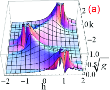
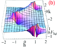
Figure 1: (color online) (a) The gauge invariant $\sqrt{g}$ as a function of $k$ and $h$ ; (b) The Berry curvature $\mathcal{F}_{k\varphi}$ as a function of $k$ and $h$.

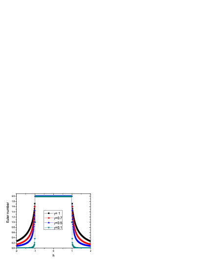
Figure 2: (color online) The Euler number as a characterization of the phase diagram of a transverse field XY spin chain as a function of the transverse field $h$ and the anisotropy parameter $\gamma$.

Here the Riemannian metric is given by

$$\mathcal{G}_{k\varphi}=\frac{1}{4}\left(\begin{array}[]{cc}\frac{\gamma^{2}\left(1+h\cos k\right)^{2}}{\left(h+\cos k\right)^{2}+\gamma^{2}\sin^{2}k}&0\\ 0&\frac{2\gamma^{2}\sin^{2}k}{\left(h+\cos k\right)^{2}+\gamma^{2}\sin^{2}k}\end{array}\right),$$ (7)

and then we can obtain the Ricci scalar $R=8$ by the standard procedures. Finally, the Euler number is given by

$$\chi = \frac{2}{\pi}\int\left|\frac{\bm{\vec{d}}\cdot{\partial_{k}}\bm{\vec{d}}\times{\partial_{\phi}}\bm{\vec{d}}}{d^{3}}\right|dkd\varphi$$ (8)

$$= \int_{0}^{\pi}\sqrt{\frac{\gamma^{4}\left(1+h\cos k\right)^{2}\sin^{2}k}{\left[\left(h+\cos k\right)^{2}+\gamma^{2}\sin^{2}k\right]^{3}}}dk.$$

In Fig. (1), we show the properties of the Berry curvature and the metric tensor in the vicinity of quantum critical points. As expected, both the Berry curvature and metric tensor exhibit singularity around the phase transition points, but as a local quantity, neither of them can serve as a topological order to characterize a topological phase.

As shown in Fig. (2), the ferromagnetic ordered phase in the XY spin chain exhibits a nontrivial even Euler number $\chi=2$, and the Euler number declines rapidly from $2$ to $0$ in the paramagnetic phase. Note that the system is time reversal invariant, so the Berry curvature $\mathcal{F}_{k\varphi}$ is odd with $k$, and the first Chern number, as the integral of the Berry curvature $\mathcal{F}_{k\varphi}$ in the Brillouin zone, is equal to zero. It is clear that the Chern number is not a appropriate topological number for this case. However, it has been pointed out in our recent work Ma2012 that a non trivial $Z_{2}$ number can be obtained as a quantized Berry phase along a loop over half (or quarter) of the Brillouin zone,

$$Z_{2} = \frac{1}{2\pi}\int_{0}^{\pi}d\varphi\int_{0}^{\pi}\frac{\gamma^{2}\left(1+h\cos k\right)\sin k}{\left[\left(h+\cos k\right)^{2}+\gamma^{2}\sin^{2}k\right]^{3/2}}dk$$ (11)

$$= \left\{\begin{array}[]{lll}1,&&\text{if}\quad 0<\left|h\right|<1;\\ 0,&&\text{otherwise.}\end{array}\right..$$

Here, the $Z_{2}$ number is induced by the Berry curvature $\mathcal{F}_{k\varphi}$ ( imaginary part of the geometric tensor) reflecting the topological obstruction of the $U(1)$ principal bundle. In contrast, the Euler number is induced by the Riemannian metric $\mathcal{G}_{k\varphi}$ ( real part of the geometric tensor) of the Bloch state in a (1+1)-dimensional momentum space, which reflects the number of the genus of the Bloch states manifold.

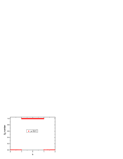
Figure 3: (color online) (Left) The gapless point (red dot) enclosed in the torus is converted into a monopole in the $\bm{d}$-space (Right), and corresponds to a topological sphere of the ground state Riemannian manifold with the Euler number $\chi=2$.

The above results can be understood in an intuitional picture. As shown in Fig. (3), we can see the monopole as a gapless point in the torus in the (1+1)-dimensional momentum space corresponding to the zero point in the three dimensional $\bm{d}$-space. It can be verified that only if $\left|h\right|<1$ then the monopole is enclosed by the surface of $d_{\alpha}\left(k,\varphi\right)$, which corresponds to a topological sphere of the ground state Riemannian manifold with the Euler number $\chi=2$. In this case, the first Chern number is not an effective characterization because of the time reversal invariance, and the $Z_{2}$ number can be expressed as the quantized upper hemispherical flux of the monopole.

V Conclusion

We have introduced the Euler characteristic number $\chi$ as a new topological quantum number to distinguish the topological phase transitions in gapped fermionic systems. In particular, we show that the zero-temperature phase diagram of a transverse field XY spin chain can be characterized by the Euler numbers in the (1+1)-dimensional momentum space. We show that it is the Euler number instead of the Chern number to be an effective characterization of the nontrivial topological phases in the time-reversal invariant systems. This approach provides another description of the topological nature of the ground state in gapped fermionic systems. We hope that this work will raise renewed interest in the understanding of the topological nature in quantum condensed-matter systems.

Note added.— After this manuscript has been submitted, we note that recently a similarly work on the metric tensor and the Euler characteristic number appeared Kolodrubetz .

VI Acknowledgments

This work is supported by the NKBRSFC under grants Nos. 2011CB921502, 2012CB821305, 2010CB922904, 2009CB930701, NSFC under grants Nos. 10934010, 60978019, NSFC-RGC under grants Nos. 11061160490, 1386-N-HKU748/10, and the RGC of HKSAR, China (Project No. HKUST3/CRF/09).

References

• (1) M. V. Berry, Proc. R. Soc. London A 392, 45 (1984).
• (2) B. Simon, Phys. Rev. Lett. 51, 2167 (1983).
• (3) D. J. Thouless, Phys. Rev. B 27, 6083 (1983).
• (4) Q. Niu, Phys. Rev. Lett. 64, 1812 (1990).
• (5) R. B. Laughlin, Phys. Rev. B 23, 5632 (1981).
• (6) D. J. Thouless, M. Kohmoto, M. P. Nightingale and M. den Nijs, Phys. Rev. Lett. 49, 405 (1982).
• (7) Q. Niu and D. J. Thouless, J. Phys. A 17, 2453 (1984).
• (8) C. L. Kane and E. J. Mele, Phys. Rev. Lett. 95, 146802 (2005); 95, 226801 (2005).
• (9) L. Fu, C. L. Kane, and E. J. Mele, Phys. Rev. Lett. 98, 106803 (2007).
• (10) M. Z. Hasan and C. L. Kane, Rev. Mod. Phys. 82, 3045 (2010).
• (11) X. L. Qi and S. C. Zhang, Rev. Mod. Phys. 83, 1057 (2011).
• (12) J. P. Provost and G. Vallee, Commun. Math. Phys. 76. 289 (1980).
• (13) M. V. Berry, in Geometric Phases in Physics, edited by A. Shapere and F. Wilczek (World Scientific, Singapore, 1989).
• (14) R. Resta, Phys. Rev. Lett. 95, 196805 (2005).
• (15) F. D. M. Haldane, Phys. Rev. Lett. 107, 116801 (2011).
• (16) Y. Q. Ma, S. Chen, H. Fan, and W. M. Liu, Phys. Rev. B 81, 245129 (2010).
• (17) S. Matsuura and S. Ryu, Phys. Rev. B 82, 245113 (2010).
• (18) A. T. Rezakhani, D. F. Abasto, D. A. Lidar, and P. Zanardi, Phys. Rev. A 82, 012321 (2010).
• (19) S. Sachdev, Quantum Phase Transitions (Cambridge University Press, Cambridge, UK, 2000).
• (20) P. Zanardi, P. Giorda and M. Cozzini, Phys. Rev. Lett. 99, 100603 (2007).
• (21) L. C. Venuti and P. Zanardi, Phys. Rev. Lett. 99, 095701 (2007).
• (22) S. J. Gu, Int. J. Mod. Phys. B, 24, 4371 (2010).
• (23) W. L. You, Y. W. Li and S. J. Gu, Phys. Rev. E 76, 022101 (2007).
• (24) A. C. M. Carollo and J. K. Pachos, Phys. Rev. Lett. 95, 157203 (2005).
• (25) A. Hamma, arXiv: quant-ph/0602091 (2006).
• (26) S. L. Zhu, Phys. Rev. Lett. 96, 077206 (2006).
• (27) Y. Q. Ma and S. Chen, Phys. Rev. A 79, 022116 (2009).
• (28) X. G. Wen, Quantum Field Theory of Many-Body Systems (Oxford University, New York, 2004).
• (29) D. F. Abasto, A. Hamma, and P. Zanardi, Phys. Rev. A 78, 010301 (2008).
• (30) S. Yang, S. J. Gu, C. P. Sun, and H. Q. Lin, Phys. Rev. A 78, 012304 (2008).
• (31) A. Hamma, W. Zhang, S. Haas, and D. A. Lidar, Phys. Rev. B 77, 155111 (2008).
• (32) S. Garnerone, D. Abasto, S. Haas, and P. Zanardi, Phys. Rev. A 79, 032302 (2009).
• (33) T. Hirano, H. Katsura, and Y. Hatsugai, Phys. Rev. B 77, 094431 (2008); Y. Hatsugai, New J. Phys. 12, 065004 (2010).
• (34) T. Fukui and T. Fujiwara, J.Phys.Soc.Jpn. 78, 093001 (2009).
• (35) Y. Q. Ma, et. al., EPL, 100, 60001 (2012).
• (36) M. Kolodrubetz, V. Gritsev, A. Polkovnikov, arXiv:1305.0568, (2013).