A revised asteroid polarization-albedo relationship using WISE/NEOWISE data

Abstract

We present a reanalysis of the relationship between asteroid albedo and polarization properties using the albedos derived from the Wide-field Infrared Survey Explorer. We find that the function that best describes this relation is a three-dimensional linear fit in the space of $\log$ (albedo)-$\log$ (polarization slope)-$\log$ (minimum polarization). When projected to two dimensions the parameters of the fit are consistent with those found in previous work. We also define $p^{\star}$ as the quantity of maximal polarization variation when compared with albedo and present the best fitting albedo-$p^{\star}$ relation. Some asteroid taxonomic types stand out in this three-dimensional space, notably the E, B, and M Tholen types, while others cluster in clumps coincident with the S- and C-complex bodies. We note that both low albedo and small ($D<30~{}$km) asteroids are under-represented in the polarimetric sample, and we encourage future polarimetric surveys to focus on these bodies.

1 Introduction

As light scatters off the surface of atmosphereless bodies, it is instilled with a small linear polarization. The degree of linear polarization of the scattered light measured by the observer is a function of the phase angle of observation and the composition and structure of the surface, in particular the interrelated parameters of albedo, index of refraction, and space between scattering elements (e.g. Muinonen, 1989; Shkuratov et al., 1994). Early work quantified the relation between phase angle (the angle between the direction to the sun and the observer as seen from the target, $\alpha$) and polarization (Dollfus & Zellner, 1979) and this effect can be used in parallel with the magnitude-phase effect to probe the scattering physics of atmosphereless surfaces (Muinonen et al., 2002, 2009).

As expected from classical scattering models, the light reflected from a surface is polarized perpendicular to the scattering plane for large phase angles, which is referred to as a positive polarization. For small phase angles, however, light acquires a polarization in the scattering plane due to an increase in the dominance of second-order scattering. This case is referred to as negative polarization, as it is perpendicular to the positive case and thus carries a negative sign when the polarization coordinate system is rotated to account for the viewing geometry. The angle where the phase curve transitions from positive to negative is referred to as the inversion angle ($\alpha_{0}$). By definition the value of the polarization must go to zero at $\alpha=0^{\circ}$, though some work has suggested that surfaces may have a secondary trough at very small angles related to the optical opposition effect (Rosenbush et al., 1997). Cellino et al. (2005a) find no evidence for a polarimetric opposition effect in their sample, though high albedo objects are not represented there.

From the studies of the scattering properties of the lunar surface, a relationship was found between albedo and the parameters used to describe the polarimetric-phase effect of the lunar regolith (Bowell et al., 1973) that was then extended to asteroids (Zellner et al., 1974; Cellino et al., 1999), of the form:

$$\log p_{V}=C_{1}\log h+C_{2}$$ (1)

$$\log p_{V}=C_{3}\log P_{min}+C_{4}$$ (2)

where $p_{V}$ is the geometric albedo, $h$ is the linear slope of the phase curve at the inversion angle, and $P_{min}$ is the value of the largest negative polarization (i.e. the depth of the negative trough), usually expressed as an absolute value. We show an illustration of these parameters and two typical polarization-phase curves in Figure 1. We note that the polarization shown in this figure is the $P_{r}$ value that has been rotated to account for viewing geometry, such that $P_{r}>0$ is the amplitude of polarization perpendicular to the scattering plane and $P_{r}<0$ is the amplitude parallel to the scattering plane. A polarization component $\pm 45^{\circ}$ from the scattering plane is typically not observed at any phase angle for asteroids, and thus is ignored in this diagram.

Cellino et al. (1999) present the most recent best-fitting values for the constants in the above equations: $C_{1}=-1.118\pm 0.071$, $C_{2}=-1.779\pm 0.062$, $C_{3}=-1.357\pm 0.140$, and $C_{4}=-0.858\pm 0.030$. In this work, we revise the best-fitting values for these constants in light of new albedo data from the Wide-field Infrared Survey Explorer (WISE, Wright et al., 2010) and the planetary science extension NEOWISE (Mainzer et al., 2011a). The aim of this work is two-fold: firstly, while WISE provides us with albedos for a large fraction of the known asteroids, calibration of this relationship will allow it to be applied to objects that were not observed by WISE; secondly, the behavior of the polarization of asteroid surfaces helps us determine the surface mineralogy and this relationship represents a critical component in this determination. Through application of both thermal infrared and polarimetric data we can gain a broader understanding of the behavior of asteroids across the Solar system.

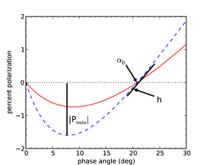
Figure 1: Illustration of the typical polarization-phase behavior for two different types of asteroids, with the inversion angle ($\alpha_{0}$), the minimum polarization ($P_{min}$), and the slope of polarization at the inversion angle ($h$) labeled for the dashed blue curve. Example curves for a generic S-type asteroid (solid red line) and a generic C-type (dashed blue line) are shown.

2 Data

We draw our list of polarimetric properties for asteroids from a range of sources. The dominant contributor is the Astronomical Polarimetric Database presented in the Planetary Data System (PDS) (Lupishko & Vasilyev, 2008) which was a compilation of the polarimetric properties of individual asteroids in the literature up to the data of publication. We also incorporate values for $h$, $P_{min}$, and/or $\alpha_{0}$ for asteroids given by: Cellino et al. (1999, 2005a, 2005b); Fornasier et al. (2006); Gil-Hutton (2007a); Gil-Hutton et al. (2007b, 2008); Masiero & Cellino (2009); Belskaya et al. (2010). We note that as these data are drawn from a range of different instruments, uncertainties in the absolute calibration may result in a larger scatter than is actually present. A comprehensive survey of polarimetric properties of a large number of objects conducted with a single instrument would reduce this possible source of error, and so is strongly encouraged.

Determination of $h$, $P_{min}$, and $\alpha_{0}$ all require polarimetric measurements spanning a range of phase angles. The inversion angle can typically be determined to a reasonable level of accuracy with a few bounding measurements at $\alpha\sim 20^{\circ}$. Polarimetric slope is more difficult to determine, especially for objects located farther from the sun that are rarely observable at phase angles much beyond the inversion angle (e.g. objects that do not come within $\sim 2.9~{}$AU of the sun can never be observed at phase angles $\alpha>20^{\circ}$). Careful timing of observations can ensure adequate phase coverage that will allow for an accurate determination of the slope. The depth of minimum polarization is often the most difficult parameter to determine for some objects, as it requires observing at small phase angles that are not frequently available for asteroids in the inner Main Belt, Hungaria, Mars Crosser, and NEO populations. Additionally, determining this value requires evenly spaced observations over the full branch of negative polarization, rather than just a few bounding measurements as required for both $\alpha_{0}$ and $h$. As such, relative errors on $P_{min}$ tend to be larger than measured for the other polarimetric parameters. Where errors on polarimetric parameters were not given by the source, we assume values based on the errors on the published data in those sources.

The albedos we use for this work are drawn from the values derived for Main Belt asteroids (MBAs) published in Masiero et al. (2011). For objects in the NEO or Mars Crossing populations, we draw albedos from the appropriate lists (Mainzer et al., 2011e, f) which were derived using a method identical to that used for the MBAs. All of the objects with both defined polarimetric phase curves as well as WISE-determined albedos had low identifying numbers, implying that they were some of the first objects discovered, and thus likely to preferentially sample the largest minor bodies of the solar system. These large asteroids were more likely to have been seen in multiple bands by WISE which allows for fitting of the beaming parameter. Mainzer et al. (2011b) show that in cases such as this the error on albedo as an absolute measurement is $\sim 20\%$ of the measured albedo value, however internal comparisons are better than this limit.

A primary concern in any analysis of albedos derived from infrared-determined diameters is the quality of the optical measurements used. We draw our $H$ magnitudes from the Minor Planet Center’s orbital element catalog (MPCORB), as discussed in Masiero et al. (2011). While other studies have found an offset between measured magnitudes and those predicted from the $H$ absolute magnitude value, with objects being fainter than expected (e.g. Jurić et al., 2002; Parker et al., 2008), Mainzer et al. (2011b) find that, in general, no offset corrections to $H$ are required for the most recent releases of the magnitudes. An exception to this result has been found for some objects with unusually high albedos in Masiero et al. (2011) and Mainzer et al. (2011e); many of these objects are coincident in orbital-element-space with the Hungarias and the Vesta family. Harris et al. (1989) found that the commonly assumed value of $G=0.15$ is inappropriate for these types of high-albedo objects, and a value of $G\sim 0.4$ may be more appropriate. Revising $G$ to this value would result in an offset of up to $\sim 0.3~{}$mag in the $H$ magnitude depending on the initial $H$ fit, however this correction is not required for most objects. In the past, photometric measurements for many asteroids that contributed to the $H$ magnitudes in the MPCORB catalog were acquired with unfiltered CCDs. New, filtered observations and refined handling of previous photometry have largely mitigated the effect of unfiltered measurements on $H$ values. (T. Spahr, 2012, private communication).

Mainzer et al. (2011c) present a comparison of the WISE albedos to the IRAS albedos and find a good match for most objects, though some scatter is seen, especially at the smallest sizes where the IRAS signal-to-noise ratios were poor compared to WISE. This albedo error assumes moderate-to-low light curve amplitudes and well characterized $H$ and $G$ values. This error will result in an uncertainty in the offsets of the linear fits (i.e. $C_{2}$ and $C_{4}$ in Equations 1 and 2) though the slopes should be unaffected. We include this error in our fits below. We note that recently Muinonen et al. (2010) have introduced a three-parameter photometric system ($H$,$G_{1}$,$G_{2}$) to better characterize the behavior of the photometric phase effect which may reduce some of these errors, but we note that this system requires accurate photometry over a large phase window, which is not available for many asteroids.

We show the polarimetric and albedo data used for this work in Table LABEL:tab.data (ellipses indicate an unmeasured polarimetric property). When these two data sets are combined, we have $65$ objects with measured albedos and polarimetric slopes, and $112$ with albedos and minimum polarization values. This result is a improvement compared to the data set presented by Cellino et al. (1999), who performed a similar analysis using IRAS albedos of $37$ objects for the slope-albedo fit and $16$ for the minimum polarization-albedo fit. We note that due to the brightness requirements of most polarimeters and the polarimetric survey strategies employed, these lists are dominated by the largest known asteroids. Approximately half our sample have sizes over $100~{}$km, and three-quarters are larger than $50~{}$km. Thus while the largest asteroids are well sampled, there is a distinct lack of small bodies in these lists. We also note that despite the fact that low-albedo objects dominate the Main Belt population (Masiero et al., 2011), they are under-represented in the polarimetric surveys (see below). As WISE is sensitive to thermal infrared light, the detection probability for asteroids is effectively unbiased with respect to the albedos of the objects observed (Mainzer et al., 2011e), and thus the distribution of albedos seen with WISE is a more accurate representation of the true population than is the distribution seen for optically-selected samples. Extending polarimetric coverage to both smaller sizes and low albedo objects through a large-scale campaign is critical to extending and generalizing the trends seen here and in previous work.

Table 1: Compiled asteroid albedos and polarimetric properties

Asteroid	$p_{V}$	$\alpha_{0}$	$h$	$P_{min}$
2	$0.142\pm 0.018$	$18.1\pm 0.1$	$0.228\pm 0.003$	$1.38\pm 0.05$
5	$0.245\pm 0.051$	$19.1\pm 0.1$	$0.096\pm 0.050$	$0.70\pm 0.05$
6	$0.269\pm 0.049$	$20.8\pm 0.2$	$0.091\pm 0.050$	$0.80\pm 0.05$
8	$0.261\pm 0.048$	$20.0\pm 0.1$	$0.104\pm 0.003$	$0.68\pm 0.05$
9	$0.134\pm 0.016$	$21.8\pm 0.1$	$0.102\pm 0.003$	$0.74\pm 0.05$
10	$0.058\pm 0.005$	$...$	$...$	$1.50\pm 0.05$
11	$0.158\pm 0.036$	$18.9\pm 0.2$	$0.124\pm 0.003$	$0.73\pm 0.05$
12	$0.140\pm 0.014$	$20.8\pm 0.2$	$0.121\pm 0.003$	$0.73\pm 0.01$
13	$0.069\pm 0.022$	$21.7\pm 0.5$	$0.257\pm 0.003$	$2.10\pm 0.05$
14	$0.221\pm 0.022$	$20.5\pm 0.2$	$0.105\pm 0.003$	$0.82\pm 0.10$
15	$0.206\pm 0.055$	$20.6\pm 0.2$	$0.087\pm 0.005$	$0.72\pm 0.02$
17	$0.160\pm 0.009$	$...$	$0.131\pm 0.003$	$0.74\pm 0.05$
18	$0.221\pm 0.082$	$21.6\pm 0.1$	$0.101\pm 0.003$	$0.87\pm 0.05$
19	$0.050\pm 0.020$	$21.7\pm 0.2$	$0.305\pm 0.003$	$1.72\pm 0.05$
22	$0.169\pm 0.061$	$...$	$...$	$0.83\pm 0.04$
24	$0.064\pm 0.016$	$...$	$0.191\pm 0.003$	$1.63\pm 0.10$
27	$0.201\pm 0.058$	$...$	$0.099\pm 0.003$	$0.70\pm 0.05$
29	$0.157\pm 0.035$	$22.0\pm 0.2$	$0.098\pm 0.003$	$0.88\pm 0.10$
30	$0.171\pm 0.034$	$19.8\pm 0.5$	$0.104\pm 0.003$	$0.78\pm 0.05$
31	$0.045\pm 0.044$	$...$	$...$	$1.32\pm 0.10$
32	$0.230\pm 0.065$	$...$	$...$	$0.63\pm 0.05$
39	$0.245\pm 0.056$	$21.0\pm 0.1$	$0.090\pm 0.003$	$0.79\pm 0.05$
40	$0.195\pm 0.019$	$20.8\pm 0.2$	$0.100\pm 0.003$	$0.85\pm 0.05$
46	$0.052\pm 0.011$	$...$	$...$	$1.54\pm 0.10$
47	$0.067\pm 0.009$	$...$	$0.204\pm 0.003$	$1.44\pm 0.05$
51	$0.100\pm 0.026$	$...$	$0.292\pm 0.050$	$1.86\pm 0.05$
54	$0.049\pm 0.008$	$22.2\pm 0.5$	$0.357\pm 0.050$	$1.95\pm 0.05$
56	$0.050\pm 0.006$	$19.7\pm 0.2$	$0.318\pm 0.003$	$1.47\pm 0.05$
57	$0.182\pm 0.047$	$...$	$...$	$0.71\pm 0.10$
58	$0.059\pm 0.005$	$...$	$...$	$1.70\pm 0.10$
63	$0.159\pm 0.028$	$19.8\pm 0.1$	$0.102\pm 0.003$	$0.70\pm 0.05$
64	$0.676\pm 0.223$	$18.2\pm 0.2$	$0.036\pm 0.001$	$0.32\pm 0.05$
68	$0.207\pm 0.025$	$...$	$...$	$0.68\pm 0.05$
70	$0.040\pm 0.009$	$...$	$...$	$1.83\pm 0.05$
71	$0.248\pm 0.035$	$...$	$0.061\pm 0.005$	$0.61\pm 0.02$
73	$0.186\pm 0.018$	$...$	$...$	$0.76\pm 0.06$
75	$0.098\pm 0.014$	$20.2\pm 0.1$	$0.103\pm 0.017$	$...$
77	$0.153\pm 0.046$	$...$	$...$	$1.25\pm 0.14$
80	$0.182\pm 0.026$	$...$	$...$	$0.75\pm 0.05$
83	$0.086\pm 0.021$	$...$	$...$	$1.47\pm 0.10$
84	$0.053\pm 0.017$	$20.3\pm 0.5$	$0.306\pm 0.050$	$1.49\pm 0.05$
85	$0.063\pm 0.025$	$...$	$...$	$1.36\pm 0.10$
89	$0.185\pm 0.034$	$...$	$0.119\pm 0.050$	$0.90\pm 0.05$
95	$0.056\pm 0.009$	$...$	$...$	$1.78\pm 0.05$
97	$0.206\pm 0.046$	$22.1\pm 0.1$	$0.174\pm 0.018$	$...$
113	$0.223\pm 0.031$	$...$	$0.081\pm 0.005$	$...$
114	$0.088\pm 0.010$	$...$	$...$	$1.24\pm 0.10$
115	$0.654\pm 0.124$	$...$	$...$	$0.71\pm 0.05$
118	$0.139\pm 0.031$	$...$	$...$	$0.80\pm 0.12$
121	$0.077\pm 0.010$	$...$	$...$	$1.72\pm 0.05$
125	$0.115\pm 0.027$	$...$	$0.145\pm 0.033$	$0.83\pm 0.02$
129	$0.157\pm 0.026$	$...$	$...$	$0.90\pm 0.05$
131	$0.164\pm 0.011$	$...$	$0.208\pm 0.059$	$...$
132	$0.120\pm 0.008$	$...$	$0.146\pm 0.006$	$1.13\pm 0.03$
135	$0.152\pm 0.050$	$...$	$...$	$1.06\pm 0.10$
138	$0.161\pm 0.028$	$...$	$0.103\pm 0.020$	$...$
139	$0.045\pm 0.023$	$...$	$0.262\pm 0.050$	$1.31\pm 0.05$
141	$0.049\pm 0.010$	$20.6\pm 0.5$	$0.330\pm 0.050$	$1.78\pm 0.05$
145	$0.043\pm 0.004$	$...$	$...$	$1.86\pm 0.05$
153	$0.046\pm 0.008$	$...$	$...$	$1.05\pm 0.05$
182	$0.210\pm 0.059$	$...$	$...$	$0.64\pm 0.05$
184	$0.107\pm 0.019$	$...$	$...$	$0.93\pm 0.06$
188	$0.157\pm 0.055$	$...$	$0.140\pm 0.015$	$...$
189	$0.199\pm 0.024$	$...$	$...$	$1.26\pm 0.10$
192	$0.288\pm 0.040$	$19.8\pm 0.1$	$0.084\pm 0.003$	$0.75\pm 0.05$
197	$0.239\pm 0.026$	$...$	$...$	$0.79\pm 0.08$
201	$0.097\pm 0.006$	$...$	$...$	$1.00\pm 0.05$
204	$0.163\pm 0.044$	$...$	$...$	$0.83\pm 0.12$
216	$0.111\pm 0.034$	$...$	$...$	$1.27\pm 0.05$
217	$0.044\pm 0.005$	$...$	$...$	$0.82\pm 0.05$
230	$0.171\pm 0.076$	$20.6\pm 0.2$	$0.122\pm 0.003$	$0.94\pm 0.05$
234	$0.151\pm 0.034$	$27.0\pm 2.0$	$...$	$1.60\pm 0.20$
250	$0.112\pm 0.021$	$...$	$...$	$0.88\pm 0.08$
259	$0.042\pm 0.005$	$...$	$...$	$1.25\pm 0.05$
270	$0.254\pm 0.043$	$...$	$...$	$0.65\pm 0.05$
305	$0.182\pm 0.028$	$...$	$...$	$0.64\pm 0.10$
306	$0.174\pm 0.060$	$...$	$...$	$0.66\pm 0.10$
324	$0.063\pm 0.012$	$20.0\pm 0.1$	$0.278\pm 0.003$	$1.46\pm 0.05$
334	$0.051\pm 0.016$	$...$	$...$	$1.32\pm 0.05$
338	$0.165\pm 0.028$	$...$	$...$	$0.98\pm 0.10$
345	$0.059\pm 0.012$	$...$	$...$	$1.55\pm 0.05$
347	$0.213\pm 0.041$	$22.6\pm 0.1$	$0.113\pm 0.003$	$0.78\pm 0.03$
349	$0.153\pm 0.018$	$...$	$...$	$0.39\pm 0.05$
351	$0.171\pm 0.046$	$...$	$...$	$0.74\pm 0.09$
354	$0.173\pm 0.032$	$...$	$...$	$0.51\pm 0.10$
356	$0.053\pm 0.015$	$...$	$...$	$1.50\pm 0.10$
377	$0.056\pm 0.025$	$19.8\pm 0.2$	$0.206\pm 0.005$	$1.76\pm 0.04$
384	$0.190\pm 0.040$	$...$	$...$	$0.94\pm 0.35$
396	$0.139\pm 0.025$	$...$	$...$	$1.34\pm 0.09$
409	$0.050\pm 0.010$	$19.9\pm 0.2$	$0.191\pm 0.005$	$...$
410	$0.043\pm 0.007$	$...$	$0.313\pm 0.050$	$1.94\pm 0.05$
415	$0.086\pm 0.009$	$...$	$...$	$1.28\pm 0.10$
423	$0.066\pm 0.005$	$...$	$...$	$1.40\pm 0.05$
441	$0.139\pm 0.026$	$...$	$...$	$1.41\pm 0.12$
451	$0.069\pm 0.006$	$...$	$...$	$1.62\pm 0.05$
466	$0.086\pm 0.009$	$...$	$...$	$1.60\pm 0.10$
511	$0.073\pm 0.006$	$19.4\pm 0.1$	$0.277\pm 0.003$	$1.69\pm 0.05$
532	$0.202\pm 0.039$	$...$	$0.122\pm 0.003$	$0.78\pm 0.05$
550	$0.137\pm 0.024$	$...$	$0.157\pm 0.005$	$...$
558	$0.117\pm 0.010$	$...$	$...$	$0.75\pm 0.06$
584	$0.244\pm 0.060$	$19.1\pm 0.1$	$0.108\pm 0.003$	$0.64\pm 0.05$
600	$0.177\pm 0.036$	$...$	$...$	$0.43\pm 0.20$
602	$0.052\pm 0.007$	$...$	$...$	$1.76\pm 0.10$
624	$0.077\pm 0.020$	$...$	$...$	$1.30\pm 0.05$
625	$0.197\pm 0.058$	$...$	$0.070\pm 0.003$	$...$
654	$0.043\pm 0.011$	$20.5\pm 0.5$	$0.280\pm 0.050$	$1.46\pm 0.10$
662	$0.193\pm 0.028$	$...$	$...$	$1.32\pm 0.33$
674	$0.206\pm 0.033$	$...$	$...$	$0.81\pm 0.10$
704	$0.076\pm 0.010$	$15.7\pm 0.1$	$0.305\pm 0.003$	$1.45\pm 0.10$
737	$0.136\pm 0.043$	$...$	$...$	$0.84\pm 0.05$
787	$0.120\pm 0.022$	$...$	$0.087\pm 0.003$	$...$
796	$0.205\pm 0.041$	$...$	$0.124\pm 0.011$	$0.98\pm 0.02$
849	$0.115\pm 0.016$	$...$	$...$	$0.95\pm 0.05$
857	$0.225\pm 0.026$	$...$	$...$	$0.75\pm 0.16$
863	$0.112\pm 0.016$	$18.1\pm 0.2$	$0.052\pm 0.005$	$0.40\pm 0.10$
887	$0.230\pm 0.018$	$...$	$0.101\pm 0.050$	$0.76\pm 0.05$
925	$0.253\pm 0.053$	$19.6\pm 0.2$	$0.065\pm 0.005$	$...$
1036	$0.212\pm 0.026$	$20.6\pm 0.2$	$0.112\pm 0.003$	$0.84\pm 0.02$
1052	$0.273\pm 0.074$	$...$	$...$	$0.67\pm 0.05$
1058	$0.242\pm 0.024$	$...$	$...$	$0.69\pm 0.10$
1105	$0.102\pm 0.017$	$...$	$...$	$1.20\pm 0.16$
1355	$0.466\pm 0.082$	$18.2\pm 0.1$	$0.083\pm 0.020$	$...$
1627	$0.153\pm 0.046$	$...$	$0.131\pm 0.003$	$...$
1672	$0.094\pm 0.016$	$...$	$0.131\pm 0.003$	$...$
1685	$0.292\pm 0.127$	$...$	$0.099\pm 0.003$	$...$
2131	$0.198\pm 0.034$	$...$	$...$	$0.86\pm 0.15$
2577	$0.377\pm 0.062$	$20.9\pm 0.1$	$0.124\pm 0.044$	$...$
3169	$0.423\pm 0.067$	$19.6\pm 0.1$	$0.276\pm 0.018$	$...$
6249	$0.878\pm 0.140$	$22.4\pm 0.1$	$0.164\pm 0.035$	$...$
6911	$0.454\pm 0.083$	$...$	$...$	$0.83\pm 0.16$

Table 1: (continued)

3 Revised Polarimetric-Albedo Relationship

In Figures 2-4 we compare the measured WISE albedo to the slope of the polarization beyond the inversion angle, the depth of the negative branch of polarization, and the inversion angle, respectively, for all objects with recorded values for these parameters. We distinguish objects in the Hungaria region and in the NEO population as red squares and cyan triangles, respectively. While the NEOs appear consistent with the MBAs, the Hungaria objects deviate from the general trend significantly. As discussed in Masiero et al. (2011) the albedos for these objects are suspect: large deviations in the magnitude-phase slope parameter from the assumed $G=0.15$ used for most asteroids can result in incorrect $H$ values, and thus poorly constrained albedos (Harris et al., 1989). Alternatively, large-amplitude long-period light curves may also corrupt the $H$ values calculated from optical photometry. We are currently working on a program to better constrain the photometric parameters and albedos of these objects, but for the following discussion we will disregard the Hungaria asteroids.

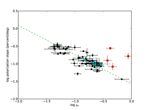
Figure 2: Albedo vs. slope of the polarization phase curve beyond the inversion angle. Objects located in the Hungaria region are noted as red squares, objects in the NEO population as cyan triangles. The green dashed line shows the best fit found for Equation 1 with our data.

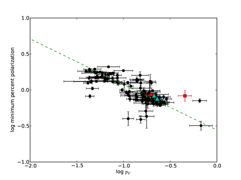
Figure 3: The same as Figure 2, but for albedo vs. depth of the minimum polarization branch. The green dashed line shows the best fit found for Equation 2 with our data.

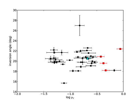
Figure 4: The same as Figure 2, but for albedo vs. inversion angle.

We see no overall trend between albedo and inversion angle in our data. The object with the anomalously high inversion angle is (234) Barbara, the principal member of the “Barbarian” group of objects with strange polarimetric properties (Cellino et al., 2006). The object with an inversion angle well below the general trend is (704) Interamnia: some F-class objects like Interamnia have previously been shown to display unusually small inversion angles (Belskaya et al., 2005).

We see the expected general trends when looking at slope and P_min, with low albedo objects showing steeper slopes and deeper troughs. We note, however, that the lowest albedo objects, those with $p_{V}<0.04$, have almost no representation in the polarimetric sample despite representing over $10\%$ of the total population of MBAs observed by WISE, even before correcting the population for objects without optical followup (and thus without measured albedos). We therefore cannot comment on the reliability of the polarization-phase relation at the lowest albedos. A campaign of polarimetric observations of low albedo asteroids is critical to test these relations at their low albedo extreme.

We find that the optimal description of the relation between albedo and polarimetric parameters is a linear fit in the three dimensional space of $\log p_{V}$-$\log h$-$\log P_{min}$. We use only those objects where both polarimetric parameters are measured to an accuracy of $20\%$ or better, leaving us with $41$ objects in our high-confidence sample. We perform orthogonal distance regression on the three dimensional data, using the associated errors on each measurement to determine the best fitting linear parameters as well as each parameter’s error. We then reduce the best-fit parameters back to two-dimensional projections, which result in the following constant parameters for the relationships in Equations 1 and 2:

$$C_{1}=-1.207\pm 0.067$$

$$C_{2}=-1.892\pm 0.141$$

$$C_{3}=-1.579\pm 0.084$$

$$C_{4}=-0.880\pm 0.106$$

These projected fits are shown as green dashed lines in Figures 2 and 3. With the exception of $C_{3}$, these parameters are all within one-sigma of the values found by Cellino et al. (1999), and all are within 1.5 sigma. As the WISE albedos for the largest asteroids have been shown to be generally consistent with the IRAS values (Mainzer et al., 2011c) and all of the objects used here are in the size range sampled by IRAS, this agreement was not unexpected. Of the objects in our high-confidence polarimetric sample only $6$ were not observed by IRAS, however the WISE albedos are all derived from a minimum of $5$ observations (and an average of $>10$) spread over time and thus are less sensitive to rotation effects. As the WISE data cover MBAs down to a few kilometers and NEOs to much smaller sizes, future polarimetric surveys focusing on smaller asteroids will allow this relationship to be tested over a more extensive size range.

We can also project our fit of the polarimetric properties onto an axis of maximal variation. We define $p^{\star}$ as the quantity of maximum polarimetric variation and find a best-fitting transform of:

$$p^{\star}=(0.79\pm 0.02)\log h+(0.61\pm 0.03)\log P_{min}$$

Using our data we find a best-fitting relation between $p^{\star}$ and albedo of:

$$\log p_{V}=(-1.58\pm 0.09)+(-1.04\pm 0.04)p^{\star}$$

We show $p^{\star}$ compared to albedo for all of the high-confidence objects with both measured $h$ and $P_{min}$, along with this fit, in Figure 5. We label (64) Angelina as “E”, (2) Pallas as “B”, and (132) Aethra as “M” following their Tholen taxonomic classifications (Neese, 2010). The clusters of objects with Tholen S and C taxonomic classifications are labeled as such, and include other objects within those taxonomic complexes (e.g. F- and D-types are included in the C-complex) . We indicate (71) Niobe with “n” in this plot; though it has a Tholen class of S it is distinct enough from the general cluster to warrant mention. Additional polarimetric and spectroscopic followup of this object will help determine why its properties differ from the general S complex. We focus on Tholen classifications here as this taxonomic system shows the greatest distinction in albedo between the different types (Mainzer et al., 2011d).

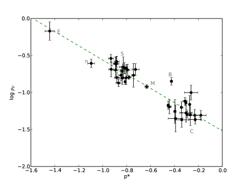
Figure 5: The maximal variation of the polarimetric properties $p^{\star}$ as defined in the text compared to the measured albedo. The best-fitting relationship projected from the three-dimensional fit is shown as the dashed line. Text labels denote specific asteroids or groupings as discussed in the text.

In addition to the lack of the lowest albedo objects in the polarimetric sample, we observe an over-representation of high albedo objects compared to the distribution for all similarly sized MBAs. Figure 6 shows the distribution of albedos of all objects in the sample with high-confidence polarimetric properties used to derive the linear three dimensional fit (the smallest of which is $D\sim 35~{}$km), as well as all MBAs larger than $30~{}$km in diameter that were observed by WISE. The difference in these two distributions can be traced to the optical selection bias in the acquisition and measurement of the polarimetric properties of asteroids: very high signal-to-noise levels are needed to reach the polarimetric sensitivities that allow for accurate measurement of $P_{min}$ and $h$. Thus, even though at a given phase angle low albedo objects will show larger degrees of polarization, the reduction in photons received from these sources make these measurements less precise. Focusing future polarimetric surveys on low albedo asteroids will help make this sample more representative of the true distribution of MBAs.

Figure 6: Normalized albedo distribution of the high-confidence polarimetric sample (solid) and all MBAs larger than $30~{}$km that were detected during the fully cryogenic portion of the NEOWISE survey (dotted).

4 Conclusions

Using the newly available albedos from the WISE space telescope thermal infrared survey data, we have fit the relationships between albedo, the slope of the polarimetric-phase curve beyond the inversion angle, and the maximum depth of the negative polarization trough. We restrict ourselves to objects with well characterized polarimetric properties (i.e. relative errors $<20\%$). Due to the selection of the polarimetrically observed objects this results in our sample consisting of only objects larger than $D>30~{}$km, with nearly three-quarters having $D>50~{}$km.

We find that the function that best describes the albedo and polarimetry is a three dimensional linear fit in $\log p_{V}$-$\log h$-$\log P_{min}$ space. Orthogonal distance regression allows us to find the best fitting parameters while accounting for measurement error on all parameters. When the best fit line is projected to two dimensions, we find the resultant fit parameters are all within $1.5$ sigma of those found by Cellino et al. (1999). We also define a new polarimetric quantity $p^{\star}$ that describes the maximum variation in polarimetric properties when compared with albedo.

We observe distinct separation of some taxonomic classes in $p^{\star}$ space. In particular E-type, B-type, and some M-type asteroids are far removed from the clumps that trace the more generic S- and C-complex objects. Asteroid (71) Niobe also holds a distinct location in this space despite its S-type classification under the Tholen system, and warrants further study. We note that the principal component (PC) analysis of Niobe from the Eight Color Asteroid Survey indicates that it is on the edge of the S-complex (Tholen, 1984) and it has a PC4 in the bottom two percent of all asteroids in that survey (one of only 3 S-type or probable S-type objects with PC4 that low Zellner et al., 2009).

Finally, despite the prevalence of low albedo asteroids seen throughout the Main Belt (Masiero et al., 2011) we find that they are under-represented in the polarimetric sample. Notably, roughly $10\%$ of MBAs have albedos $p_{V}<0.04$, but there are no objects in our polarimetric sample with albedos this low. We recommend that future surveys focus on measuring polarization-phase curves for low albedo asteroids to properly sample this population.

References

- Belskaya et al. (2005) Belskaya, I.N., Shkuratov, Yu.G., Efimov, Yu.S., et al., 2005, Icarus, 178, 213.
- Belskaya et al. (2010) Belskaya, I.N., Fornasier, S., Krugly, Yu.N., et al., 2010, A&A, 515, 29.
- Bowell et al. (1973) Bowell, E., Dollfus, A., Zellner, B. & Geake, J.E., 1973, Proc. of the Lunar Science Conference, 4, 3167.
- Cellino et al. (1999) Cellino, A., Gil Hutton, R., Tedesco, E.F., di Martino, M. & Brunini, A., 1999, Icarus, 138, 129.
- Cellino et al. (2005a) Cellino, A., Gil Hutton, R., di Martino, M., Bendjoya, Ph., Belskaya, I.N. & Tedesco, E.F., 2005a, Icarus, 179, 304.
- Cellino et al. (2005b) Cellino, A., Yoshida, F., Anderlucci, E., et al., 2005b, Icarus, 179, 297.
- Cellino et al. (2006) Cellino, A., Belskaya, I.N., Bendjoya, Ph., et al., 2006, Icarus, 180, 565.
- Dollfus & Zellner (1979) Dollfus, A. & Zellner, B., 1979, Asteroids (Univ of Arizona Press), 170.
- Fornasier et al. (2006) Fornasier, S., Belskaya, I.N., Shkuratov, Yu.G., et al., 2006, A&A, 455, 371.
- Gil-Hutton (2007a) Gil-Hutton, R., 2007a, A&A, 464, 1127.
- Gil-Hutton et al. (2007b) Gil-Hutton, R., Lazzaro, D. & Benavidez, P., 2007b, A&A, 468, 1109.
- Gil-Hutton et al. (2008) Gil-Hutton, R., Mesa, V., Cellino, A. et al., 2008, A&A, 482, 309.
- Harris et al. (1989) Harris, A.W., Young, J.W., Contreiras, L. et al., 1989, Icarus, 81, 365.
- Jurić et al. (2002) Jurić, M., Ivezić, Z̆., Lupton, R.H., et al., 2002, AJ, 124, 1776.
- Lupishko & Vasilyev (2008) Lupishko, D.F. and Vasilyev, S.V., Eds., Asteroid Polarimetric Database V6.0. EAR-A-3-RDR-APD-POLARIMETRY-V6.0. NASA Planetary Data System, 2008.
- Mainzer et al. (2011a) Mainzer, A.K., Bauer, J.M., Grav, T., Masiero, J., Cutri, R.M., Dailey, J., Eisenhardt, P., McMillan, R.M. et al., 2011a, ApJ, 731, 53.
- Mainzer et al. (2011b) Mainzer, A.K., Grav, T., Masiero, J., et al., 2011b, ApJ, 736, 100.
- Mainzer et al. (2011c) Mainzer, A., Grav, T., Masiero, J., et al., 2011c, ApJL, 737, 9.
- Mainzer et al. (2011d) Mainzer, A.K., Grav, T., Masiero, J., et al., 2011d, ApJ, 741, 90.
- Mainzer et al. (2011e) Mainzer, A.K., Grav, T., Bauer, J., et al., 2011e, ApJ, 743, 156.
- Mainzer et al. (2011f) Mainzer, A.K., Grav, T., Bauer, J., Masiero, J., McMillan, R.S., Cutri, R.M. et al., 2011f, in prep.
- Masiero & Cellino (2009) Masiero, J. & Cellino, A., 2009, Icarus, 199, 333.
- Masiero et al. (2011) Masiero, J., Mainzer, A.K., Grav, T. et al., 2011, ApJ, 741, 68.
- Muinonen (1989) Muinonen, K., 1989, Proc. URSI International Symp. on Electromagnetic Theory, 428.
- Muinonen et al. (2002) Muinonen, K., Piironen, J., Shkuratov, Y., Ovcharenko, A. & Clark, B., 2002, Asteroids III, ed. Bottke, Cellino, Paolicchi & Binzel (Univ of Arizona Press), 123.
- Muinonen et al. (2009) Muinonen, K., Penttilä, A., Cellino, A., et al., 2009, M&PS, 44, 1937.
- Muinonen et al. (2010) Muinonen, K., Belskaya, I.N., Cellino, A., et al., 2010, Icarus, 209, 542.
- Neese (2010) Neese, C., Ed., Asteroid Taxonomy V6.0. EAR-A-5-DDR-TAXONOMY-V6.0. NASA Planetary Data System, 2010.
- Parker et al. (2008) Parker, A., Ivezić, Z̆., Jurić, M., Lupton, R., Sekora, M.D. & Kowalski, A., 2008, Icarus, 198, 138.
- Rosenbush et al. (1997) Rosenbush, V.K., Avramchuk, V.V., Rosenbush, A.E. & Mishchenko, M.I., 1997, ApJ, 487, 402.
- Shkuratov et al. (1994) Shkuratov, Yu.G., Muinonen, K., Bowell, E., et al., 1994, E&MP, 65, 201.
- Tedesco et al. (2002) Tedesco, E.F., Noah, P.V., Noah, M. & Price, S.D., 2002, AJ, 123, 1056.
- Tholen (1984) Tholen, D.J., 1984, Ph.D. Thesis, Arizona Univ., Tucson.
- Wright et al. (2010) Wright, E.L., Eisenhardt, P., Mainzer, A.K., Ressler, M.E., Cutri, R.M., Jarrett, T., Kirkpatrick, J.D., Padgett, D., et al., 2010, AJ, 140, 1868.
- Zellner et al. (1974) Zellner, B., Gehrels, T. & Gradie, J., 1974, AJ, 79, 1100.
- Zellner et al. (2009) Zellner, B., Tholen, D.J. & Tedesco E.F., 2009, Eight Color Asteroid Survey. EAR-A-2CP-3-RDR-ECAS-V4.0. NASA Planetary Data System, 2009.