On Modified Gravity

Abstract

We consider some aspects of nonlocal modified gravity, where nonlocality is of the type $R\mathcal{F}(\Box)R$. In particular, using ansatz of the form $\Box R=cR^{\gamma},$ we find a few $R(t)$ solutions for the spatially flat FLRW metric. There are singular and nonsingular bounce solutions. For late cosmic time, scalar curvature $R(t)$ is in low regime and scale factor $a(t)$ is decelerated. $R(t)=0$ satisfies all equations when $k=-1$.

1 Introduction

General theory of relativity was founded by Einstein at the end of 1915 and has been successfully verified as modern theory of gravity for the Solar System. It is done by the Einstein equations of motion for gravitational field: $R_{\mu\nu}-\frac{1}{2}Rg_{\mu\nu}=\kappa T_{\mu\nu},$which can be derived from the Einstein-Hilbert action $S=\frac{1}{16\pi G}\int\sqrt{-g}Rd^{4}x+\int\sqrt{-g}\mathcal{L}_{mat}d^{4}x.$

Attempts to modify general relativity started already at its early times and it was mainly motivated by research of possible mathematical generalizations. Recently there has been an intensive activity in gravity modification, motivated by discovery of accelerating expansion of the Universe, which has not yet generally accepted theoretical explanation. If general relativity is theory of gravity for the Universe as a whole then it has to be some new kind of matter with negative pressure, dubbed dark energy, which is responsible for acceleration. However, general relativity has not been verified at the cosmic scale (low curvature regime) and dark energy has not been directly detected. This situation has motivated a new interest in modification of general relativity, which should be some kind of its generalization (for a recent review of various approaches, see [1], and for renormalizability [2]). However there is not a unique way how to modify general relativity. Among many approaches there are two of them, which have been much investigated: 1) $f(R)$ theories of gravity (for a review, see [3]) and 2) nonlocal gravities (see, e.g. [4, 5] and references therein).

In the case of $f(R)$ gravity, the Ricci scalar $R$ in the action is replaced by a function $f(R)$. This is extensively investigated for the various forms of function $f(R)$. We have had some investigation when $f(R)=R\cosh{\frac{\alpha R+\beta}{\gamma R+\delta}}$ and, after completion of research, the results will be presented elsewhere.

In the sequel we shall consider some aspects of nonlocal gravity. Nonlocality means that Lagrangian contains an infinite number of space-time derivatives, i.e. derivatives up to an infinitive order in the form of d’Alembert operator $\Box$. In string theory nonlocality emerges as a consequence of extendedness of strings. Since string theory contains gravity as well as other kinds of interaction and matter, it is natural to expect nonlocality not only in the matter sector but also in geometrical sector of gravity. On some developments in cosmology with nonlocality in the matter sector one can see, e.g., [6, 7, 8, 9] and references therein. In the next section we shall discuss a nonlocal modification of only geometry sector of gravity and its corresponding cosmological solutions (on nonlocality in both sectors, see [10]).

2 On a Nonlocal Modification of Gravity

Under nonlocal modification of gravity we understand replacement of the Ricci curvature $R$ in the action by a suitable function $F(R,\Box),$ where $\Box=\frac{1}{\sqrt{-g}}\partial_{\mu}\sqrt{-g}g^{\mu\nu}\partial_{\nu}$.

Inspired by [5] (for recent developments, see [11, 12]), we consider nonlocal Lagrangian without matter in the form

$$S=\displaystyle\int d^{4}x\sqrt{-g}\Big{(}\frac{R}{16\pi G}+\frac{c}{2}R\mathcal{F}(\Box)R\Big{)},$$ (1)

which was proposed in [13], where $\mathcal{F}(\Box)=\displaystyle\sum_{n=0}^{\infty}f_{n}\Box^{n}$ and $c$ is a constant. By variation of the Lagrangian (1) with respect to metric $g^{\mu\nu}$ one obtains the equation of motion for $g_{\mu\nu}$

$$(1+16\pi Gc\mathcal{F}(\Box)R)G_{\mu\nu}=4\pi Gc\sum_{n=1}^{+\infty}f_{n}\sum_{l=0}^{n-1}(\partial_{\mu}\Box^{l}R\partial_{\nu}\Box^{n-1-l}R$$

$$+\partial_{\nu}\Box^{l}R\partial_{\mu}\Box^{n-1-l}R-g_{\mu\nu}(g^{\rho\sigma}\partial_{\rho}\Box^{l}R\partial_{\sigma}\Box^{n-1-l}R+\Box^{l}R\Box^{n-l}R))$$

$$-4\pi Gg_{\mu\nu}cR\mathcal{F}(\Box)R+16\pi Gc(D_{\mu}\partial_{\nu}-g_{\mu\nu}\Box)\mathcal{F}(\Box)R.$$ (2)

The trace of (2) is also a useful formula and it is

$$\sum_{n=1}^{+\infty}f_{n}\sum_{l=0}^{n-1}(\partial_{\mu}\Box^{l}R\partial^{\mu}\Box^{n-1-l}R+2\Box^{l}R\Box^{n-l}R)+6\Box\mathcal{F}(\Box)R=\frac{R}{8\pi Gc}.$$ (3)

We mainly use the spatially flat (homogeneous and isotropic) Friedmann-Lemaître-Robertson-Walker (FLRW) metric $ds^{2}=-dt^{2}+a^{2}(t)\big{(}dx^{2}+dy^{2}+dz^{2}\big{)}.$ Investigation of (2) and finding its general solution is a very difficult task. Hence it is important to find some special solutions. To this end some ansätze of the form $\Box R=cR^{\gamma}$ seem to be useful. In the sequel we construct a few such ansätze.

2.1 Case $\Box R=rR$

At the beginning, to illustrate method, we investigate ansatz of the simplest form: $\Box R=rR$. For this ansatz, where $r$ is a constant, we have

$$\Box^{n}R=r^{n}R,\,\quad\,\mathcal{F}(\Box)R=\mathcal{F}(r)R.$$ (4)

In the FLRW metric $\Box=-\partial_{t}^{2}-3H\partial_{t}$ and ansatz $\Box R=rR$ becomes

$$\ddot{R}+3H\dot{R}+rR=0,$$ (5)

where $H=\frac{\dot{a}}{a}$ is the Hubble parameter. Replacing

$$R=6(\dot{H}+2H^{2})$$ (6)

in Eq. (5) we get

$$\dddot{H}+4\dot{H}^{2}+7H\ddot{H}+12H^{2}\dot{H}+r(\dot{H}+2H^{2})=0.$$ (7)

A solution of this equation is

$$H(t)=\frac{1}{2t+C_{1}}.$$ (8)

This implies scale factor $a(t)=C_{2}\sqrt{|2t+C_{1}|}$ and acceleration $\ddot{a}=-\frac{C_{2}}{|2t+C_{1}|\sqrt{|2t+C_{1}|}},$ where $C_{2}>0,\,C_{1}\in\mathbb{R}.$ Calculation of $R$ by expression (6) gives $R=0$ and it is consistent with other formula containing $R,$ including (3).

It is natural to take constant $C_{1}=0,$ because it yields symmetrical solutions with respect to $t=0$. Result $a(t)=C_{2}\sqrt{|2t|}$ is an example of the symmetric singular bounce solution.

Note that the above solutions hold also when $r=0$ in the ansatz, i.e. $\Box R=0$. More general ansatz $\Box R=rR+s$ was considered in [5].

2.2 Case $\Box R=qR^{2}$

The corresponding differential equation for the Hubble parameter is

$$\dddot{H}+4\dot{H}^{2}+7H\ddot{H}+12H^{2}\dot{H}+6q(\dot{H}^{2}+4H^{2}\dot{H}+4H^{4})=0$$ (9)

with solution

$$H_{\eta}(t)=\frac{2\eta+1}{3}\frac{1}{t+C_{1}},\quad q_{\eta}=\frac{6(\eta-1)}{(2\eta+1)(4\eta-1)},\,\,\,\eta\in\mathbb{R}.$$ (10)

Another solution is $H=\frac{1}{2}\frac{1}{t+C_{1}}$ with arbitrary coefficient $q$, what is equivalent to the ansatz $\Box R=rR$ with $R=0$.

The corresponding scalar curvature is given by

$$R_{\eta}=\frac{2}{3}\frac{(2\eta+1)(4\eta-1)}{(t+C_{1})^{2}},\,\,\,\eta\in\mathbb{R}.$$ (11)

It is interesting that $\Box^{n}R_{n}=0$ when $n\in\mathbb{N}$. This can be shown by mathematical induction by the following way. It is evident that $\Box R_{1}=0$. Suppose that $\Box^{n}R_{n}=0$, then $\Box^{n+1}R_{n+1}=\Box\Box^{n}R_{n}+\frac{16n+10}{9}\Box^{n}\Box R_{1}=0.$

This $\Box^{n}R_{n}=0$ property simplifies the equations considerably. For this special case of solutions trace equation (3) effectively becomes

$$\sum_{k=1}^{n+1}f_{k}\sum_{l=0}^{k-1}(\partial_{\mu}\Box^{l}R\partial^{\mu}\Box^{k-1-l}R+2\Box^{l}R\Box^{k-l}R)+6\Box\mathcal{F}(\Box)R=\frac{R}{8\pi Gc},$$ (12)

where

$$\mathcal{F}(\Box)R=\sum_{k=0}^{n-1}f_{k}\Box^{k}R.$$ (13)

In particular case $n=2$ the trace formula becomes

$$\frac{36}{35}f_{0}R^{2}+f_{1}(-\dot{R}^{2}+\frac{12}{35}R^{3})+f_{2}(-\frac{24}{35}R\dot{R}^{2}+\frac{72}{1225}R^{4})+f_{3}(-\frac{144}{1225}R^{2}\dot{R}^{2})$$

$$=\frac{R}{8\pi Gc}.$$ (14)

2.3 Case $\Box^{n}R=c_{n}R^{\alpha n+\beta}$

We consider another ansatz of the form $\Box^{n}R=c_{n}R^{\alpha n+\beta},$ where $\alpha$ and $\beta$ are constants, and $n\in\mathbb{N}$. From the equalities

$$\Box^{n+1}R=\Box c_{n}R^{\alpha n+\beta}$$

$$=c_{n}((\alpha n+\beta)R^{\alpha n+\beta-1}\Box R-(\alpha n+\beta)(\alpha n+\beta-1)R^{\alpha n+\beta-2}\dot{R}^{2})$$

$$=c_{n}(\alpha n+\beta)(c_{1}R^{\alpha n+\alpha+2\beta-1}-(\alpha n+\beta-1)R^{\alpha n+\beta-2}\dot{R}^{2})=c_{n+1}R^{\alpha n+\alpha+\beta}$$ (15)

we get the following conditions:

$$\alpha n+\alpha+2\beta-1=\alpha n+\alpha+\beta,$$ (16)

$$\dot{R}^{2}=R^{\alpha+\beta+1},$$ (17)

$$c_{n+1}=c_{n}(\alpha n+\beta)(c_{1}-\alpha n-\beta+1).$$ (18)

Equation (16) implies that $\beta$ is equal to 1. Sequence $c_{n}$ is defined by (18) and can be explicitly written ($\beta=1$) as

$$c_{n}=c_{1}\prod_{k=1}^{n-1}(\alpha k+1)(c_{1}-\alpha k),$$ (19)

where $c_{1}$ is a constant. General solution of equation (17) is of the form

$$R(t)=2^{2/\alpha}\left(\alpha\left(\pm t-d_{1}\right)\right)^{-2/\alpha},\quad d_{1}\in\mathbb{R}$$ (20)

with arbitrary constant $d_{1}$.

Case $\alpha=1.$   In the case $\alpha=1$ the coefficients $c_{n}$ are given by $c_{n}=(n!)^{2}{c_{1}\choose n},$ where $c_{1}$ is the first element. Putting $\alpha=1$ into equation (20) one obtains

$$R(t)=\frac{4}{(t-d_{1})^{2}}.$$ (21)

The corresponding expressions for $H(t)$ and $a(t)$ are:

$$H(t)=\frac{\left(3+\sqrt{57}\right)d_{2}\left(t-d_{1}\right)^{\sqrt{\frac{19}{3}}}-\sqrt{57}+3}{12\left(t-d_{1}\right)\left(d_{2}\left(t-d_{1}\right)^{\sqrt{\frac{19}{3}}}+1\right)},$$ (22)

$$a(t)=d_{3}\left(t-d_{1}\right)^{\frac{3-\sqrt{57}}{12}}\sqrt{d_{2}\left(t-d_{1}\right)^{\sqrt{\frac{19}{3}}}+1},$$ (23)

where $d_{1},\,d_{2},\,d_{3}$ are arbitrary real constants.

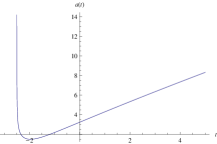
Figure 1: Scale factor $a(t)$ given by (23) for $d_{1}=-2.5$,   $d_{2}=2$ and $d_{3}=1$.

The function $a(t)$ has a vertical asymptote at the point $t=d_{1}$. If $d_{1}<0$ then $a(t)>0$ for all $t>0$. For large values of $t$, $a(t)$ is asymptotically equivalent to $t^{\frac{1}{2}\sqrt{\frac{19}{3}}+\frac{1}{12}\left(3-\sqrt{57}\right)}\approx t^{0.879}$.

$$\ddot{a}(T)=-\frac{d_{3}T^{\frac{1}{12}\left(-21-\sqrt{57}\right)}\left(\left(\sqrt{57}-5\right)d_{2}^{2}T^{2\sqrt{\frac{19}{3}}}-48d_{2}T^{\sqrt{\frac{19}{3}}}-\sqrt{57}-5\right)}{24\left(d_{2}T^{\sqrt{\frac{19}{3}}}+1\right)^{3/2}},$$ (24)

where $T=t-d_{1}$. The expansion is accelerated for $d_{2}(t-d_{1})^{\sqrt{\frac{19}{3}}}<\frac{24}{\sqrt{57}-5}+\frac{4\sqrt{38}}{\sqrt{57}-5}$ and it is decelerated otherwise.

Note that this ansatz $\Box^{n}R=c_{n}R^{n+1}$ for $n=1$ coincides with ansatz $\Box R=q_{\eta}R^{2},$ when $\eta=\frac{-1\pm\sqrt{57}}{8},$ because then one can take $c_{1}=q_{\eta}=\frac{-9\pm\sqrt{57}}{8}.$ In this particular case they have the same scalar curvature $R$ and the same Hubble parameter for $d_{2}=0.$ However, apart from this special case $\eta=\frac{-1\pm\sqrt{57}}{8},$ constant $q_{\eta}$ is different of $c_{1}=\frac{-9\pm\sqrt{57}}{8}.$

Case $\alpha=\frac{1}{2}$.   Putting $\alpha=\frac{1}{2}$ into equation (20) we obtain

$$R(t)=\frac{256}{\left(t+d_{1}\right){}^{4}}.$$ (25)

From (6) we obtain

$$H(t)=\frac{-512\sqrt{3}d_{2}e^{\frac{32}{\sqrt{3}\left(d_{1}+t\right)}}+3(t+d_{1})\left(32d_{2}e^{\frac{32}{\sqrt{3}\left(d_{1}+t\right)}}+\sqrt{3}\right)+48}{6\left(d_{1}+t\right){}^{2}\left(32d_{2}e^{\frac{32}{\sqrt{3}\left(d_{1}+t\right)}}+\sqrt{3}\right)}$$ (26)

and then

$$a(t)=d_{3}e^{-\frac{8}{\sqrt{3}\left(d_{1}+t\right)}}\sqrt{d_{1}+t}\sqrt{32d_{2}e^{\frac{32}{\sqrt{3}\left(d_{1}+t\right)}}+\sqrt{3}},$$ (27)

where $d_{1},\,d_{2},\,d_{3}$ are some real constants.

.

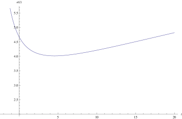
Figure 2: Scale factor $a(t)$ given by (27) for $d_{1}=\frac{8}{\sqrt{3}}$, $d_{2}=2$ and $d_{3}=\frac{1}{10}$.

The corresponding acceleration is

$$\ddot{a}(t) =\frac{d_{3}e^{-\frac{8}{\sqrt{3}\left(d_{1}+t\right)}}}{12\left(d_{1}+t\right){}^{7/2}\left(32d_{2}e^{\frac{32}{\sqrt{3}\left(d_{1}+t\right)}}+\sqrt{3}\right){}^{3/2}}\Big{(}1024\,d_{2}^{2}\,e^{\frac{64}{\sqrt{3}\left(c_{1}+t\right)}}$$

$$\times\left(-6d_{1}t-3d_{1}^{2}+32\sqrt{3}d_{1}-3t^{2}+32\sqrt{3}t+256\right)$$

$$-3\left(6d_{1}t+3d_{1}^{2}+32\sqrt{3}d_{1}+3t^{2}+32\sqrt{3}t-256\right)$$

$$-192\sqrt{3}d_{2}e^{\frac{32}{\sqrt{3}\left(d_{1}+t\right)}}\left(d_{1}+t-16\right)\left(d_{1}+t+16\right)\Big{)}.$$ (28)

The acceleration is positive for $t<t_{0}$ and negative for $t>t_{0},$ where $t_{0}$ is the zero of $\ddot{a}(t).$ For large values of $t$, $\ddot{a}(t)$ converges to 0.

Case $\alpha=2$.   In the case $\alpha=2$ only one integration can be performed and it gives

$$H(t)=\frac{-\sqrt{3}d_{2}I_{1}\left(\frac{2\sqrt{t-d_{1}}}{\sqrt{3}}\right)-d_{2}\sqrt{t-d_{1}}I_{0}\left(\frac{2\sqrt{t-d_{1}}}{\sqrt{3}}\right)-d_{2}\sqrt{t-d_{1}}I_{2}\left(\frac{2\sqrt{t-d_{1}}}{\sqrt{3}}\right)}{4\sqrt{3}\left(t-d_{1}\right)\left(K_{1}\left(\frac{2\sqrt{t-d_{1}}}{\sqrt{3}}\right)-d_{2}I_{1}\left(\frac{2\sqrt{t-d_{1}}}{\sqrt{3}}\right)\right)}$$

$$+\frac{-\sqrt{t-d_{1}}K_{0}\left(\frac{2\sqrt{t-d_{1}}}{\sqrt{3}}\right)+\sqrt{3}K_{1}\left(\frac{2\sqrt{t-d_{1}}}{\sqrt{3}}\right)-\sqrt{t-d_{1}}K_{2}\left(\frac{2\sqrt{t-d_{1}}}{\sqrt{3}}\right)}{4\sqrt{3}\left(t-d_{1}\right)\left(K_{1}\left(\frac{2\sqrt{t-d_{1}}}{\sqrt{3}}\right)-d_{2}I_{1}\left(\frac{2\sqrt{t-d_{1}}}{\sqrt{3}}\right)\right)}.$$ (29)

$I_{i}$ and $K_{i}$ are modified Bessel functions of the first and the second kind, respectively, and $d_{1}$, $d_{2}$ are real constants.

Case $\alpha=-2$.   For $\alpha=-2$ we obtain expression for $H(t)$ involving Airy functions

$$H(t)=\frac{\sqrt[3]{-\frac{1}{3}}\left(d_{2}\text{Ai}^{\prime}\left(\sqrt[3]{-\frac{1}{3}}\left(t-d_{1}\right)\right)+\text{Bi}^{\prime}\left(\sqrt[3]{-\frac{1}{3}}\left(t-d_{1}\right)\right)\right)}{2\left(d_{2}\text{Ai}\left(\sqrt[3]{-\frac{1}{3}}\left(t-d_{1}\right)\right)+\text{Bi}\left(\sqrt[3]{-\frac{1}{3}}\left(t-d_{1}\right)\right)\right)}.$$ (30)

3 Concluding Remarks

In this article we presented three ansätze, two of them are quite new and one can be adjusted so that $\Box^{n}R=0$. These two ansätze have solutions for scalar curvature of the form $R=\frac{C_{2}}{(t+C_{1})^{2}}$, which satisfy all but extended Einstein equations (2) and related trace formula (3). It is a consequence of the quadratic form in $R$ of the Lagrangian (1). However these ansätze are promising for some new nonlocal Lagrangians, which investigation is in progress.

It is worth mentioning that all the above ansätze contain solution $R=0$, which satisfies all (including (2) and (3)) equations with curvature constant $k=-1.$ Namely, for $R=0,$ Eq. (2) reduces to $G_{\mu\nu}=0$ and it gives

$$\frac{\ddot{a}}{a}=0,\quad\quad\Big{(}\frac{\dot{a}}{a}\Big{)}^{2}+\frac{k}{a^{2}}=0.$$ (31)

If $k=0$ one has only static solution $a=constant.$ However, when $k=-1$ then $a(t)=|t|$ and it contains a crunch preceding to a big bang.

Above considered ansätze may be also useful in analysis of some other nonlocal gravity and cosmology models. Further investigation of nonlocality governed by the Riemann zeta function in $p$-adic strings dynamics [14] extends interesting cases and can give new insights.

References

• [1] T. Clifton, P. G. Ferreira, A. Padilla, C. Skordis, “Modified gravity and cosmology”, [arXiv:1106.2476v2 [astro-ph.CO]].
• [2] L. Modesto, “ Super-renormalizable quantum gravity”, [arXiv:1107.2403v1 [hep-th]].
• [3] T. P. Sotiriou, V. Faraoni, “f(R)𝑓𝑅f(R) theories of gravity”, Rev. Mod. Phys. 82 (2010) 451–497 [arXiv:0805.1726v4 [gr-qc]].
• [4] S. Nojiri, S. D. Odintsov, “Unified cosmic history in modified gravity: from F(R)𝐹𝑅F(R) theory to Lorentz non-invariant models”, Phys. Rept. 505 (2011) 59–144 [arXiv:1011.0544v4 [gr-qc]].
• [5] T. Biswas, T. Koivisto, A. Mazumdar, “Towards a resolution of the cosmological singularity in non-local higher derivative theories of gravity”, JCAP 1011 (2010) 008 [arXiv:1005.0590v2 [hep-th]].
• [6] I. Ya. Aref’eva, L. V. Joukovskaya, S. Yu. Vernov, “Bouncing and accelerating solutions in nonlocal stringy models”, JHEP 0707 (2007) 087 [hep-th/0701184].
• [7] G. Calcagni, M. Montobbio, G. Nardelli, “A route to nonlocal cosmology”, Phys. Rev. D 76 (2007) 126001 [arXiv:0705.3043v3 [hep-th]].
• [8] N. Barnaby, T. Biswas, J. M. Cline, “p𝑝p-Adic inflation”, JHEP 0704 (2007) 056 [hep-th/0612230].
• [9] A. S. Koshelev and S. Yu. Vernov, Analysis of scalar perturbations in cosmological models with a non-local scalar field”, Class. Quant. Grav. 28 (2011) 085019 [arXiv:1009.0746v2 [hep-th]].
• [10] G. Calcagni and G. Nardelli, “Nonlocal gravity and the diffusion equation”, Phys. Rev. D 82 (2010) 123518 [arXiv:1004.5144v2 [hep-th]].
• [11] A. S. Koshelev, “Modified non-local gravity”, [arXiv:1112.6410v1 [hep-th]].
• [12] A. S. Koshelev and S. Yu. Vernov, “On bouncing solutions in non-local gravity”, [arXiv:1202.1289v1 [hep-th]].
• [13] T. Biswas, A. Mazumdar and W. Siegel, “Bouncing universes in string-inspired gravity, JCAP 0603 (2006) 009 [arXiv:hep-th/0508194].
• [14] B. Dragovich, “Nonlocal dynamics of p𝑝p-adic strings”, Theor. Math. Phys. 164 (3) (2010) 1151–115 [arXiv:1011.0912v1 [hep-th]].