Stability estimates of nearly–integrable systems with dissipation and non–resonant frequency

Abstract

We consider a dissipative vector field which is represented by a nearly–integrable Hamiltonian flow to which a non symplectic force is added, so that the phase space volume is not preserved. The vector field depends upon two parameters, namely the perturbing and dissipative parameters, and by a drift function. We study the general case of an $\ell$–dimensional, time–dependent vector field. Assuming to start with non–resonant initial conditions, we prove the stability of the variables which are actions of the conservative system (namely, when the dissipative parameter is set to zero) for exponentially long times. In order to construct the normal form, a suitable choice of the drift function must be performed. We also provide some simple examples in which we construct explicitly the normal form, we make a comparison with a numerical integration and we compute theoretical bounds on the parameters as well as we give explicit stability estimates.

                                                 To Professor Anatoly Pavlovich Markeev,

                                                 on the occasion of his 70th birthday

Keywords. Dissipative system, Stability, Non–resonant motion.

1 Introduction

A breakthrough in the theory of the stability of nearly–integrable Hamiltonian systems was achieved by the seminal works of A.N. Kolmogorov ([32]), V.I. Arnold ([1], [2]), J. Moser ([35]) and N.N. Nekhoroshev ([36], [37]). Nearly–integrable systems can be modeled by Hamiltonian functions of the form

$$H(y,x,t)=H_{0}(y)+\varepsilon H_{1}(y,x,t)\ ,$$ (1)

where, for an $\ell$–dimensional system, $y\in{\mathbb{R}}^{\ell}$, $(x,t)\in{\mathbb{T}}^{\ell+1}$, $H_{0}$, $H_{1}$ are regular functions, $H_{1}$ being periodic in $x$ and $t$, and $\varepsilon$ is a small parameter, called the perturbing parameter. As far as $\varepsilon=0$, Hamilton’s equations associated to (1) are integrable. The actions are constants and the motion is described by periodic or quasi–periodic solutions, according to the rational or irrational character of the frequency vector, say $\omega(y)=\partial H_{0}(y)/\partial y$. In this context, under general assumptions, KAM theory yields the persistence of invariant tori for sufficiently small values of the perturbing parameter, which implies a stability property for low–dimensional systems, while higher dimensional models may admit diffusion through the invariant tori. A stability result for arbitrary dimensions can be obtained through Nekhoroshev’s theorem, which guarantees the stability of the actions (namely the confinement in a given domain of the action space) for exponentially long times. Both KAM and Nekhoroshev’s theorems are constructive, in the sense that they can be explicitly implemented to provide bounds on the parameters ensuring the persistence of invariant tori or the confinement of the actions over exponential times. For this reason the theorems have been widely used to investigate physical systems in different contexts. Most notably, Celestial Mechanics was a spur for the development of analytical results about the stability of nearly–integrable systems. In this field, there exist many applications of KAM theorem (compare with [12] and references therein) and of Nekhoroshev’s theorem (see, e.g., [4], [6], [7], [15], [16], [23] [27], [28], [33]); most of the latter papers deal with the stability of the triangular Lagrangian points. All these results are obtained in a conservative framework. However, as it is well known, many interesting physical systems of Celestial Mechanics are affected by a small dissipation. We quote, for example, the three–body problem with Poynting–Robertson drag ([3], [20]) or the spin–orbit model (compare with [34]) with tidal torque ([12]). These problems can be modeled by a nearly–integrable system to which a small dissipation is added (see, e.g., [9]).

While in the conservative setting we find periodic orbits, invariant tori as well as chaotic motions, in the dissipative context (where the phase space volume is not preserved by time evolution) we speak of periodic attractors, quasi–periodic attractors and strange attractors. Beside the case of contracting and expanding systems, we consider also oscillating systems for which the energy varies periodically around a mean value. Coexisting attractors have been established in, e.g., [25], [12]; periodic attractors are shown to exist within parameter regions known as Arnold’s tongues ([9], see also [14]). Concerning invariant attractors, KAM results (both analytical and numerical) provide their persistence under general assumptions (see [8], [10], [11], [13]); an application of the converse KAM theorem (about the non–existence of quasi–periodic attractors) has been presented in [19].

In this paper we exploit exponential type estimates for nearly–integrable dissipative vector fields, which are defined as follows: we consider a vector field depending on two parameters, say $\varepsilon$ and $\mu$, such that for $\mu=0$ we obtain a Hamiltonian vector field in action–angle variables, say $(y,x)\in{\mathbb{R}}^{\ell}\times{\mathbb{T}}^{\ell}$; we consider the most general case of a vector field depending also periodically on the time $t$. We assume that for $\mu\not=0$ the vector field is not conservative; at the first order in $\mu$ the vector field contains a drift function, say $\eta=\eta(y,x,t)$, which must be suitably chosen in order to meet some compatibility conditions, which allow to construct a proper normal form. In this context we establish stability estimates by proving the confinement of the actions of the integrable approximation within a given domain of the phase space for exponentially long times (see [5], [26] and especially [38] which is at the basis of the present work) in the non–conservative non–integrable system. The proof relies on the construction of a proper normal form, which results from the composition of a conservative transformation (removing the conservative terms to suitable orders in $\varepsilon$) and a dissipative transformation, which acts on the $\mu$–dependent terms. Perturbative methods for vector fields have also been developed in [24] (see also [21], [30], [31]). The case of resonant initial conditions is treated in [17], where one needs to construct a Lyapunov function (i.e. the energy function associated to the conservative system with $\mu=0$), which must be used in order to bound the variation of the normal form coordinates; in order to achieve the result, the resonant case requires to work in the extended phase space and to impose the quasi–convexity assumption, which is not needed in the non–resonant case treated here. The final results are conceptually different, since in the non–resonance case we obtain a stability result valid for exponential times, while in the resonant case of [17] the stability time may vary linearly or exponentially with the parameters, according to the structure of the vector field and to the choice of the resonance condition.

We believe that an explicit construction of the normal form and of the stability result in the non–resonant case is certainly of great interest in view of applications to concrete models. Just to quote a field which is familiar to the authors, a non–resonant application in Celestial Mechanics can be of interest in order to bound the motion of the majority of the main belt asteroids.

In this paper we provide also concrete examples by investigating two model problems: a strictly dissipative vector field and a system with oscillating energy. We test the accuracy of the normal form construction by comparing the analytical expression with a numerical integration (see [18] for a discussions about the integration algorithms in nearly–Hamiltonian systems). Furthermore, we compute concrete estimates on the parameters (namely, the radius of the action domain and the stability time) and we investigate their dependence on quantities like the normal form order, obtaining stability times which grow exponentially with the normalization order.

This paper is organized as follows. In Section 2 we set–up the definitions and notations. In Section 3 we state the normal form Lemma and the main Theorem; the proofs are given in Section 4. An application of the normal form Lemma and the computation of the stability estimates according to the results of the Theorem are given in Section 5 .

2 Set–up: notations and assumptions

We consider the following $\ell$–dimensional, time–dependent vector field

$$\dot{x} = \omega(y)+\varepsilon h_{10,y}(y,x,t)+\mu f_{01}(y,x,t)$$

$$\dot{y} = -\varepsilon h_{10,x}(y,x,t)+\mu\Big{(}g_{01}(y,x,t)-\eta(y,x,t)\Big{)}\ ,$$ (2)

where $y\in A$ with $A$ being an open domain of $\mathbb{R}^{\ell}$, $(x,t)\in{\mathbb{T}}^{\ell+1}$, $\varepsilon\in{\mathbb{R}}_{+}$, $\mu\in{\mathbb{R}}\backslash\{0\}$, $\omega$ and $\eta$ are real–analytic, $\ell$–dimensional vector functions with components $(\omega^{(1)},...,\omega^{(\ell)})$ and $(\eta^{(1)},...,\eta^{(\ell)})$. We assume that $h_{10}$, $f_{01}$, $g_{01}$ are known periodic, real–analytic, $\ell$–dimensional functions defined on $A\times{\mathbb{T}}^{\ell+1}$. In all this paper we adopt the following notations and definitions.

$(i)$ The subscripts $x$, $y$ denote derivatives with respect to $x$, $y$.

$(ii)$ For integers $j$, $m$, the symbol $F_{jm}$ denotes that the function $F_{jm}$ is of order $\varepsilon^{j}\mu^{m}$.

$(iii)$ We say that a function $F$ is of order $k$ in $\varepsilon$ and $\mu$, in symbols $F\in O_{k}(\varepsilon,\mu)$, if its Taylor series expansion in $\varepsilon$, $\mu$ contains only powers of $\varepsilon^{j}\mu^{m}$ with $j+m\geq k$.

$(iv)$ For any integer vector $k=(k_{1},...,k_{\ell})\in{\mathbb{Z}}^{\ell}$ we introduce the norm $|k|\equiv|k_{1}|+...+|k_{\ell}|$.

$(v)$ We denote by a bar the average of a function over the angle variables, while the tilde denotes the oscillatory part; more specifically, we decompose a function $F=F(y,x,t)$ as

$$F(y,x,t)=\bar{F}(y)+\tilde{F}(y,x,t)\ ,$$

where the average $\bar{F}(y)$ is given by

$$\bar{F}(y)\equiv\langle F(y,x,t)\rangle_{x,t}={1\over{(2\pi)^{\ell+1}}}\int_{{\mathbb{T}}^{\ell+1}}F(y,x,t)\ dxdt\ ,$$

while the oscillatory part is defined as $\tilde{F}(y,x,t)\equiv F(y,x,t)-\bar{F}(y)$.

We assume that there exists a subset $D\subseteq A$ such that the vector function $\omega=\omega(y)$ satisfies the following non–resonance condition up to a suitable order $K$ with $K\in{\mathbb{Z}}_{+}$:

$$|\omega(y)\cdot k+m|\geq a\quad{\rm for\ all\ }y\in D\ ,\qquad k\in{\mathbb{Z}}^{\ell}\ ,\quad m\in{\mathbb{Z}}\ ,\quad|k|+|m|\leq K\ ,$$ (3)

where $a$ is a strictly positive real constant and the dot denotes the scalar product.

With reference to (2) we call $\varepsilon$ the perturbing parameter, while we refer to $\mu$ as the dissipative parameter. For $\varepsilon=\mu=0$ the equations (2) are trivially integrated as

$$x(t) = x(0)+\omega(y(0))t$$

$$y(t) = y(0)\ ,$$

where $x(0),y(0)$ are the initial conditions at time $t=0$. For $\varepsilon\not=0$ small and $\mu=0$, the equations (2) reduce to the conservative vector field associated to the nearly–integrable Hamiltonian function

$$H(y,x,t)=h_{00}(y)+\varepsilon h_{10}(y,x,t)\ ,$$

where $h_{00}$ is such that $\omega(y)=h_{00,y}(y)$. For $\mu\not=0$ we assume that the vector field is dissipative for any $y\in A$, $(x,t)\in{\mathbb{T}}^{\ell+1}$, namely there exists a subset of the phase space, which is contracted or expanded asymptotically by time evolution into a compact set ([39]). We also consider systems such that the energy is oscillating around a mean value.

We refer to $\eta=\eta(y,x,t)$ as the drift vector function with components $(\eta^{(1)}(y,x,t),...,\eta^{(\ell)}(y,x,t))$, which can be expanded as

$$\eta^{(k)}(y,x,t)=\sum_{m=0}^{\infty}\sum_{j=0}^{m}\eta_{j,m-j+1}^{(k)}(y,x,t)\varepsilon^{j}\mu^{m-j}\ ,\qquad k=1,...,\ell\ .$$

We remark that $\eta$ is an unknown function, which will be properly chosen in order to meet some compatibility requirements in order to perform a suitable normal form (compare with KAM results like in [11]).

Let a function $f=f(y,x,t)$ be defined for $y\in A$, $(x,t)\in{\mathbb{T}}^{\ell+1}$; we denote by $C_{r_{0}}(A)$ the complex neighborhood of $A$ of radius $r_{0}$, namely

$$C_{r_{0}}(A)\equiv\{{y\in\mathbb{C}^{\ell}:}\ \|y-y_{A}\|\leq r_{0}\ {\rm for\ all\ }y_{A}\in A\}\ ,$$

where $\|\cdot\|$ denotes the Euclidean norm. Let $C_{s_{0}}({\mathbb{T}}^{\ell+1})$ be the complex strip of radius $s_{0}$ around ${\mathbb{T}}^{\ell+1}$, namely

$$C_{s_{0}}({\mathbb{T}}^{\ell+1})\equiv\{(x,t)\in{\mathbb{C}}^{\ell+1}:\ \max_{1\leq j\leq\ell}|\Im(x_{j})|\leq s_{0}\ ,\ |\Im(t)|\leq s_{0}\}\ ,$$

where $\Im$ denotes the imaginary part. Let us denote the Fourier expansion of a function $f=f(y,x,t)$ as

$$f(y,x,t)=\sum_{(k,m)\in{\mathbb{Z}}^{\ell+1}}\hat{f}_{km}(y)e^{i(k\cdot x+mt)}\ .$$

For an analytic function on $A\times{\mathbb{T}}^{\ell+1}$ we introduce the norm

$$\|f\|_{r_{0},s_{0}}\equiv\sup_{y\in C_{r_{0}}(A)}\ \sum_{(k,m)\in{\mathbb{Z}}^{\ell+1}}|\hat{f}_{km}(y)|\,e^{(|k|+|m|)s_{0}}\ ,$$

while for a function $g=g(y)$, $g:{\mathbb{R}}^{\ell}\to\mathbb{R}$, we define $\|g\|_{r_{0}}\equiv\sup_{y\in C_{r_{0}}(A)}\|g(y)\|$. For an $\ell$–dimensional vector function $v$ with components $(v_{1},...,v_{\ell})$, we define

$$\|v\|_{r_{0},s_{0}}\equiv\sqrt{\sum_{j=1}^{\ell}\|v_{j}\|_{r_{0},s_{0}}^{2}}\ .$$

For a function $f=f(y,x,t)$, $f:{\mathbb{R}}^{\ell}\times{\mathbb{T}}^{\ell+1}\to{\mathbb{R}}$, and for any positive integer $K$, we denote by $f^{\leq K}$, $f^{>K}$ the sum over the components with Fourier modes less or equal, or respectively greater than $K$, namely

$$f^{\leq K}(y,x,t)\equiv\sum_{(k,m)\in{\mathbb{Z}}^{\ell+1},\ |k|+|m|\leq K}\hat{f}_{km}(y)e^{i(k\cdot x+mt)}$$

and

$$f^{>K}(y,x,t)\equiv\sum_{(k,m)\in{\mathbb{Z}}^{\ell+1},\ |k|+|m|>K}\hat{f}_{km}(y)e^{i(k\cdot x+mt)}\ .$$

3 Stability for exponential times: statement of the results

Stability estimates for exponential times are obtained by implementing a change of coordinates such that the vector field (2) is transformed to a suitable normal form of order $N$. Precisely, let us consider a coordinate transformation close to the identity, say $\Xi^{(n)}:A\times{\mathbb{T}}^{\ell+1}\to{\mathbb{R}}^{\ell}\times{\mathbb{T}}^{\ell+1}$, such that

$$(Y,X,t)=\Xi^{(N)}(y,x,t)\ ,\qquad Y\in{\mathbb{R}}^{\ell}\ ,\qquad(X,t)\in{\mathbb{T}}^{\ell+1}\ ,$$ (4)

where $\Xi^{(N)}$ depends parametrically also on $\varepsilon$, $\mu$; we require that the transformation acts as the identity on the time. Let us assume that on a suitable parameter domain, the coordinate transformation (4) can be inverted as

$$y=y(Y,X,t),\qquad x=x(Y,X,t)\ .$$

In the following Normal Form Lemma we look for a change of coordinates (4) such that (2) is transformed to the following normal form of order $N$:

$$\dot{X} = \Omega_{d}^{(N)}(Y;\varepsilon,\mu)+F_{N+1}(Y,X,t)+F_{01}^{>K}(Y,X,t)$$

$$+ \varepsilon h^{>K}_{10,y}(y(Y,X,t),x(Y,X,t),t)+\mu f^{>K}_{01}(y(Y,X,t),x(Y,X,t),t)$$

$$\dot{Y} = G_{N+1}(Y,X,t)+G_{01}^{>K}(Y,X,t)$$ (5)

$$- \varepsilon h^{>K}_{10,x}(y(Y,X,t),x(Y,X,t),t)+\mu g^{>K}_{01}(y(Y,X,t),x(Y,X,t),t)\ ,$$

where $F_{N+1}$, $G_{N+1}$ are vector functions of order $O_{N+1}(\varepsilon,\mu)$; $F_{01}^{>K}$, $G_{01}^{>K}$ are functions of order $O_{1}(\varepsilon,\mu)$, depending on $\omega$, $h_{10}$, $f_{01}$, $g_{01}$ and on the normal form transformation; $\Omega_{d}^{(N)}:\mathbb{R}^{\ell}\rightarrow\mathbb{R}^{\ell}$ is an $\ell$–dimensional vector function, related to $\omega(Y)$ by

$$\Omega_{d}^{(N)}(Y;\varepsilon,\mu)\equiv\omega(Y)+\sum_{m=0}^{N}\sum_{j=0}^{m}\Omega_{j,m-j}(Y)\varepsilon^{j}\mu^{m-j}\ ,$$

being $\Omega_{j,m-j}(Y)$ known vector functions and being $\Omega_{00}=0$. The meaning of (3) is that the normalized equations take the following form: the $X$–variation is provided by a modified frequency $\Omega_{d}^{(N)}$ plus higher order terms in the normalization order $N$ or in the non–resonance order $K$; the variation of the normal form variable $Y$ is constant, beside higher order terms in $N$ and $K$.

The coordinate transformation $\Xi^{(N)}$ results from the composition of a transformation $\Xi^{(N)}_{c}$ acting on the conservative part and a change of coordinates $\Xi^{(N)}_{d}$ acting on the dissipative part, say:

$$(Y,X,t)=\Xi^{(N)}_{d}\circ\Xi^{(N)}_{c}(y,x,t)\ .$$ (6)

Setting the intermediate variables as $(\tilde{y},\tilde{x},t)\equiv\Xi^{(N)}_{c}(y,x,t)$, the transformation $\Xi^{(N)}_{c}$ is implicitly defined through a sequence of generating functions $\psi_{j0}=\psi_{j0}(\tilde{y},x,t)$, $j=1,...,N$, as

$$\tilde{x} = x+\sum_{j=1}^{N}\psi_{j0,y}(\tilde{y},x,t)\varepsilon^{j}\equiv x+\psi_{y}^{(N)}(\tilde{y},x,t)$$

$$y = \tilde{y}+\sum_{j=1}^{N}\psi_{j0,x}(\tilde{y},x,t)\varepsilon^{j}\equiv\tilde{y}+\psi_{x}^{(N)}(\tilde{y},x,t)\ ,$$ (7)

while $\Xi^{(N)}_{d}$ is defined by introducing suitable functions $\alpha_{jm}$, $\beta_{jm}$, $j,m\in{\mathbb{Z}}_{+}$, as

$$X = \tilde{x}+\sum_{m=0}^{N}\sum_{j=0}^{m}\alpha_{j,m-j}(\tilde{y},\tilde{x},t)\varepsilon^{j}\mu^{m-j}$$

$$Y = \tilde{y}+\sum_{m=0}^{N}\sum_{j=0}^{m}\beta_{j,m-j}(\tilde{y},\tilde{x},t)\varepsilon^{j}\mu^{m-j}\ ,$$ (8)

with the properties that $\alpha_{i0}(\tilde{y},\tilde{x},t)=\beta_{i0}(\tilde{y},\tilde{x},t)=0$ for any $i\geq 0$ and $\langle\alpha_{ij}(\tilde{y},\tilde{x},t)\rangle_{\tilde{x},t}=\langle\beta_{ij}(\tilde{y},\tilde{x},t)\rangle_{\tilde{x},t}=0$. The proof of the following lemma provides an algorithm to compute explicitly the vector functions $\psi_{j0}$, $\alpha_{jm}$, $\beta_{jm}$, together with a suitable drift function $\eta$, which allows to achieve the desired normal form.

Normal Form Lemma. Consider the real analytic vector field (2) defined on $A\times{\mathbb{T}}^{\ell+1}$ with complex extension in $C_{r_{0}}(A)\times C_{s_{0}}({\mathbb{T}}^{\ell+1})$ for some $r_{0}$, $s_{0}>0$. Let $D\subseteq A$ be such that for any $y\in D$, the frequency $\omega=\omega(y)$ satisfies (3) for some $K\in{\mathbb{Z}}_{+}$, $a>0$. Then, there exist $\varepsilon_{0}$, $\mu_{0}>0$ depending on $r_{0}$, $s_{0}$, $K$ and the norms of $\omega$, $h$, $f$, $g$ and there exists $\eta=\eta(y,x,t)$, such that for $(\varepsilon,|\mu|)\leq(\varepsilon_{0},\mu_{0})$, one can find a coordinate transformation close to the identity, say $\Xi^{(N)}:A\times{\mathbb{T}}^{\ell+1}\to{\mathbb{R}}^{\ell}\times{\mathbb{T}}^{\ell+1}$ for a suitable normalization order $N\in\mathbb{Z}_{+}$, which brings (2) into a normal form of order $N$ as in (3). For $\tilde{r}_{0}<r_{0}$, the normalized frequency $\Omega_{d}^{(N)}$ in (3) is bounded by

$$\|\Omega_{d}^{(N)}-\omega\|_{\tilde{r}_{0}}\leq C_{\omega}\lambda\ ,$$

where $\lambda\equiv\max(\varepsilon,|\mu|)$ and $C_{\omega}$ is a suitable positive constant depending on $r_{0}$, $N$ and on the norms of $\omega$, $h$, $f$, $g$, respectively. Let $R_{0}<r_{0}$, $S_{0}<s_{0}$; with reference to the normal form equations (3), the following estimate holds:

$$\|G_{N+1}\|_{R_{0},S_{0}}+\|G^{>K}_{01}\|_{R_{0},S_{0}}+\varepsilon\|h^{>K}_{10,x}\|_{R_{0},S_{0}}+|\mu|\|g^{>K}_{01}\|_{R_{0},S_{0}}\leq C_{Y}\lambda^{N+1}\ ,$$ (9)

for some positive constant $C_{Y}$ depending on $r_{0}$, $s_{0}$, $N$, $K$ and the norms of $\omega$, $h$, $f$, $g$. Choosing $N=[K\tau_{0}/|\log\lambda|]$ for some $\tau_{0}>0$, one gets that (9) becomes

$$\|G_{N+1}\|_{R_{0},S_{0}}+\|G^{>K}_{01}\|_{R_{0},S_{0}}+\varepsilon\|h^{>K}_{10,x}\|_{R_{0},S_{0}}+|\mu|\|g^{>K}_{01}\|_{R_{0},S_{0}}\leq C_{Y}\lambda e^{-K\tau_{0}}\ .$$

Finally, denoting by $\Pi_{y}$ the projection on the $y$–coordinate, one has

$$\|\Pi_{y}(\Xi_{d}^{(N)}\circ\Xi_{c}^{(N)})-Id\|\leq C_{p}\lambda\ ,$$ (10)

for some constant $C_{p}>0$ depending on $r_{0}$, $s_{0}$, $N$ and on the norm of $\omega$, $h$, $f$ and $g$.

Remark. As an outcome of the proof of the Normal Form Lemma, the drift $\eta$ will depend only on the normal form variable $Y$, i.e. $\eta=\eta(Y)$. The explicit form of $\eta$ depends upon the functions $h_{10}$, $f_{01}$, $g_{01}$ appearing in (2); we remark that the value of $\eta$ is determined by the requirement that $Y$ is constant up to the normalization order $N$, say $Y=Y_{0}+O_{N+1}(\varepsilon,\mu)$; on the other hand, $Y_{0}$ depends on $y_{0}$, which is chosen so that the frequency $\omega=\omega(y)$ satisfies (3). The fact that $\eta$ is linked to the form of the vector field and to the frequency of motion appears also in KAM proofs for dissipative (or conformally symplectic) systems (compare with [13], [11]).

Before giving the proof of the Lemma, we provide the statement of the main result, namely the confinement of the $y$ variables for exponential times, which will be obtained through the Normal Form Lemma under the non–resonance condition (3).

Theorem. Consider the vector field (2) defined on $A\times{\mathbb{T}}^{\ell+1}$, and let $D\subseteq A$ be such that for any $y\in D$ the frequency $\omega=\omega(y)$ satisfies (3). Assume there exists $\varepsilon_{0}$, $\mu_{0}$ such that for $(\varepsilon,|\mu|)\leq(\varepsilon_{0},\mu_{0})$ the Normal Form Lemma holds. Then, there exist positive parameters $\rho_{0},\tau_{0}>0$, such that for every solution $(y(t),x(t))$ at time $t>0$ with initial position $(y(0),x(0))\in D\times{\mathbb{T}}^{\ell}$ one has for $\lambda\equiv\max(\varepsilon,|\mu|)$:

$$\|y(t)-y(0)\|\leq\rho_{0}\lambda\quad{for}\quad t\leq C_{t}e^{K\tau_{0}}\ ,$$

for some positive constant $C_{t}$, where $\rho_{0}$ and $C_{t}$ depend on $r_{0}$, $s_{0}$, $N$, $K$, $\varepsilon_{0}$, $\mu_{0}$ and on the norms of $\omega$, $h$, $f$, $g$.

Remark. Notice that we obtain the standard formulation of the stability time in terms of an exponential estimate in the inverse of the small parameters, by adopting a proper choice of $K\tau_{0}$, say $K\tau_{0}\leq({1\over\lambda})^{c}$ for some constant $c>0$; in this case one has that the stability time estimate is $t\leq C_{t}\,e^{{1\over\lambda_{0}^{c}}\,({\lambda_{0}\over\lambda})^{c}}$ for $\lambda_{0}\equiv\max(\varepsilon_{0},\mu_{0})$.

4 Proof of the Normal Form Lemma and of the Theorem

In this section we first outline the general scheme of the proof and then we provide the complete proof of the Normal Form Lemma, followed by that of the main Theorem. For easiness of readability technical Lemmas appear in the Appendixes. We start by implementing a coordinate change of variables of the form (6). In particular, we define the intermediate variables $(\tilde{y},\tilde{x},t)\in\mathbb{R}^{\ell}\times$ ${{\mathbb{T}}^{\ell+1}}$, which provide the transformation (3) in order that the following conservative normal form is obtained:

$$\dot{\tilde{x}} = \Omega_{c}^{(N)}(\tilde{y};\varepsilon)+\mu\sum_{j=1}^{N}F_{j1}^{(1,N)}(\tilde{y},\tilde{x},t)\varepsilon^{j}+\sum_{j=1}^{N}F_{j0}^{(1,N,>K)}(\tilde{y},\tilde{x},t)\varepsilon^{j}$$

$$+ \varepsilon h^{>K}_{10,y}(y(\tilde{y},\tilde{x},t),x(\tilde{y},\tilde{x},t),t)+\mu f^{>K}_{01}(y(\tilde{y},\tilde{x},t),x(\tilde{y},\tilde{x},t),t)+O_{N+1}(\varepsilon,\mu)$$

$$\dot{\tilde{y}} = \mu F^{(2,N)}(\tilde{y},\tilde{x},t)-\mu\left(\eta_{N-1,1}(\tilde{y},\tilde{x},t)\varepsilon^{N-1}+...+\eta_{0N}(\tilde{y},\tilde{x},t)\mu^{N-1}\right)$$ (11)

$$- \varepsilon h^{>K}_{10,x}(y(\tilde{y},\tilde{x},t),x(\tilde{y},\tilde{x},t),t)+\mu g^{>K}_{01}(y(\tilde{y},\tilde{x},t),x(\tilde{y},\tilde{x},t),t)$$

$$+ \sum_{j=1}^{N}F_{j0}^{(3,N,>K)}(\tilde{y},\tilde{x},t)\varepsilon^{j}+O_{N+1}(\varepsilon,\mu)\ ,$$

for suitable functions $F_{j1}^{(1,N)}$, $F_{j0}^{(1,N,>K)}$, $F^{(2,N)}$, $F_{j0}^{(3,N,>K)}$, and being $\Omega_{c}^{(N)}(\tilde{y};\varepsilon)\equiv\omega(\tilde{y})+\sum_{j=1}^{N}\Omega_{j0}(\tilde{y})\varepsilon^{j}$, where $\Omega_{j0}(\tilde{y})$ can be explicitly determined. We denote the inversion of (3) as

$$x = x(\tilde{y},\tilde{x},t)=\tilde{x}+\Gamma^{(x,N)}(\tilde{y},\tilde{x},t)$$

$$y = y(\tilde{y},\tilde{x},t)=\tilde{y}+\Gamma^{(y,N)}(\tilde{y},\tilde{x},t)\ ,$$ (12)

which provides the transformation $\Xi_{c}^{(N)}$. We will see that the generating function $\psi_{j0}(\tilde{y},\tilde{x},t)$ in (3) at the generic order $j$ is the solution of an equation of the following form, defined in terms of the intermediate set of variables:

$$\omega(\tilde{y})\ \psi_{j0,x}(\tilde{y},\tilde{x},t)+\psi_{j0,t}(\tilde{y},\tilde{x},t)+\tilde{L}^{(j,\leq K)}(\tilde{y},\tilde{x},t)=0\ ,$$

for a suitable known function $\tilde{L}^{(j,\leq K)}(\tilde{y},\tilde{x},t)$ with zero average over $(\tilde{x},t)$. The above equation can be solved provided $\omega=\omega(\tilde{y})$ satisfies a non–resonance condition of the form

$$k\cdot\omega(\tilde{y})+m\not=0\qquad{\rm for\ all}\ k\in{\mathbb{Z}}^{\ell}\ ,\ \ m\in{\mathbb{Z}}\ ,\ |k|+|m|\leq K\ ,$$

which is guaranteed by (3) on a suitable domain.

After the implementation of the conservative transformation, to achieve the normal form (3) we construct a change of coordinates $(Y,X,t)=\Xi_{d}^{(N)}(\tilde{y},\tilde{x},t)$ defined as in (3), which allows to obtain the normal form (3). We will see that the functions $\beta_{jm}$ must satisfy an equation of the form

$$\omega(Y)\beta_{jm,x}(Y,X,t)+\beta_{jm,t}(Y,X,t)+N_{jm}^{\leq K}(Y,X,t)-\eta_{jm}(Y,X,t)=0\ ,$$ (13)

for some known function $N_{jm}(Y,X,t)$; therefore, equation (13) can be solved provided that the drift components $\eta_{jm}(Y)$ are chosen as the averages $\bar{N}_{jm}$ of $N_{jm}^{\leq K}$:

$$\eta_{jm}(Y,X,t)\equiv\eta_{jm}(Y)=\bar{N}_{jm}(Y)\ .$$

The normal form equation (13) can be solved provided that the frequency satisfies the non–resonance condition $k\cdot\omega(Y)+m\not=0$ for all $k\in{\mathbb{Z}}^{\ell}$, $m\in{\mathbb{Z}}$, $|k|+|m|\leq K$, which is guaranteed by (3) on a suitable domain. Once $\beta_{jm}$ is determined, we can proceed to compute $\alpha_{jm}$ by solving a normal form equation again of the form (13), but having zero average.

Proof of the Normal Form Lemma. We prove by induction on the normal form order that we can determine the transformations (3) and (3) so to obtain the normal form (3). We start by constructing the first order normal form through the implementation of the conservative and then of the dissipative transformation; in a similar way we construct the transformations for the order $N$. Being the proof quite long, for sake of exposition we split it into separate steps.

Step 1: Conservative transformation for $N=1$.

Let us start with the conservative transformation for $N=1$, namely we implement the first order change of variables

$$\tilde{x} = x+\varepsilon\psi_{10,y}(\tilde{y},x,t)$$

$$y = \tilde{y}+\varepsilon\psi_{10,x}(\tilde{y},x,t)\ ,$$ (14)

where $\psi_{10}=\psi_{10}(\tilde{y},x,t)$ must be determined. Let $\tilde{r}_{0}<r_{0}$, $\delta_{0}<s_{0}$, $\tilde{s}_{0}\equiv s_{0}-\delta_{0}$; then (4) can be inverted as

$$x = \tilde{x}+\varepsilon\Gamma^{(x,1)}(\tilde{y},\tilde{x},t)$$

$$y = \tilde{y}+\varepsilon\Gamma^{(y,1)}(\tilde{y},\tilde{x},t)\ ,$$

for suitable functions $\Gamma^{(x,1)}$ and $\Gamma^{(y,1)}$, provided the following condition is satisfied (see Appendix A):

$$70\,\varepsilon\ \|\psi_{10,y}\|_{\tilde{r}_{0},s_{0}}\ e^{2s_{0}}\delta_{0}^{-1}<1\ .$$ (15)

Using (4) and (2), we compute the time derivatives of $\tilde{x}$, $\tilde{y}$ as

$$\dot{\tilde{x}} = \omega(\tilde{y})+\varepsilon\omega_{y}(\tilde{y})\psi_{10,x}(\tilde{y},\tilde{x},t)+\varepsilon\tilde{h}_{10,y}(\tilde{y},\tilde{x},t)+\varepsilon\bar{h}_{10,y}(\tilde{y})+\mu f_{01}(\tilde{y},\tilde{x},t)$$

$$+ \varepsilon\omega(\tilde{y})\psi_{10,yx}(\tilde{y},\tilde{x},t)+\varepsilon\psi_{10,yt}(\tilde{y},\tilde{x},t)+O_{2}(\varepsilon,\mu)$$

$$\dot{\tilde{y}} = -\varepsilon\tilde{h}_{10,x}(\tilde{y},\tilde{x},t)+\mu\Big{(}g_{01}(\tilde{y},\tilde{x},t)-\eta_{01}(\tilde{y},\tilde{x},t)\Big{)}-\varepsilon\omega(\tilde{y})\psi_{10,xx}(\tilde{y},\tilde{x},t)$$ (16)

$$- \varepsilon\psi_{10,xt}(\tilde{y},\tilde{x},t)+O_{2}(\varepsilon,\mu)\ .$$

The conservative normal form is obtained by imposing that $\psi_{10}(\tilde{y},\tilde{x},t)$ satisfies the following normal form equations:

$$\omega_{y}(\tilde{y})\psi_{10,x}(\tilde{y},\tilde{x},t)+\psi_{10,yt}(\tilde{y},\tilde{x},t)+\omega(\tilde{y})\psi_{10,yx}(\tilde{y},\tilde{x},t)+\tilde{h}^{\leq K}_{10,y}(\tilde{y},\tilde{x},t) = 0$$

$$\omega(\tilde{y})\psi_{10,xx}(\tilde{y},\tilde{x},t)+\psi_{10,xt}(\tilde{y},\tilde{x},t)+\tilde{h}^{\leq K}_{10,x}(\tilde{y},\tilde{x},t) = 0\ .$$ (17)

As a consequence, setting

$$\Omega_{c}^{(1)}(\tilde{y};\varepsilon)\equiv\omega(\tilde{y})+\varepsilon\bar{h}_{10,y}(\tilde{y})\ ,$$ (18)

equations (4) become

$$\dot{\tilde{x}} = \Omega_{c}^{(1)}(\tilde{y};\varepsilon)+\varepsilon h^{>K}_{10,y}(\tilde{y},\tilde{x},t)+\mu f_{01}(\tilde{y},\tilde{x},t)+O_{2}(\varepsilon,\mu)$$

$$\dot{\tilde{y}} = -\varepsilon h^{>K}_{10,x}(\tilde{y},\tilde{x},t)+\mu\Big{(}g_{01}(\tilde{y},\tilde{x},t)-\eta_{01}(\tilde{y},\tilde{x},t)\Big{)}+O_{2}(\varepsilon,\mu)\ ,$$ (19)

which are recognized as being of the form (4). We remark that equations (4) are obtained taking, respectively, the derivatives with respect to $y$ and $x$ of

$$\omega(\tilde{y})\psi_{10,x}(\tilde{y},\tilde{x},t)+\psi_{10,t}(\tilde{y},\tilde{x},t)+\tilde{h}^{\leq K}_{10}(\tilde{y},\tilde{x},t)=0\ .$$

Expanding $\tilde{h}^{\leq K}_{10}(\tilde{y},\tilde{x},t)$ in Fourier series as

$$\tilde{h}^{\leq K}_{10}(\tilde{y},\tilde{x},t)=\sum_{(k,m)\in{\mathbb{Z}}^{\ell+1},|k|+|m|\leq K}{\hat{\tilde{h}}_{10,km}(\tilde{y})}e^{i(k\cdot\tilde{x}+mt)}\ ,$$

where ${\hat{\tilde{h}}_{10,km}(\tilde{y})}$ denote the Fourier coefficients, the solution for $\psi_{10}(\tilde{y},\tilde{x},t)$ is given by:

$$\psi_{10}(\tilde{y},\tilde{x},t)=i\sum_{(k,m)\in{\mathbb{Z}}^{\ell+1},|k|+|m|\leq K}{{\hat{\tilde{h}}_{10,km}(\tilde{y})}\over{\omega(\tilde{y})\cdot k+m}}\ e^{i(k\cdot\tilde{x}+mt)}\ .$$

To control the small divisors appearing in the previous expression, let us invert the second in (4) as $\tilde{y}=y+\varepsilon R^{(1)}(y,x,t)$ for a suitable function $R^{(1)}=R^{(1)}(y,x,t)$, provided that for $\tilde{r}_{0}^{\prime}<r_{0}$ one has (compare with Appendix A)

$$70\,\varepsilon\|\psi_{10,x}\|_{\tilde{r}_{0},s_{0}}{1\over{\tilde{r}_{0}-\tilde{r}_{0}^{\prime}}}<1\ .$$ (20)

Then, we have that

$$|\omega(\tilde{y})\cdot k+m|\geq a-\varepsilon K\|R^{(1)}\|_{\tilde{r}_{0}^{\prime},s_{0}}\|\omega_{y}\|_{r_{0}}\geq{a\over 2}\ ,$$

if (compare with Appendix A)

$$\varepsilon\leq{a\over{2K\|R^{(1)}\|_{\tilde{r}_{0}^{\prime},s_{0}}\|\omega_{y}\|_{r_{0}}}}\ .$$ (21)

Step 2: Dissipative transformation for $N=1$.

We proceed to reduce to normal form the dissipative part through a first–order transformation of coordinates $\Delta_{d}^{(1)}$, which we write in components as

$$X = \tilde{x}+\alpha_{01}(\tilde{y},\tilde{x},t)\mu$$

$$Y = \tilde{y}+\beta_{01}(\tilde{y},\tilde{x},t)\mu\ ,$$ (22)

for some functions $\alpha_{01}$ and $\beta_{01}$ to be determined as follows. We premise that equations (4) can be inverted as

$$\tilde{x} = X+\Delta^{(x,1)}(Y,X,t)\mu$$

$$\tilde{y} = Y+\Delta^{(y,1)}(Y,X,t)\mu$$

for suitable functions $\Delta^{(x,1)}$ and $\Delta^{(y,1)}$ provided the following conditions are satisfied (see Appendix A):

$$70\,|\mu|\ \|\alpha_{01}\|_{\tilde{r}_{0},\tilde{s}_{0}}\ e^{2\tilde{s}_{0}}\tilde{\delta}_{0}^{-1}<1$$

$$70\,|\mu|\ (\|\beta_{01}\|_{\tilde{r}_{0},\tilde{s}_{0}}+|\mu|\|\beta_{01,x}\|_{\tilde{r}_{0},\tilde{s}_{0}}\ \|\alpha_{01}\|_{\tilde{r}_{0},\tilde{s}_{0}})\ {1\over{\tilde{r}_{0}-R_{0}}}<1\ ,$$ (23)

where $\tilde{\delta}_{0}\equiv\tilde{s}_{0}/2$, $R_{0}<\tilde{r}_{0}$ and being $\|\Delta^{(x,1)}\|_{R_{0},S_{0}}\leq\|\alpha_{01}\|_{\tilde{r}_{0},\tilde{s}_{0}}$ with $S_{0}<\tilde{s}_{0}-\tilde{\delta}_{0}$. Up to the second order, the inversion of (4) provides

$$\tilde{x} = X-\alpha_{01}(Y,X,t)\mu+O_{2}(\mu)$$

$$\tilde{y} = Y-\beta_{01}(Y,X,t)\mu+O_{2}(\mu)\ .$$ (24)

Taking the derivative of (4) and using (4), we express $\dot{X}$, $\dot{Y}$ as a function of $X$, $Y$ as

$$\dot{X} = \omega(Y)-\omega_{y}(Y)\beta_{01}(Y,X,t)\mu+\varepsilon{\bar{h}}_{10,y}(Y)$$

$$+ \varepsilon{h}^{>K}_{10,y}(Y,X,t)+\mu f_{01}(Y,X,t)+\omega(Y)\alpha_{01,x}(Y,X,t)\mu$$

$$+ \alpha_{01,t}(Y,X,t)\mu+O_{2}(\varepsilon,\mu)$$

$$\dot{Y} = -\varepsilon{h}^{>K}_{10,x}(Y,X,t)+\mu\Big{(}g_{01}(Y,X,t)-\eta_{01}(Y,X,t)\Big{)}$$

$$+ \omega(Y)\beta_{01,x}(Y,X,t)\mu+\beta_{01,t}(Y,X,t)\mu+O_{2}(\varepsilon,\mu)\ .$$

The dissipative normal form is obtained imposing that $\alpha_{01}$, $\beta_{01}$ and $\eta_{01}$ satisfy the following equations:

$$\omega(Y)\alpha_{01,x}(Y,X,t)+\alpha_{01,t}(Y,X,t)-\omega_{y}(Y)\beta_{01}(Y,X,t)+\tilde{f}_{01}^{\leq K}(Y,X,t) = 0$$

$$\omega(Y)\beta_{01,x}(Y,X,t)+\beta_{01,t}(Y,X,t)+\tilde{g}^{\leq K}_{01}(Y,X,t)+\bar{g}_{01}(Y)-\eta_{01}(Y) = 0\ ,$$ (25)

where we have split $f_{01}$ into the sum of its average and of the oscillatory part, namely

$$f_{01}(Y,X,t)\equiv\bar{f}_{01}(Y)+\tilde{f}_{01}^{\leq K}(Y,X,t)+f_{01}^{>K}(Y,X,t)$$

and similarly for $g_{01}$: $g_{01}(Y,X,t)\equiv\bar{g}_{01}(Y)+\tilde{g}_{01}^{\leq K}(Y,X,t)+g_{01}^{>K}(Y,X,t)$. From the first of (4) we see that the average of $\beta_{01}$ is zero and we can assume that also the average of $\alpha_{01}$ is zero. Then, equations (4) can be solved, provided that in the second equation the term $\eta_{01}(Y,X,t)$ is chosen so that

$$\eta_{01}(Y,X,t)\equiv\eta_{01}(Y)=\bar{g}_{01}(Y)\ .$$

The final normal form can be written as

$$\dot{X} = \omega(Y)+\varepsilon{\bar{h}}_{10,y}(Y)+\mu\bar{f}_{01}(Y)+\varepsilon h^{>K}_{10,y}(Y,X,t)+\mu f^{>K}_{01}(Y,X,t)+F_{2}(Y,X,t)$$

$$\dot{Y} = -\varepsilon h^{>K}_{10,x}(Y,X,t)+\mu g^{>K}_{01}(Y,X,t)+G_{2}(Y,X,t)\ ,$$

where $F_{2}$, $G_{2}$ are $O_{2}(\varepsilon,\mu)$. These equations are recognized to be of the form (3) with $\Omega_{d}^{(1)}(Y)=\omega(Y)+\varepsilon\bar{h}_{10}(Y)+\mu\bar{f}_{01}(Y)$.

The solutions of (4) involves small divisors, which can be bounded as follows:

$$|\omega(Y)\cdot k+m|\geq{a\over 2}-|\mu|K\|\beta_{01}\|_{\tilde{r}_{0},\tilde{s}_{0}}\|\omega_{y}\|_{r_{0}}>{a\over 4}\ ,$$

provided that (see Appendix A)

$$|\mu|<{a\over{4K\|\beta_{01}\|_{\tilde{r}_{0},\tilde{s}_{0}}\|\omega_{y}\|_{r_{0}}}}\ .$$ (26)

Step 3: Conservative transformation for the order $N$.

Assuming that the Lemma holds up to the order $N-1$, we prove it for the order $N$, starting from the change of variables (3), that we invert as

$$x = \tilde{x}+\sum_{j=1}^{N}\Gamma_{j0}^{(x)}(\tilde{y},\tilde{x},t)\varepsilon^{j}-\psi_{N0,y}(\tilde{y},\tilde{x},t)\varepsilon^{N}+O_{N+1}(\varepsilon)\equiv\tilde{x}+\Gamma^{(x,N)}(\tilde{y},\tilde{x},t)$$

$$y = \tilde{y}+\sum_{j=1}^{N}\Gamma_{j0}^{(y)}(\tilde{y},\tilde{x},t)\varepsilon^{j}+\psi_{N0,x}(\tilde{y},\tilde{x},t)\varepsilon^{N}+O_{N+1}(\varepsilon)\equiv\tilde{y}+\Gamma^{(y,N)}(\tilde{y},\tilde{x},t)\ ,$$ (27)

where $\Gamma_{j0}^{(x)}$, $\Gamma_{j0}^{(y)}$ are known, since they depend on the known functions $\psi_{10}$, …, $\psi_{N-1,0}$, while $\Gamma^{(x,N)}$, $\Gamma^{(y,N)}$ have been introduced as in (4). Choosing $\tilde{r}_{0}<r_{0}$, $\delta_{0}<s_{0}$, the inversion is possible provided that (see Appendix A)

$$70\,\|\psi^{(N)}_{y}\|_{\tilde{r}_{0},s_{0}}\ e^{2s_{0}}\delta_{0}^{-1}\ <\ 1\ ,$$ (28)

being $\psi^{(N)}=\sum_{j=1}^{N}\psi_{j0}\varepsilon^{j}$. For short, let us write the equations (4) as

$$x=x(\tilde{y},\tilde{x},t)\ ,\qquad y=y(\tilde{y},\tilde{x},t)\ .$$

Inserting (4) in (2) and expanding in Taylor series, one has

$$\dot{x} = \omega(\tilde{y})+\omega_{y}(\tilde{y})\psi_{N0,x}(\tilde{y},\tilde{x},t)\varepsilon^{N}+F^{(0,N)}(\tilde{y},\tilde{x},t)$$

$$+ \varepsilon h^{>K}_{10,y}(y(\tilde{y},\tilde{x},t),x(\tilde{y},\tilde{x},t),t)+\mu f^{>K}_{01}(y(\tilde{y},\tilde{x},t),x(\tilde{y},\tilde{x},t),t)+O_{N+1}(\varepsilon,\mu)\noindent$$

$$\dot{y} = G^{(0,N)}(\tilde{y},\tilde{x},t)-\mu\left(\eta_{N-1,1}(\tilde{y},\tilde{x},t)\varepsilon^{N-1}+...+\eta_{0,N}(\tilde{y},\tilde{x},t)\mu^{N-1}\right)$$

$$- \varepsilon h^{>K}_{10,x}(y(\tilde{y},\tilde{x},t),x(\tilde{y},\tilde{x},t),t)+\mu g^{>K}_{01}(y(\tilde{y},\tilde{x},t),x(\tilde{y},\tilde{x},t),t)+O_{N+1}(\varepsilon,\mu)\ ,$$

where $F^{(0,N)}$, $G^{(0,N)}$ are known functions; $F^{(0,N)}$ contains terms of order $\varepsilon$, $\varepsilon^{2}$, …, $\varepsilon^{N}$, $\mu$, $\mu\varepsilon$, …, $\mu\varepsilon^{N-1}$, while $G^{(0,N)}$ contains all powers $\varepsilon^{j}\mu^{m}$ with $1\leq j+m\leq N$. Next step is to compute $\dot{\tilde{x}}$, $\dot{\tilde{y}}$ as a function of $\tilde{x}$, $\tilde{y}$. Taking into account (3) and that by the inductive hypothesis $\psi^{(1)}$, …, $\psi^{(N-1)}$ make the equations in normal form up to the order $N-1$, we obtain

$$\dot{\tilde{x}} = \omega(\tilde{y})+\sum_{j=1}^{N}\bar{F}^{(1,N)}_{j0}(\tilde{y})\varepsilon^{j}+\Big{[}\omega_{y}(\tilde{y})\psi_{N0,x}(\tilde{y},\tilde{x},t)+\omega(\tilde{y})\psi_{N0,yx}(\tilde{y},\tilde{x},t)+\psi_{N0,yt}(\tilde{y},\tilde{x},t)$$

$$+ \tilde{F}^{(1,N,\leq K)}_{N0}(\tilde{y},\tilde{x},t)\Big{]}\varepsilon^{N}+\mu\sum_{j=1}^{N-1}F^{(1,N)}_{j1}(\tilde{y},\tilde{x},t)\varepsilon^{j}+\sum_{j=1}^{N}F_{j0}^{(1,N,>K)}(\tilde{y},\tilde{x},t)\varepsilon^{j}$$

$$+ \varepsilon h^{>K}_{10,y}(y(\tilde{y},\tilde{x},t),x(\tilde{y},\tilde{x},t),t)+\mu f^{>K}_{01}(y(\tilde{y},\tilde{x},t),x(\tilde{y},\tilde{x},t),t)+O_{N+1}(\varepsilon,\mu)\ ,$$

where $F^{(1,N)}(\tilde{y},\tilde{x},t)$ is a known function that has been decomposed as

$$F^{(1,N)}(\tilde{y},\tilde{x},t) \equiv \sum_{j=1}^{N}\bar{F}^{(1,N)}_{j0}(\tilde{y})\varepsilon^{j}+\sum_{j=1}^{N-1}\tilde{F}^{(1,N)}_{j0}(\tilde{y},\tilde{x},t)\varepsilon^{j}+\tilde{F}^{(1,N)}_{N0}(\tilde{y},\tilde{x},t)\varepsilon^{N}$$

$$+ \mu\sum_{j=1}^{N-1}F^{(1,N)}_{j1}(\tilde{y},\tilde{x},t)\varepsilon^{j}\ .$$

In a similar way one obtains

$$\dot{\tilde{y}} = \mu F^{(2,N)}(\tilde{y},\tilde{x},t)+\Big{(}\tilde{F}^{(3,N,\leq K)}_{N0}(\tilde{y},\tilde{x},t)-\omega(\tilde{y})\psi_{N0,xx}(\tilde{y},\tilde{x},t)-\psi_{N0,xt}(\tilde{y},\tilde{x},t)\Big{)}\varepsilon^{N}$$

$$- \mu\left(\eta_{N-1,1}(\tilde{y},\tilde{x},t)\varepsilon^{N-1}+...+\eta_{0,N}(\tilde{y},\tilde{x},t)\mu^{N-1}\right)+\sum_{j=1}^{N}F_{j0}^{(3,N,>K)}(\tilde{y},\tilde{x},t)\varepsilon^{j}$$

$$- \varepsilon h^{>K}_{10,x}(y(\tilde{y},\tilde{x},t),x(\tilde{y},\tilde{x},t),t)+\mu g^{>K}_{01}(y(\tilde{y},\tilde{x},t),x(\tilde{y},\tilde{x},t),t)+O_{N+1}(\varepsilon,\mu)\ ,$$

for known functions $F^{(2,N)}$, $\tilde{F}^{(3,N)}$, the latter having zero average. The conservative normal form is obtained by imposing that $\psi_{N0}$ solves the following normal form equations

$$\omega_{y}(\tilde{y})\psi_{N0,x}(\tilde{y},\tilde{x},t)+\omega(\tilde{y})\psi_{N0,yx}(\tilde{y},\tilde{x},t)+\psi_{N0,yt}(\tilde{y},\tilde{x},t)+\tilde{F}^{(1,N,\leq K)}_{N0}(\tilde{y},\tilde{x},t) = 0$$

$$\omega(\tilde{y})\psi_{N0,xx}(\tilde{y},\tilde{x},t)+\psi_{N0,xt}(\tilde{y},\tilde{x},t)-\tilde{F}^{(3,N,\leq K)}_{N0}(\tilde{y},\tilde{x},t) = 0\ ,$$ (29)

where as before we have split the known function $F_{N0}^{(1,N)}$ into $F_{N0}^{(1,N)}=$ $\bar{F}_{N0}^{(1,N)}+\tilde{F}_{N0}^{(1,N)}$ as well as $\tilde{F}_{N0}^{(1,N)}$ into $\tilde{F}_{N0}^{(1,N)}=\tilde{F}_{N0}^{(1,N,\leq K)}+F_{N0}^{(1,N,>K)}$. Note that in this setting the $N$–th order contribution to the shifted frequency vector is given by $\Omega_{N0}(\tilde{y})\equiv\bar{F}^{(1,N)}_{N0}(\tilde{y})$. Due to the Hamiltonian character which occurs for $\mu=0$, there exists a function $M^{(N,\leq K)}=M^{(N,\leq K)}(\tilde{y},\tilde{x},t)$ with zero average, such that

$${{\partial M^{(N,\leq K)}(\tilde{y},\tilde{x},t)}\over{\partial y}}=\tilde{F}^{(1,N,\leq K)}_{N0}(\tilde{y},\tilde{x},t)\ ,\qquad{{\partial M^{(N,\leq K)}(\tilde{y},\tilde{x},t)}\over{\partial x}}=-\tilde{F}^{(3,N,\leq K)}_{N0}(\tilde{y},\tilde{x},t)\ ,$$

so that (4) are equivalent to solve the equation

$$\omega(\tilde{y})\psi_{N0,x}(\tilde{y},\tilde{x},t)+\psi_{N0,t}(\tilde{y},\tilde{x},t)+M^{(N,\leq K)}(\tilde{y},\tilde{x},t)=0\ .$$ (30)

The solution of (30) provides the function $\psi_{N0}(\tilde{y},\tilde{x},t)$, which produces the conservative normal form:

$$\dot{\tilde{x}} = \Omega_{c}^{(N)}(\tilde{y};\varepsilon)+\mu\sum_{j=1}^{N-1}F_{j1}^{(1,N)}(\tilde{y},\tilde{x},t)\varepsilon^{j}+\sum_{j=1}^{N}F_{j0}^{(1,N,>K)}(\tilde{y},\tilde{x},t)\varepsilon^{j}$$

$$+ \varepsilon h^{>K}_{10,y}(y(\tilde{y},\tilde{x},t),x(\tilde{y},\tilde{x},t),t)+\mu f^{>K}_{01}(y(\tilde{y},\tilde{x},t),x(\tilde{y},\tilde{x},t),t)+O_{N+1}(\varepsilon,\mu)$$

$$\dot{\tilde{y}} = \mu F^{(2,N)}(\tilde{y},\tilde{x},t)-\mu\left(\eta_{N-1,1}(\tilde{y},\tilde{x},t)\varepsilon^{N-1}+...+\eta_{0,N}(\tilde{y},\tilde{x},t)\mu^{N-1}\right)$$ (31)

$$- \varepsilon h^{>K}_{10,x}(y(\tilde{y},\tilde{x},t),x(\tilde{y},\tilde{x},t),t)+\mu g^{>K}_{01}(y(\tilde{y},\tilde{x},t),x(\tilde{y},\tilde{x},t),t)$$

$$+ \sum_{j=1}^{N}F_{j0}^{(3,N,>K)}(\tilde{y},\tilde{x},t)\varepsilon^{j}+O_{N+1}(\varepsilon,\mu)\ ,$$

where

$$\Omega_{c}^{(N)}(\tilde{y};\varepsilon)\equiv\omega(\tilde{y})+\sum_{j=1}^{N}\bar{F}_{j0}^{(1,N)}(\tilde{y})\varepsilon^{j}\ .$$ (32)

Notice that from the definition (32) one obtains an estimate like $\|\Omega_{c}^{(N)}-\omega\|\leq C_{c}\varepsilon$ for a suitable constant $C_{c}$. The solution of (30) involves small divisors of the form $\omega(\tilde{y})\cdot k+m$, for $k\in{\mathbb{Z}}^{\ell}$, $m\in{\mathbb{Z}}$ with $|k|+|m|\leq K$, as it was for the case $N=1$; non–resonance is guaranteed provided that (see Appendix A)

$$\varepsilon\leq{a\over{2K\|R^{(N)}\|_{\tilde{r}_{0}^{\prime},s_{0}}\|\omega_{y}\|_{r_{0}}}}\ ,$$ (33)

where $R^{(N)}$ is the function such that $\tilde{y}=y+\varepsilon R^{(N)}(y,x,t)$ and $\tilde{r}_{0}^{\prime}<\tilde{r}_{0}$.

Step 4: Dissipative transformation for the order $N$.

As for the dissipative part, we consider the transformation (3), that we invert as

$$\tilde{x} = X+\sum_{k=0}^{N}\sum_{j=0}^{N-k}a_{kj}(Y,X,t)\varepsilon^{k}\mu^{j}-\sum_{k=0}^{N-1}\alpha_{k,N-k}(Y,X,t)\varepsilon^{k}\mu^{N-k}+O_{N+1}(\varepsilon,\mu)$$

$$\tilde{y} = Y+\sum_{k=0}^{N}\sum_{j=0}^{N-k}b_{kj}(Y,X,t)\varepsilon^{k}\mu^{j}-\sum_{k=0}^{N-1}\beta_{k,N-k}(Y,X,t)\varepsilon^{k}\mu^{N-k}+O_{N+1}(\varepsilon,\mu)\ ,$$ (34)

for suitable known functions $a_{kj}(Y,X,t)$, $b_{kj}(Y,X,t)$ with $a_{k0}=b_{k0}=0$ for $k=0,...,N$, provided the following conditions are satisfied (see Appendix A):

$$70\,\|\alpha^{(N)}\|_{\tilde{r}_{0},\tilde{s}_{0}}\ e^{2\tilde{s}_{0}}\tilde{\delta}_{0}^{-1} < 1$$

$$70\,\left(\|\beta^{(N)}\|_{\tilde{r}_{0},\tilde{s}_{0}}+\|\beta_{x}^{(N)}\|_{\tilde{r}_{0},\tilde{s}_{0}}\|\alpha^{(N)}\|_{\tilde{r}_{0},\tilde{s}_{0}}\right)\ {1\over{\tilde{r}_{0}-R_{0}}} < 1\ ,$$ (35)

where $\tilde{\delta}_{0}\equiv\tilde{s}_{0}/2$, $R_{0}<\tilde{r}_{0}$. For short let us denote (4) as

$$\tilde{x}=\tilde{x}(Y,X,t)\ ,\qquad\tilde{y}=\tilde{y}(Y,X,t)\ ,$$

while we express the original variables in terms of $(Y,X,t)$ through

$$x = x(\tilde{y}(Y,X,t),\tilde{x}(Y,X,t),t)\equiv X+\Phi^{(x,N)}(Y,X,t)$$

$$y = y(\tilde{y}(Y,X,t),\tilde{x}(Y,X,t),t)\equiv Y+\Phi^{(y,N)}(Y,X,t)\ ,$$

for suitable functions $\Phi^{(x,N)}$, $\Phi^{(y,N)}$, which are $O_{1}(\varepsilon,\mu)$. We need to determine the unknown functions $\alpha_{0,N}$, …, $\alpha_{N-1,1}$, $\beta_{0,N}$, …, $\beta_{N-1,1}$, $\eta_{N-1,1}$, …, $\eta_{0,N}$ as follows. Starting from (4), we compute $\dot{\tilde{x}}$, $\dot{\tilde{y}}$ in terms of $X$, $Y$ and we express $\dot{X}$, $\dot{Y}$ in terms of $X$, $Y$, using (3), (4), (4); by the inductive hypothesis $\alpha_{kj}$, $\beta_{kj}$, $\eta_{j}$ with $0\leq k+j\leq N-1$ are determined so that the equations of motion are in normal form up to the order $\varepsilon^{k}\mu^{j}$ with $0\leq k+j\leq N-1$. This leads to the following equations:

$$\dot{X} = \Omega_{c}^{(N)}(Y)-\omega_{y}(Y)\left(\sum_{j=0}^{N-1}\beta_{j,N-j}(Y,X,t)\varepsilon^{j}\mu^{N-j}\right)+\omega(Y)\sum_{j=0}^{N-1}\alpha_{j,N-j,x}(Y,X,t)\varepsilon^{j}\mu^{N-j}$$

$$+ \sum_{j=0}^{N-1}\alpha_{j,N-j,t}(Y,X,t)\varepsilon^{j}\mu^{N-j}+\mu F^{(4,N)}(Y,X,t)$$

$$+ \sum_{j=1}^{N}F_{j0}^{(1,N,>K)}(\tilde{y}(Y,X,t),\tilde{x}(Y,X,t),t)\varepsilon^{j}$$

$$+ \varepsilon h^{>K}_{10,y}(y(Y,X,t),x(Y,X,t),t)+\mu f^{>K}_{01}(y(Y,X,t),x(Y,X,t),t)+O_{N+1}(\varepsilon,\mu)$$

$$\dot{Y} = -\mu\Big{(}\eta_{N-1,1}(Y,X,t)\varepsilon^{N-1}+...+\eta_{0,N}(Y,X,t)\mu^{N-1}\Big{)}+\omega(Y)\sum_{j=0}^{N-1}\beta_{j,N-j,x}(Y,X,t)\varepsilon^{j}\mu^{N-j}$$

$$+ \sum_{j=0}^{N-1}\beta_{j,N-j,t}(Y,X,t)\varepsilon^{j}\mu^{N-j}+\mu F^{(5,N)}(Y,X,t)$$

$$+ \sum_{j=1}^{N}F_{j0}^{(3,N,>K)}(\tilde{y}(Y,X,t),\tilde{x}(Y,X,t),t)\varepsilon^{j}$$

$$- \varepsilon h^{>K}_{10,x}(y(Y,X,t),x(Y,X,t),t)+\mu g^{>K}_{01}(y(Y,X,t),x(Y,X,t),t)+O_{N+1}(\varepsilon,\mu)\ ,$$

where $F^{(4,N)}(Y,X,t)$, $F^{(5,N)}(Y,X,t)$ are $O(\mu^{N-1},\varepsilon\mu^{N-2},...,\varepsilon^{N-2}\mu,\varepsilon^{N-1})$. Let us decompose $F^{(4,N)}$ as $F^{(4,N)}(Y,X,t)=\bar{F}^{(4,N)}(Y)+\tilde{F}^{(4,N)}(Y,X,t)$. The normal form at the order $N$ is achieved imposing that $\alpha_{kj}$, $\beta_{kj}$, $\eta_{j}$ satisfy the following normal form equations

$$-\omega_{y}(Y)\beta_{j,N-j}(Y,X,t)+\omega(Y)\alpha_{j,N-j,x}(Y,X,t)+\alpha_{j,N-j,t}(Y,X,t)$$

$$\qquad\qquad\qquad\qquad\qquad\qquad\qquad\qquad+\tilde{F}^{(4,N,\leq K)}_{j,N-j}(Y,X,t)=0$$

$$\omega(Y)\beta_{j,N-j,x}(Y,X,t)+\beta_{j,N-j,t}(Y,X,t)+\tilde{F}^{(5,N,\leq K)}_{j,N-j}(Y,X,t)$$

$$\qquad\qquad\qquad\qquad\qquad\qquad\qquad\qquad+\bar{F}_{j,N-j}^{(5,N)}(Y)-\eta_{j,N-j}(Y,X,t)=0$$ (36)

for $0\leq j\leq N-1$, where we have used the expansion

$$\mu F^{(m,N)}(Y,X,t)\equiv\sum_{k=0}^{N-1}\bar{F}^{(m,N)}_{k,N-k}(Y)\varepsilon^{k}\mu^{N-k}+\sum_{k=0}^{N-1}\tilde{F}^{(m,N)}_{k,N-k}(Y,X,t)\varepsilon^{k}\mu^{N-k}\ ,\quad m=4,\ 5$$

and we split $\tilde{F}^{(m,N)}_{k,N-k}=\tilde{F}^{(m,N,\leq K)}_{k,N-k}+F^{(m,N,>K)}_{k,N-k}$. The non–resonance condition for $\omega(Y)$ reads as (see Appendix A):

$$K\|\ \beta^{(N)}\|_{\tilde{r}_{0},\tilde{s}_{0}}\|\omega_{y}\|_{r_{0}}<{a\over 4}\ ,$$ (37)

where, for short, we have written $Y\equiv\tilde{y}+\beta^{(N)}(\tilde{y},\tilde{x},t;\varepsilon,\mu)$. From the second of (4), it is

$$\eta_{j,N-j}(Y,X,t)\equiv\eta_{j,N-j}(Y)=\bar{F}^{(5,N)}_{j,N-j}(Y)\ ,$$

so that the second of (4) can be solved to determine $\beta_{j,N-j}$, while from the first of (4) we obtain $\alpha_{j,N-j}$. Identifying the final normalized frequency $\Omega_{d}$ with $\Omega_{d}^{(N)}(Y;\varepsilon,\mu)\equiv\omega(Y)+\sum_{m=0}^{N}\sum_{j=0}^{m}\Omega_{j,m-j}(Y)\varepsilon^{j}\mu^{m-j}\ ,$ where $\Omega_{00}=0$, $\Omega_{10}=\omega$, $\Omega_{j0}\equiv\bar{F}_{j0}^{(1,N)}(Y)$ and $\Omega_{j,m-j}\equiv\bar{F}^{(4,N)}_{j,m-j}(Y)$, the resulting normal form is given by

$$\dot{X} = \Omega_{d}^{(N)}(Y;\varepsilon,\mu)+F_{N+1}(Y,X,t)+\sum_{j=0}^{N-1}F^{(4,N,>K)}_{j,N-j}(Y,X,t)\varepsilon^{j}\mu^{N-j}$$

$$+ \varepsilon h^{>K}_{10,y}(y(Y,X,t),x(Y,X,t),t)+\mu f^{>K}_{01}(y(Y,X,t),x(Y,X,t),t)$$

$$+ \sum_{j=1}^{N}F^{(1,N,>K)}_{j0}(\tilde{y}(Y,X,t),\tilde{x}(Y,X,t),t)\varepsilon^{j}$$

$$\dot{Y} = G_{N+1}(Y,X,t)+\sum_{j=0}^{N-1}F^{(5,N,>K)}_{j,N-j}(Y,X,t)\varepsilon^{j}\mu^{N-j}$$ (38)

$$- \varepsilon h^{>K}_{10,x}(y(Y,X,t),x(Y,X,t),t)+\mu g^{>K}_{01}(y(Y,X,t),x(Y,X,t),t)$$

$$+ \sum_{j=1}^{N}F^{(3,N,>K)}_{j0}(\tilde{y}(Y,X,t),\tilde{x}(Y,X,t),t)\varepsilon^{j}\ ,$$

where $F_{N+1}$, $G_{N+1}$ are $O_{N+1}(\varepsilon,\mu)$. For short, we define

$$F_{01}^{>K}(Y,X,t) \equiv \sum_{j=0}^{N-1}F^{(4,N,>K)}_{j,N-j}(Y,X,t)\varepsilon^{j}\mu^{N-j}+\sum_{j=1}^{N}F_{j0}^{(1,N,>K)}(\tilde{y}(Y,X,t),\tilde{x}(Y,X,t),t)\varepsilon^{j}$$

$$G_{01}^{>K}(Y,X,t) \equiv \sum_{j=0}^{N-1}F^{(5,N,>K)}_{j,N-j}(Y,X,t)\varepsilon^{j}\mu^{N-j}+\sum_{j=1}^{N}F_{j0}^{(3,N,>K)}(\tilde{y}(Y,X,t),\tilde{x}(Y,X,t),t)\varepsilon^{j}\ ,$$

which makes (4) of the form (3). The estimate (10) follows from the fact that (3) is close to the identity up to terms of order $\varepsilon$, while (3) is close to the identity up to terms of order $\mu$. Notice that the smallness requirements on $\varepsilon$, $\mu$, say $\varepsilon\leq\varepsilon_{0}$, $|\mu|\leq\mu_{0}$, are needed to ensure that the non–resonance condition (see (21), (26), (33), (37)) is satisfied and that the transformations (3), (3) can be inverted (see (15), (20), (4), (28), (4)).

The original variables can be expressed in terms of the intermediate variables by means of (4), provided (28) holds with

$$\|\Gamma^{(x,N)}\|_{\tilde{r}_{0},\tilde{s}_{0}}\leq\|\psi_{y}^{(N)}\|_{\tilde{r}_{0},s_{0}}\ ,$$

being $\tilde{s}_{0}\equiv s_{0}-\delta_{0}$. Moreover, we have

$$\|\Gamma^{(y,N)}\|_{\tilde{r}_{0},\tilde{s}_{0}}\leq\|\psi_{x}^{(N)}\|_{\tilde{r}_{0},s_{0}}+\|\psi_{xx}^{(N)}\|_{\tilde{r}_{0},s_{0}}\|\Gamma^{(x,N)}\|_{\tilde{r}_{0},\tilde{s}_{0}}\ .$$

For the same reason, equations (4) are invertible for $\varepsilon$, $|\mu|$ sufficiently small, since the Jacobian of the transformation is close to the identity; we can write the inverse as

$$\tilde{x} = X+\Delta^{(x,N)}(Y,X,t)$$

$$\tilde{y} = Y+\Delta^{(y,N)}(Y,X,t)$$

for suitable, bounded functions $\Delta^{(x,N)}$, $\Delta^{(y,N)}$ of order $O_{1}(\varepsilon,\mu)$. We finally obtain

$$x = X+\Delta^{(x,N)}(Y,X,t)+\Gamma^{(x,N)}(Y+\Delta^{(y,N)}(Y,X,t),X+\Delta^{(x,N)}(Y,X,t),t)$$

$$\equiv X+\Phi^{(x,N)}(Y,X,t)$$

$$y = Y+\Delta^{(y,N)}(Y,X,t)+\Gamma^{(y,N)}(Y+\Delta^{(y,N)}(Y,X,t),X+\Delta^{(x,N)}(Y,X,t),t)$$

$$\equiv Y+\Phi^{(y,N)}(Y,X,t)\ .$$

Recalling Lemma B.1 of Appendix B, for $\tau_{0}>0$ and $1\leq j\leq\ell$, we have

$$\|h^{>K}_{10,x}\|_{R_{0},S_{0}} \leq C_{a}\|h_{10,x}\|_{R_{0},S_{0}+\tau_{0}}e^{-(K+1)\tau_{0}}$$

$$\|h^{>K}_{10,xy_{j}}\|_{R_{0},S_{0}} \leq C_{a}\|h_{10,xy_{j}}\|_{R_{0},S_{0}+\tau_{0}}e^{-(K+1)\tau_{0}}$$

$$\|h^{>K}_{10,xx_{j}}\|_{R_{0},S_{0}} \leq C_{a}\|h_{10,xx_{j}}\|_{R_{0},S_{0}+\tau_{0}}e^{-(K+1)\tau_{0}}\ ,$$

where $C_{a}$ is a positive real constant. Setting

$$C_{(\Phi,y)} \equiv \sup_{1\leq j\leq\ell}\|\Phi_{j}^{(y,N)}\|_{R_{0},S_{0}}\ ,\qquad C_{(\Phi,x)}\equiv\sup_{1\leq j\leq\ell}\|\Phi_{j}^{(x,N)}\|_{R_{0},S_{0}}\ ,$$

$$C_{(h,y)} \equiv \sup_{1\leq j\leq\ell}\|h_{10,xy_{j}}\|_{R_{0},S_{0}}\ ,\qquad C_{(h,x)}\equiv\sup_{1\leq j\leq\ell}\|h_{10,xx_{j}}\|_{R_{0},S_{0}}\ ,$$

one obtains

$$\|h^{>K}_{10,x}(Y+\Phi^{(y,N)}(Y,X,t),X+\Phi^{(x,N)}(Y,X,t),t)\|_{R_{0},S_{0}}\leq\|h^{>K}_{10,x}\|_{R_{0},S_{0}}$$

$$+ \ell\Big{(}\sup_{1\leq j\leq\ell}\|h_{10,xy_{j}}\|_{R_{0},S_{0}}\sup_{1\leq j\leq\ell}\|\Phi_{j}^{(y,N)}\|_{R_{0},S_{0}}+\sup_{1\leq j\leq\ell}\|h_{10,xx_{j}}\|_{R_{0},S_{0}}\sup_{1\leq j\leq\ell}\|\Phi_{j}^{(x,N)}\|_{R_{0},S_{0}}\Big{)}$$

$$\equiv C_{h}e^{-K\tau_{0}}\ ,$$

having defined $C_{h}\equiv C_{a}e^{-\tau_{0}}\Big{[}\|h_{10,x}\|_{R_{0},S_{0}+\tau_{0}}+\ell\Big{(}C_{(\Phi,y)}C_{(h,y)}+C_{(\Phi,x)}C_{(h,x)}\Big{)}\Big{]}$. Similarly we obtain

$$\|g^{>K}_{01}(Y+\Phi^{(y,N)}(Y,X,t),X+\Phi^{(x,N)}(Y,X,t),t)\|_{R_{0},S_{0}}\\ \leq C_{g}e^{-K\tau_{0}}\ ,$$

where

$$C_{(g,y)} \equiv \sup_{1\leq j\leq\ell}\|g_{01,y_{j}}\|_{R_{0},S_{0}}\ ,\qquad C_{(g,x)}\equiv\sup_{1\leq j\leq\ell}\|g_{01,x_{j}}\|_{R_{0},S_{0}}\ ,$$

$$C_{g} \equiv C_{a}e^{-\tau_{0}}\Big{[}\|g_{01}\|_{R_{0},S_{0}+\tau_{0}}+\ell\Big{(}C_{(\Phi,y)}C_{(g,y)}+C_{(\Phi,x)}C_{(g,x)}\Big{)}\Big{]}\ .$$

Analogously we find

$$\|G^{>K}_{01}(Y+\Phi^{(y,N)}(Y,X,t),X+\Phi^{(x,N)}(Y,X,t),t)\|_{R_{0},S_{0}}\leq\lambda\tilde{C}_{G}e^{-K\tau_{0}}\ ,$$

where

$$C_{(G,y)} \equiv \sup_{1\leq j\leq\ell}\|\mu_{0}^{-1}G_{01,y_{j}}^{>K}\|_{R_{0},S_{0}}\ ,\qquad C_{(G,x)}\equiv\sup_{1\leq j\leq\ell}\|\mu_{0}^{-1}G_{01,x_{j}}^{>K}\|_{R_{0},S_{0}}\ ,$$

$$\tilde{C}_{G} \equiv C_{a}e^{-\tau_{0}}\Big{[}\|\mu_{0}^{-1}G_{01}^{>K}\|_{R_{0},S_{0}+\tau_{0}}+\ell\Big{(}C_{(\Phi,y)}C_{(G,y)}+C_{(\Phi,x)}C_{(G,x)}\Big{)}\Big{]}\ .$$

Let us bound $G_{N+1}$ in (4) as

$$\|G_{N+1}\|_{R_{0},S_{0}}\leq C_{G}\lambda^{N+1}\ ,$$

for a suitable constant $C_{G}$. From the second of (4) we obtain:

$$\|G_{N+1}\|_{R_{0},S_{0}} + \varepsilon\|h^{>K}_{10,x}\|_{R_{0},S_{0}}+|\mu|\|g^{>K}_{01}\|_{R_{0},S_{0}}+\|G^{>K}_{01}\|_{R_{0},S_{0}}\leq C_{G}\lambda^{N+1}$$

$$+ \varepsilon C_{h}e^{-K\tau_{0}}+|\mu|C_{g}e^{-K\tau_{0}}+\lambda\tilde{C}_{G}e^{-K\tau_{0}}\ .$$

Choosing $N$ as

$$N\equiv[{{K\tau_{0}}\over|\log\lambda|}]\ ,$$ (39)

we have (see (9))

$$\|G_{N+1}\|_{R_{0},S_{0}}+\varepsilon\|h^{>K}_{10,x}\|_{R_{0},S_{0}}+|\mu|\|g^{>K}_{01}\|_{R_{0},S_{0}}+\|G^{>K}_{01}\|_{R_{0},S_{0}}\leq C_{Y}\lambda^{N+1}\ ,$$

with $C_{Y}\equiv C_{G}+C_{h}+C_{g}+\tilde{C}_{G}$. This concludes the proof of the Lemma. $\Box$

Proof of the theorem. The distance between the solution at time $t>0$, say $y(t)$, and the initial condition $y(0)$ can be bounded as

$$\|y(t)-y(0)\|\leq\|y(t)-Y(t)\|+\|Y(t)-Y(0)\|+\|Y(0)-y(0)\|\ .$$

By the estimate (10) of the Normal Form Lemma one has

$$\|y(t)-Y(t)\|\leq C_{p}\lambda\ ,\qquad\|y(0)-Y(0)\|\leq C_{p}\lambda\ .$$

By the second of (3) and by (9), one has

$$\|Y(t)-Y(0)\| \leq \int_{0}^{t}\left(\|G_{N+1}\|_{R_{0},S_{0}}+\varepsilon\|h^{>K}_{10,x}\|_{R_{0},S_{0}}+|\mu|\|g^{>K}_{01}\|_{R_{0},S_{0}}+\|G^{>K}_{01}\|_{R_{0},S_{0}}\right)ds$$

$$\leq tC_{Y}\lambda^{N+1}\ .$$

Let $r_{2}>0$ be such that

$$t\ C_{Y}\lambda^{N}\leq r_{2}\ ,$$

which is satisfied as far as

$$t\leq{r_{2}\over C_{Y}}\ \lambda^{-N}\leq{r_{2}\over{C_{Y}}}\ e^{K\tau_{0}}\ ,$$

where (39) has been used. Finally, setting $\rho_{0}\equiv 2C_{p}+r_{2}$, we obtain

$$\|y(t)-y(0)\|\leq\rho_{0}\lambda\qquad{\rm for\ }\ t\leq C_{t}e^{K\tau_{0}}\ ,$$

having defined $C_{t}\equiv r_{2}/C_{Y}$. $\Box$

5 An application of the normal form and of the stability estimates

In order to test the accuracy of our results, we implement the Normal Form Lemma and we derive the stability estimates on a specific example. To this end, let $\ell=1$ and let us consider the differential system:

$$\dot{x} = y-\mu\left(\sin(x-t)+\sin(x)\right),$$

$$\dot{y} = -\varepsilon\left(\sin(x-t)+\sin(x)\right)-\mu(y-\eta)\ .$$ (40)

We remark that for $\mu=0$ the system (5) is associated to the Hamiltonian function in the extended phase space

$$H(y,T,x,t)=\frac{y^{2}}{2}-\varepsilon\left(\cos(x-t)+\cos(x)\right)+T\ ,$$

where the unperturbed frequency of the motion is given by $\omega(y)=y$ and being $T$ conjugated to time. We provide details for the computation of the second order normal form associated to (5) (see Section 5.1). A comparison with a numerical integration is performed in Section 5.2. Stability estimates according to the Theorem of Section 3 are computed in Section 5.3. A slightly different example with oscillating energy is analyzed in Section 5.4.

5.1 Normal form

The second order normal form can be computed as follows . At first order we identify the non–zero average contributions by $\bar{h}_{10,y}(\tilde{y})=0$ (see (18)). The conservative normal form equations become (see (4)):

$$\psi_{10,x}(\tilde{y},\tilde{x},t)+\psi_{10,yt}(\tilde{y},\tilde{x},t)+\tilde{y}\ \psi_{10,yx}(\tilde{y},\tilde{x},t) = 0$$

$$\tilde{y}\ \psi_{10,xx}(\tilde{y},\tilde{x},t)+\psi_{10,xt}(\tilde{y},\tilde{x},t)+\sin(\tilde{x}-t)+\sin(\tilde{x}) = 0\ ,$$

from which we get

$$\psi_{10}(\tilde{y},\tilde{x},t)=\frac{\sin(\tilde{x}-t)}{\tilde{y}-1}+\frac{\sin(\tilde{x})}{\tilde{y}}\ .$$

The second order conservative normal form is obtained by computing the generating function $\psi_{20}$ as the solution of the equations:

$$\psi_{20,x}(\tilde{y},\tilde{x},t)+\psi_{20,yt}(\tilde{y},\tilde{x},t)+\tilde{y}\ \psi_{20,yx}(\tilde{y},\tilde{x},t)+\frac{\cos(2\tilde{x}-2t)}{2(1-\tilde{y})^{3}}$$

$$+\frac{(1-2\tilde{y})\cos(2\tilde{x}-t)}{2(\tilde{y}-1)^{2}\tilde{y}^{2}}+\frac{\cos(t)(1-2\tilde{y})}{2(\tilde{y}-1)^{2}\tilde{y}^{2}}-\frac{\cos(2\tilde{x})}{2\tilde{y}^{3}} = 0,$$

$$\tilde{y}\ \psi_{20,xx}(\tilde{y},\tilde{x},t)+\psi_{20,xt}(\tilde{y},\tilde{x},t)+\frac{\sin(2\tilde{x}-t)}{(\tilde{y}-1)\tilde{y}}+\frac{\sin(2\tilde{x}-2t)}{2(\tilde{y}-1)^{2}}+\frac{\sin(2\tilde{x})}{2\tilde{y}^{2}} = 0\ ,$$

which provides the function $\psi_{20}$ as

$$\psi_{20}(\tilde{y},\tilde{x},t)=-\frac{\sin(2\tilde{x}-t)}{2(\tilde{y}-1)\tilde{y}(2\tilde{y}-1)}-\frac{\sin(2\tilde{x}-2t)}{8(\tilde{y}-1)^{3}}-\frac{\sin(t)}{2(\tilde{y}-1)\tilde{y}}-\frac{\sin(2\tilde{x})}{8\tilde{y}^{3}}\ ,$$

while the second order term of the frequency shift is given by $\Omega_{20}(\tilde{y})=(-2\tilde{y}^{3}+3\tilde{y}^{2}-3\tilde{y}+1)/(2(\tilde{y}-1)^{3}\tilde{y}^{3})$, so that $\Omega_{c}^{(2)}(\tilde{y})=\omega(\tilde{y})+\Omega_{20}(\tilde{y})\varepsilon^{2}$ (see (32)). At this stage, we succeeded in normalizing the symplectic contributions and in getting the conservative normal form to the second order in the intermediate variables as

$$\dot{\tilde{x}} = \tilde{y}+\frac{\left(1-3\tilde{y}+3\tilde{y}^{2}-2\tilde{y}^{3}\right)}{2(\tilde{y}-1)^{3}\tilde{y}^{3}}\varepsilon^{2}-\mu(\sin(\tilde{x}-t)+\sin(\tilde{x}))+O_{3}(\varepsilon)$$

$$\dot{\tilde{y}} = -\mu(\tilde{y}-\eta)+O_{3}(\varepsilon)\ .$$

The first order of the dissipative normal form, expressed in terms of the new variables, provides the equations

$$Y\alpha_{01,x}(Y,X,t)+\alpha_{01,t}(Y,X,t)-\beta_{01}(Y,X,t)-\sin(X-t)-\sin(X) = 0$$

$$Y\beta_{01,x}(Y,X,t)+\beta_{01,t}(Y,X,t)+Y-\eta_{01}(Y,X,t) = 0$$

(see (4)). From the second equation we get

$$\eta_{01}(Y,X,t)=Y\ ,\qquad\beta_{01}(Y,X,t)=0\ ,$$

while from the first equation we obtain

$$\alpha_{01}(Y,X,t) = \frac{\cos(X-t)}{1-Y}-\frac{\cos(X)}{Y}\ .$$

In a similar way, the second order dissipative normal form provides the equations

$$Y\alpha_{11,x}(Y,X,t)+\alpha_{11,t}(Y,X,t)-\beta_{11}(Y,X,t)+\frac{(2Y-1)\sin(t)}{(Y-1)^{2}Y^{2}}=0,$$

$$Y\beta_{11,x}(Y,X,t)+\beta_{11,t}(Y,X,t)+\eta_{11}(Y,X,t)+\frac{1-2Y}{2(Y-1)Y}-\frac{(2Y-1)\cos(2X-t)}{2(Y-1)Y}-$$

$$\qquad\qquad\qquad\frac{\cos(2X-2t)}{2(Y-1)}+\frac{(1-2Y)\cos(t)}{2(Y-1)Y}-\frac{\cos(2X)}{2Y}=0$$

$$Y\alpha_{02,x}(Y,X,t)+\alpha_{02,t}(Y,X,t)-\beta_{02}(Y,X,t)+\frac{(2Y-1)\cos(2X-t)}{2(Y-1)Y}+\frac{\cos(2X-2t)}{2(Y-1)}+$$

$$\qquad\qquad\qquad\frac{(1-2Y)\cos(t)}{2(Y-1)Y}+\frac{\cos(2X)}{2Y}=0,$$

$$Y\beta_{02,x}(Y,X,t)+\beta_{02,t}(Y,X,t)+\eta_{02}(Y,X,t)=0\ .$$ (41)

From the second and fourth of (5.1) we conclude that

$$\eta_{02}(Y) = 0$$

$$\eta_{11}(Y) = \frac{2Y-1}{2(Y-1)Y}$$

$$\beta_{11}(Y,X,t) = \frac{\sin(2X-t)}{2(1-Y)Y}-\frac{\sin(2X-2t)}{4(Y-1)^{2}}-\frac{(1-2Y)\sin(t)}{2(Y-1)Y}-\frac{\sin(2X)}{4Y^{2}}$$

$$\beta_{02}(Y,X,t) = 0\ ,$$

while from the first and third of (5.1) we obtain

$$\alpha_{11}(Y,X,t) = \frac{\cos(2X-t)}{2Y\left(2Y^{2}-3Y+1\right)}+\frac{\cos(2X-2t)}{8(Y-1)^{3}}+$$

$$\frac{\left(-2Y^{3}+3Y^{2}+3Y-2\right)\cos(t)}{2(Y-1)^{2}Y^{2}}+\frac{\cos(2X)}{8Y^{3}}$$

$$\alpha_{02}(Y,X,t) = \frac{\sin(2X-t)}{2(Y-1)Y}+\frac{\sin(2X-2t)}{4(Y-1)^{2}}+\frac{(2Y-1)\sin(t)}{2(Y-1)Y}+\frac{\sin(2X)}{4Y^{2}}\ .$$

In conclusion, the second order normal form associated to (5) is given by

$$\dot{X} = Y+\frac{\left(1-3Y+3Y^{2}-2Y^{3}\right)}{2(Y-1)^{3}Y^{3}}\varepsilon^{2}+\frac{(1-2Y)}{2(Y-1)Y}\mu^{2}+O_{3}(\varepsilon,\mu)$$

$$\dot{Y} = 0+O_{3}(\varepsilon,\mu)\ ,$$

where $\eta=\eta(Y)$ takes the following expression:

$$\eta(Y)=Y-\frac{1-2Y}{2(Y-1)Y}\varepsilon+O_{3}(\varepsilon,\mu)\ .$$

This concludes the computation for the second order normal form. In a similar way one can continue to higher orders and in fact we computed up to the fifth order were we stopped, since i) we already reached exponential estimates for non trivial parameter values (see Section 5.3) and ii) the structure of the terms to be determined becomes too complex to allow for higher order computations using just a general purpose algebraic manipulator (Mathematica 7); nevertheless, we believe that higher orders can be obtained by implementing a specific algebraic manipulator in C or Fortran languages. In order to understand the degree of complexity of the computation, let us denote by $\Xi_{c}^{(N)}$, $\Xi_{d}^{(N)}$, $\Xi_{c}^{(N)}\circ\Xi_{d}^{(N)}$ respectively, the conservative normal form at order $N$, the dissipative transformation and the overall normal form. At any order $N$ the algebraic manipulator has to deal with Poisson series ([22]) of the form

$$\sum_{(j,k)\in U\subset{\mathbb{Z}}^{\ell+1}}a_{jk}\varepsilon^{b_{jk}}\mu^{c_{jk}}\frac{P_{jk}(y)}{Q_{jk}(y)}e^{-i(j\cdot x+kt)}\ ,$$

where $U$ is a sublattice of ${\mathbb{Z}}^{\ell+1}$, $a_{jk}$ are complex coefficients, $b_{jk},c_{jk}\in{\mathbb{Z}}_{+}$ with $b_{jk}+c_{jk}=N$ and $P_{jk}$, $Q_{jk}$ are polynomials in the actions. Let us denote by $deg(P_{jk})$ the degree of the polynomial $P_{jk}$, which contains only positive (or zero) powers in the action (and similarly for $Q_{jk}$). For each order $N$ between 1 and 5 the numbers of Fourier terms as well as the degree of the polynomials $P_{jk}$ and $Q_{jk}$ are provided in Table LABEL:effort. We remark that the main limitation in the present implementation of the normal form algorithm turned out to be the capability of dealing with the algebraic manipulation of fractions of polynomials of higher degree ($29$ at order $5$).

Table 1: Number of Fourier terms and the degree of the polynomials of the conservative and dissipative transformations as a function of the order.

	$N=1$	$N=2$	$N=3$	$N=4$	$N=5$
$\#$ Fourier terms for $\Xi_{c}^{(N)}$	9	26	130	524	1888
$\#$ Fourier terms for $\Xi_{d}^{(N)}$	6	25	201	846	6829
$\#$ Fourier terms for $\Xi_{c}^{(N)}\circ\Xi_{d}^{(N)}$	11	53	461	2875	5004
$deg(P_{jk})$ for $\Xi_{c}^{(N)}$	0	4	6	8	10
$deg(P_{jk})$ for $\Xi_{d}^{(N)}$	1	3	5	7	9
$deg(P_{jk})$ for $\Xi_{c}^{(N)}\circ\Xi_{d}^{(N)}$	2	5	6	18	29
$deg(Q_{jk})$ for $\Xi_{c}^{(N)}$	2	1	1	1	2
$deg(Q_{jk})$ for $\Xi_{d}^{(N)}$	1	1	1	1	1
$deg(Q_{jk})$ for $\Xi_{c}^{(N)}\circ\Xi_{d}^{(N)}$	2	2	2	11	19

5.2 Comparison with a numerical integration

To compare the results with a direct numerical integration we need to find the expression for $\eta(Y)$ in terms of the original variables $(y,x,t)$. To this end, we determine $\eta(y)$ from the condition that still $\dot{Y}=0$ in terms of the original variables up to the normalization order $N$, thus obtaining

$$\eta(y)=y-\frac{(1-2y)}{2(y-1)y}\varepsilon+O_{3}(\varepsilon,\mu)\ .$$

Remark. By induction on the normalization order, one can easily prove that the normal form equation in new and old variables keeps the same functional form. For this reason also $\eta$ maintains the same form in old and new variables.

For given initial conditions $(X_{0},Y_{0})$ we integrate the normal form equations (up to the normalization order) as

$$X(t) = \Omega_{d}^{(N)}\left(Y_{0};\varepsilon,\mu\right)t+X_{0}$$

$$Y(t) = Y_{0}\ ,$$

where $\Omega_{d}^{(N)}=\Omega_{d}^{(N)}(Y;\varepsilon,\mu)$ denotes the normalized frequency to the $N$–th order. Then we back–transform to old variables and we define the relative error between the analytical and the numerical solution as

$$err(t)\equiv\frac{1}{2}\frac{\left(\left(x_{\rm{num}}(t)-x_{\rm{ana}}(t)\right){}^{2}+\left(y_{\rm{num}}(t)-y_{\rm{ana}}(t)\right){}^{2}\right){}^{1/2}}{\left(x_{\rm{num}}(t){}^{2}+x_{\rm{ana}}(t){}^{2}+y_{\rm{num}}(t){}^{2}+y_{\rm{ana}}(t){}^{2}\right){}^{1/2}}\ ,$$ (42)

where $\left(x_{\rm{num}},y_{\rm{num}}\right)$ is the state vector at time $t$ obtained from a numerical integration of the original equations of motion and $\left(x_{\rm{ana}},y_{\rm{ana}}\right)$ represents the state vector at time $t$ obtained from the normal form solution back–transformed in the original variables. The evolution in time of the error for the parameter values $\varepsilon=10^{-3}$, $\mu=10^{-3}$ and the initial conditions $Y_{0}=\frac{1}{2}(\sqrt{5}+1)$, $X_{0}=0$, is shown in Figure 1. We plot the value of $err(t)$ versus time for an overall integration time of $T=10^{4}\pi$. The analytical solution was computed using the 1st, 3rd and 5th order normal form. The numerical solution was obtained using a 4th order Runge–Kutta integration scheme with fixed step size $\delta_{t}=10^{-2}$. As expected, the difference between the numerical and analytical solutions decreases as the order of the normal form increases.

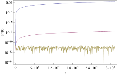
Figure 1: Comparison between the analytical and numerical solutions obtained using normal forms of 1st (upper curve), 3rd (central curve) and 5th (bottom curve) orders. The integration time is $T=10^{4}\pi$, the parameters are $\varepsilon=10^{-3}$, $\mu=10^{-3}$; the initial condition is set to $Y_{0}=\frac{1}{2}\left(\sqrt{5}+1\right)$, $X_{0}=0$.

5.3 Exponential stability estimates

In this section we present an application of the Theorem of Section 3 to the sample provided by the differential system (5). We first discuss the smallness conditions required for the parameters (Section 4.3.1) and then we compute the stability estimates (Section 4.3.2).

5.3.1 Bounds on the parameters

The bounds on the parameters $\varepsilon$ and $\mu$ are due to the smallness conditions imposed by the requirements to invert from original to intermediate variables, to invert from intermediate to new variables, to satisfy the non–resonance condition in the intermediate variables and the non–resonance condition in the new variables. With reference to the Appendix A, assuming $y_{0}=\frac{1}{2}\left(\sqrt{5}+1\right)$, $x_{0}=0$, $r_{0}=0.118$, $s_{0}=0.1$, $\delta_{0}=0.05$, $K=20$, one finds $\tilde{r}_{0}=0.113$, $\tilde{s_{0}}=0.05$, $\tilde{r}_{0}^{\prime}=0.056$, $R_{0}=0.057$, $S_{0}=0.025$, $a=0.09$ (the parameters are chosen so to optimize the result). Condition (28) requires that $\varepsilon\leq 1.2\cdot 10^{-4}$, while condition (33) imposes that $\varepsilon\leq 7.2\cdot 10^{-4}$ (no requirements are needed on $\mu$). Condition (4) is satisfied provided $\varepsilon\leq 1.2\cdot 10^{-4}$, $|\mu|\leq 2.0\cdot 10^{-4}$, while condition (37) requires that $\varepsilon\leq 3.0\cdot 10^{-3}$, $\eta\leq 4.75\cdot 10^{-3}$. In conclusion we obtain that all conditions are satisfied provided that $\varepsilon\leq 1.2\cdot 10^{-4}$ and $|\mu|\leq 2.0\cdot 10^{-4}$.

5.3.2 Stability estimates

The final step is to implement the estimates derived from the Theorem, keeping in mind that there are no Fourier modes of the form $h_{10}^{>K}$ in the sample (5). Let us write the transformation of the second component from original to final variables as $Y=y+T^{(N)}(y,x,t)$. For given $\varepsilon\leq\varepsilon_{0}$, $|\mu|\leq\mu_{0}$ and given $\lambda_{0}=\max(\varepsilon_{0},\mu_{0})$, we calculate the constant $C_{p}$ as $\left\|T^{(N)}\|_{r_{0},s_{0}}\right/\lambda_{0}$ and we define $r_{1}=C_{p}\lambda_{0}$. Taking $r_{2}$ of the same order of magnitude as $r_{1}$, we set $C_{t}={r_{2}}/C_{Y}$ with $C_{Y}=\left\|G_{N+1}\|_{R_{0},S_{0}}\right/\lambda_{0}^{N+1}$. For the variation in action space we set $\tilde{\rho}_{0}=2r_{1}+r_{2}\lambda_{0}$. We finally compute $\tau_{0}$ from (39). In conclusion we obtain that

$$\left\|y(t)-y(0)\right\|\leq\tilde{\rho}_{0}\quad{\rm for\ any}\quad t\leq T_{0}\equiv C_{t}e^{K\tau_{0}}\ .$$

$\begin{array}[]{lllll}\hline\cr\hline\cr N&2&3&4&5\\ \hline\cr\tau_{0}&0.851&1.277&1.703&2.129\\ \|G_{N+1}\|_{R_{0},S_{0}}&1.966\cdot 10^{-7}&5.147\cdot 10^{-10}&1.320\cdot 10^{-12}&2.053\cdot 10^{-15}\\ \|T_{N}\|_{r_{0},s_{0}}&3.815\cdot 10^{-4}&3.819\cdot 10^{-4}&3.819\cdot 10^{-4}&3.820\cdot 10^{-4}\\ C_{p}&1.908&1.909&1.909&1.910\\ C_{Y}&4.915&6.433\cdot 10^{1}&8.251\cdot 10^{2}&6.416\cdot 10^{3}\\ C_{t}&3.881\cdot 10^{-1}&2.968\cdot 10^{-2}&2.314\cdot 10^{-3}&2.977\cdot 10^{-4}\\ \tilde{\rho}_{0}&1.145\cdot 10^{-3}&1.146\cdot 10^{-3}&1.146\cdot 10^{-3}&1.146\cdot 10^{-3}\\ T_{0}&9.702\cdot 10^{6}&3.710\cdot 10^{9}&1.446\cdot 10^{12}&9.302\cdot 10^{14}\\ \hline\cr\hline\cr\end{array}$

Table 2: Stability results versus the normalization order $N$. For the definition of the constants see the text. The parameters are taken to optimize the stability time: $\varepsilon_{0}=1.2\cdot 10^{-4}$, $\mu_{0}=2.0\cdot 10^{-4}$, $y_{0}={1\over 2}(\sqrt{5}+1)$, $r_{0}=0.118$, $s_{0}=0.1$, $K=20$. Notice that in this table we fix $K$ and we let $\tau_{0}$ vary.

$\begin{array}[]{lllll}\hline\cr\hline\cr N&2&3&4&5\\ \hline\cr K&8&12&17&21\\ \|G_{N+1}\|_{R_{0},S_{0}}&1.970\cdot 10^{-7}&5.169\cdot 10^{-10}&1.329\cdot 10^{-12}&2.072\cdot 10^{{-15}}\\ \|T_{N}\|_{r_{0},s_{0}}&3.815\cdot 10^{-4}&3.819\cdot 10^{-4}&3.819\cdot 10^{-4}&3.820\cdot 10^{-4}\\ \lambda_{0}&2.0\cdot 10^{-4}&2.0\cdot 10^{-4}&2.0\cdot 10^{-4}&2.0\cdot 10^{-4}\\ C_{p}&1.908&1.909&1.909&1.910\\ C_{Y}&4.924&6.461\cdot 10^{1}&8.307\cdot 10^{2}&6.476\cdot 10^{3}\\ C_{t}&3.874\cdot 10^{-1}&2.955\cdot 10^{-2}&2.299\cdot 10^{-3}&2.949\cdot 10^{-4}\\ \tilde{\rho}_{0}&1.145\cdot 10^{-3}&1.146\cdot 10^{-3}&1.146\cdot 10^{-3}&1.146\cdot 10^{-3}\\ T_{0}&3.443\cdot 10^{6}&7.828\cdot 10^{8}&1.341\cdot 10^{12}&5.129\cdot 10^{14}\\ \hline\cr\hline\cr\end{array}$

Table 3: Stability results versus the normalization order $N$. For the definition of the constants see the text. The parameters are taken to optimize the stability time: $\varepsilon_{0}=1.2\cdot 10^{-4}$, $\mu_{0}=2.0\cdot 10^{-4}$, $y_{0}={1\over 2}(\sqrt{5}+1)$, $r_{0}=0.118$, $s_{0}=0.1$, $\tau_{0}=2$. Notice that in this table we fix $\tau_{0}$ and we let $K$ vary.

The actual values of the parameters, as a function of the normalization order $N$, are summarized in Table 2. The parameters $\varepsilon_{0}$ and $\mu_{0}$ are taken from the estimates on the smallness of the parameters (see Section 5.3.1), while $K$ was set equal to $20$.

Similar estimates can be obtained by fixing $\tau_{0}$ and calculating $K$ accordingly. Since $K$ also enters into the denominators of the non–resonance conditions (33) and (37), it will also influence the bounds on the smallness of the parameters. The results are shown in Table 3. Fixing $\tau_{0}=2$ the choice of $K$ depends on the order of normalization and on the bound on the smallness parameter $\lambda_{0}$, leading to a slightly different $K\tau_{0}$ compared to the values given in Table 2. The stability times in Tables 2 and 3 are of the same order of magnitude, since the values of $\mu$ and $\varepsilon$ are comparable at all orders. The stability estimates are checked for the parameters given in Table 3 at order 3 (whose stability time is compatible with the computer execution time) by comparison with a numerical simulation as shown in Figure 2. The integration time was set to be of the order of the stability time (i.e., we integrated up to $3.71\cdot 10^{9}$); we found that the deviation of the action is bounded as $5.629\cdot 10^{-4}$, while the analytical estimate provides $1.146\cdot 10^{-3}$ (the numerical deviation is therefore bounded with a safety factor $2$).

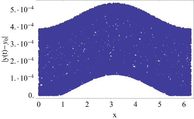
Figure 2: Numerical simulation of the original equations of motion for $3.71\cdot 10^{9}$ integration time. The parameters are taken from Table 2, 3rd column. The numerically found drift in action space is $5.629\cdot 10^{-4}$ and it is by a factor $2$ smaller than the upper bound obtained through the analytical estimate, which is equal to $1.146\cdot 10^{-3}$.

5.4 A system with oscillating energy

We conclude by providing an example of a differential system which admits oscillating energy. To be more precise, we consider the differential equations

$${}\dot{x} = y$$

$$\dot{y} = -\varepsilon\left(\sin(x-t)+\sin(x)\right)-\mu(y\sin(x)-\eta).$$

The Hamiltonian function for $\mu=0$ (in the extended phase space) reads as

$${}H(y,T,x,t)=\frac{y^{2}}{2}-\varepsilon\left(\cos(x-t)+\cos(x)\right)+T\ ,$$

where $T$ is the conjugated action to the time $t$. For $\mu\neq 0$ we get that the variation of the energy is given by

$${}\frac{d{H}}{dt}=\frac{\partial{H}}{\partial y}\dot{y}+\frac{\partial{H}}{\partial x}\dot{x}+\frac{\partial{H}}{\partial T}\dot{T}+\frac{\partial{H}}{\partial t}\dot{t}=\mu y^{2}\sin(x)-\mu y\eta\ .$$

Since the normal form equations will provide that $\eta=0$, we can conclude that the energy is oscillating. The normal form solution to second order provides the following expressions for the transformations:

$${}\psi_{10}(\tilde{y},\tilde{x},t) = \frac{\sin(\tilde{x}-t)}{\tilde{y}-1}+\frac{\sin(\tilde{x})}{\tilde{y}}$$

$$\psi_{20}(\tilde{y},\tilde{x},t) = -\frac{\sin(2\tilde{x}-t)}{2(\tilde{y}-1)\tilde{y}(2\tilde{y}-1)}-\frac{\sin(2\tilde{x}-2t)}{8(\tilde{y}-1)^{3}}-\frac{\sin(t)}{2(\tilde{y}-1)\tilde{y}}-\frac{\sin(2\tilde{x})}{8\tilde{y}^{3}}$$

$$\beta_{01}(Y,X,t) = \cos(X)$$

$$\alpha_{01}(Y,X,t) = \frac{\sin(X)}{Y}$$

$$\beta_{02}(Y,X,t) = -\frac{\cos(2X)}{2Y}$$

$$\beta_{11}(Y,X,t) = \frac{Y\cos(2X-t)}{2(Y-1)^{2}(2Y-1)}+\frac{(Y-2)\cos(t)}{2(Y-1)^{2}}-\frac{\cos(2X)}{4Y^{2}}$$

$$\alpha_{02}(Y,X,t) = -\frac{\sin(2X)}{4Y^{2}}$$

$$\alpha_{11}(Y,X,t) = -\frac{\sin(2X-t)}{2(Y-1)(2Y-1)^{2}}+\frac{(Y-3)\sin(t)}{2(Y-1)^{2}}-\frac{\sin(2X)}{8Y^{3}}\ .$$

The corresponding normal form at second order is given by:

$${}\dot{X} = Y+\frac{1-3Y+3Y^{2}-2Y^{3}}{2(Y-1)^{3}Y}\varepsilon^{2}+\frac{\varepsilon\mu}{2Y^{2}}+O_{2}(\varepsilon,\mu)$$

$$\dot{Y} = O_{2}(\varepsilon,\mu)\ .$$

We compare the solution of the normal form equations with the numerical solution by computing the error as in (42) for $\varepsilon_{0}=10^{-3}$, $\mu_{0}=10^{-3}$ and $Y_{0}=\frac{1}{2}\left(\sqrt{5}+1\right)$, $X_{0}=0$. Figure 3 (left panel) shows the error for the 1st (continuous line), 3rd (dashed line) and 5th (dotted line) order respectively, up to time $10^{4}\pi$; the oscillating behavior of the energy is given in the right panel of Figure 3. The numerical solution was again obtained using a 4th order Runge–Kutta integration scheme with fixed step size $\delta_{t}=10^{-2}$. We remark that the difference between the numerical and analytical solutions decreases as the order of the normal form increases. We conclude by mentioning that the bounds on the small parameters as well as the stability estimates can be determined as in Section 5.3.

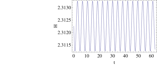
Figure 3: Left: relative error between the normal form and the numerical solution. We set $\varepsilon=10^{-3}$, $\mu=10^{-3}$ and $Y_{0}=\frac{1}{2}\left(\sqrt{5}+1\right)$; the evolution is in good agreement with the solution obtained from the normal form equations (continuous 1st, dashed 3rd, dotted 5th order normal form). Right: behavior of the energy of the system, which oscillates around a mean value with period $3.86$ .

6 Appendix A

We discuss the conditions which must be satisfied by the parameters $\varepsilon$, $\mu$, so that the transformation from original to intermediate variables can be inverted, as well as that from intermediate to final variables; moreover, we give conditions on the parameters so that the non–resonance conditions in the intermediate and final variables are satisfied. Such results rely on the following two lemmas which are proven in [29].

Lemma A.1. Let $y_{0}\in{\mathbb{R}}^{\ell}$, $(x,t)\in{\mathbb{T}}^{\ell+1}$, $r_{0}$, $s_{0}$, $\delta_{0}$ ($\delta_{0}<s_{0}$) be strictly positive parameters and let $g$ be a vector function holomorphic on the domain $D(y_{0},r_{0},s_{0})\equiv\{(y,x,t)\in{\mathbb{C}}^{2\ell+1}:\ \|y-y_{0}\|\leq r_{0}\ ,\ \max_{1\leq j\leq\ell}|\Im(x_{j})|\leq s_{0}\ ,\ |\Im(t)|\leq s_{0}\}$. Let us consider the equation

$$x^{\prime}=x+g(y,x,t)\ ;$$ (43)

if

$$C\|g\|_{r_{0},s_{0}}e^{2s_{0}}\delta_{0}^{-1}<1$$ (44)

for some positive constant $C$, then (43) can be inverted as

$$x=x^{\prime}+G(y,x^{\prime},t)\ ,$$

for a suitable function $G$ such that

$$\|G\|_{r_{0},s_{0}-\delta_{0}}\leq\|g\|_{r_{0},s_{0}}\ .$$

Lemma A.2. Let $y_{0}\in{\mathbb{R}}^{\ell}$, $(x,t)\in{\mathbb{T}}^{\ell+1}$ and let $r_{0}$, $s_{0}$, $\tilde{r}_{0}$ be strictly positive parameters with $r_{0}^{\prime}<r_{0}$; let $g$ be a vector function holomorphic on the domain $D(y_{0},r_{0},s_{0})\equiv\{(y,x,t)\in{\mathbb{C}}^{2\ell+1}:\ \|y-y_{0}\|\leq r_{0}\ ,\ \max_{1\leq j\leq\ell}|\Im(x_{j})|\leq s_{0}\ ,\ |\Im(t)|\leq s_{0}\}$. Let us consider the equation

$$y^{\prime}=y+g(y,x,t)\ ;$$ (45)

if

$$C\|g\|_{r_{0},s_{0}}{1\over{r_{0}-r_{0}^{\prime}}}<1$$ (46)

for some positive constant $C$, then (45) can be inverted as

$$y=y^{\prime}+G(y^{\prime},x,t)\ ,$$

for a suitable function $G$ such that

$$\|G\|_{r_{0}^{\prime},s_{0}}\leq\|g\|_{r_{0},s_{0}}\ .$$

We remark that a careful evaluation of the constant $C$ in (44) and (46) shows that it can be fixed as $C=70$.

6.1 Inversion of the conservative transformation

Let us recall the transformation (3) as

$$\tilde{x} = x+\psi_{y}^{(N)}(\tilde{y},x,t)$$

$$y = \tilde{y}+\psi_{x}^{(N)}(\tilde{y},x,t)\ ,$$ (47)

that we wish to invert as

$$x = \tilde{x}+\Gamma^{(x,N)}(\tilde{y},\tilde{x},t)$$

$$y = \tilde{y}+\Gamma^{(y,N)}(\tilde{y},\tilde{x},t)\ .$$ (48)

Let $\tilde{r}_{0}<r_{0}$, $\delta_{0}<s_{0}$, $\tilde{s}_{0}\equiv s_{0}-\delta_{0}$; the inversion of the first in (6.1) can be performed provided that

$$70\,\|\psi_{y}^{(N)}\|_{\tilde{r}_{0},s_{0}}e^{2s_{0}}\delta_{0}^{-1}<1\ ,$$

with

$$\|\Gamma^{(x,N)}\|_{\tilde{r}_{0},\tilde{s}_{0}}\leq\|\psi_{y}^{(N)}\|_{\tilde{r}_{0},s_{0}}\ .$$

The second in (6.1) is obtained from

$$y=\tilde{y}+\psi_{x}^{(N)}(\tilde{y},\tilde{x}+\Gamma^{(x,N)}(\tilde{y},\tilde{x},t),t)\equiv\tilde{y}+\Gamma^{(y,N)}(\tilde{y},\tilde{x},t)\ ,$$

where

$$\|\Gamma^{(y,N)}\|_{\tilde{r}_{0},\tilde{s}_{0}}\leq\|\psi_{x}^{(N)}\|_{\tilde{r}_{0},s_{0}}+\|\psi_{xx}^{(N)}\|_{\tilde{r}_{0},s_{0}}\|\Gamma^{(x,N)}\|_{\tilde{r}_{0},\tilde{s}_{0}}\ .$$

6.2 Non–resonance condition after the conservative normal form

Taking into account (3), we want that the non–resonance condition is satisfied in the intermediate variables, say for $a>0$:

$$|\omega(\tilde{y})\cdot k+m|>{a\over 2}\ ,\qquad|k|+|m|\leq K\ ,$$ (49)

where from (6.1) we get

$$\tilde{y}=y+\varepsilon R^{(N)}(y,x,t)\ ,$$ (50)

for a suitable function $R^{(N)}$. In fact, the second of (6.1) can be inverted as in (50) provided

$$70\,\|\psi_{x}^{(N)}\|_{\tilde{r}_{0},s_{0}}{1\over{\tilde{r}_{0}-\tilde{r}_{0}^{\prime}}}<1\ ,$$

for $\tilde{r}_{0}^{\prime}<\tilde{r}_{0}$ with

$$\varepsilon\|R^{(N)}\|_{\tilde{r}_{0}^{\prime},s_{0}}\leq\|\psi_{x}^{(N)}\|_{\tilde{r}_{0},s_{0}}\ .$$

Then we have

$$|\omega(\tilde{y})\cdot k+m|\geq|\omega(y)\cdot k+m|-\varepsilon K\|R^{(N)}\|_{\tilde{r}_{0}^{\prime},s_{0}}\|\omega_{y}\|_{r_{0}}\geq a-{a\over 2}={a\over 2}\ ,$$

provided

$$\varepsilon\leq{a\over{2K\|R^{(N)}\|_{\tilde{r}_{0}^{\prime},s_{0}}\|\omega_{y}\|_{r_{0}}}}\ .$$

6.3 Inversion of the dissipative transformation

Let us now discuss the inversion of (3) that we write for short as

$$X = \tilde{x}+\alpha^{(N)}(\tilde{y},\tilde{x},t)$$

$$Y = \tilde{y}+\beta^{(N)}(\tilde{y},\tilde{x},t)\ ;$$ (51)

we invert (6.3) as

$$\tilde{x} = X+\Delta^{(x,N)}(Y,X,t)$$

$$\tilde{y} = Y+\Delta^{(y,N)}(Y,X,t)\ ,$$

provided $\varepsilon$, $|\mu|$ are sufficiently small. In fact, the first of (6.3) can be inverted provided

$$70\,\|\alpha^{(N)}\|_{\tilde{r}_{0},\tilde{s}_{0}}\ e^{2\tilde{s}_{0}}\tilde{\delta}_{0}^{-1}<1\ ,$$

where $\tilde{\delta}_{0}<\tilde{s}_{0}$. Inverting the equation as

$$\tilde{x}=X+A^{(x,N)}(\tilde{y},X,t)\ ,$$

we have

$$\|A^{(x,N)}\|_{\tilde{r}_{0},\tilde{s}_{0}-\tilde{\delta}_{0}}\leq\|\alpha^{(N)}\|_{\tilde{r}_{0},\tilde{s}_{0}}\ .$$

Writing the second of (6.3) as

$$Y=\tilde{y}+\beta^{(N)}(\tilde{y},X+A^{(x,N)}(\tilde{y},X,t),t)\equiv\tilde{y}+B^{(y,N)}(\tilde{y},X,t)\ ,$$

we can invert it as

$$\tilde{y}=Y+\Delta^{(y,N)}(Y,X,t)\ ,$$

provided

$$70\,\|A^{(y,N)}\|_{\tilde{r}_{0},S_{0}}{1\over{\tilde{r}_{0}-R_{0}}}<1\ ,$$

with $S_{0}<\tilde{s}_{0}-\tilde{\delta}_{0}$, $R_{0}<\tilde{r}_{0}$, being

$$\|\Delta^{(y,N)}\|_{R_{0},S_{0}}\leq\|A^{(y,N)}\|_{\tilde{r}_{0},S_{0}}\ .$$

Notice that $A^{(y,N)}$ can be bounded as

$$\|A^{(y,N)}\|_{\tilde{r}_{0},S_{0}}\leq\|\beta^{(N)}\|_{\tilde{r}_{0},\tilde{s}_{0}}+\|\beta^{(N)}_{x}\|_{\tilde{r}_{0},\tilde{s}_{0}}\|A^{(x,N)}\|_{\tilde{r}_{0},S_{0}}\ .$$

6.4 Non–resonance condition after the dissipative normal form

We now turn to the fulfillment of the non–resonant condition in the new set of variables

$$|\omega(Y)\cdot k+m|>0\ ,\qquad|k|+|m|\leq K\ .$$

To this end, we use the transformation

$$Y=\tilde{y}+\beta^{(N)}(\tilde{y},\tilde{x},t;\varepsilon,\mu)$$

and using (49) one easily finds

$$|\omega(Y)\cdot k+m|\geq|\omega(\tilde{y})\cdot k+m|-K\|\omega_{y}\|_{r_{0}}\|\beta^{(N)}\|_{\tilde{r}_{0},\tilde{s}_{0}}>{a\over 2}-{a\over 4}\ ,$$

provided the following smallness condition on the parameters is satisfied:

$$K\,\|\omega_{y}\|_{r_{0}}\|\beta^{(N)}\|_{\tilde{r}_{0},\tilde{s}_{0}}<{a\over 4}\ .$$

7 Appendix B

Lemma B.1. Let $f=f(y,x,t)$ be an analytic function on the domain $C_{r_{0}}(A)\times C_{s_{0}}({\mathbb{T}}^{\ell+1})$. Let $f^{>K}(y,x,t)\equiv\sum_{(j,m)\in{\mathbb{Z}}^{\ell+1},|j|+|m|>K}\hat{f}_{jm}(y)\ e^{i(j\cdot x+mt)}$ and let $0<\sigma_{0}<s_{0}$. Then, there exists a constant $C_{a}\equiv C_{a}(\sigma_{0},K)$, such that

$$\|f^{>K}\|_{r_{0},s_{0}}\leq C_{a}\|f\|_{r_{0},s_{0}+\sigma_{0}}e^{-(K+1)\sigma_{0}}\ ,$$ (52)

with

$$C_{a}\equiv e^{(K+1){\sigma_{0}\over 2}}\left(\frac{1+e^{-{\sigma_{0}\over 2}}}{1-e^{-{\sigma_{0}\over 2}}}\right)^{\ell+1}\ .$$ (53)

Proof. From the properties of analytic functions, one has that

$$|\hat{f}_{jm}(y)|\leq\|f\|_{r_{0},s_{0}+\sigma_{0}}e^{-(s_{0}+\sigma_{0})(|j|+|m|)}\ .$$

Therefore one finds

$$\|f^{>K}\|_{r_{0},s_{0}} = \sum_{(j,m)\in{\mathbb{Z}}^{\ell+1},|j|+|m|>K}|\hat{f}_{jm}(y)|\ e^{s_{0}(|j|+|m|)}$$

$$\leq \|f\|_{r_{0},s_{0}+\sigma_{0}}\ \sum_{(j,m)\in{\mathbb{Z}}^{\ell+1},|j|+|m|>K}e^{-(s_{0}+\sigma_{0})(|j|+|m|)}e^{s_{0}(|j|+|m|)}$$

$$= \|f\|_{r_{0},s_{0}+\sigma_{0}}\ \sum_{(j,m)\in{\mathbb{Z}}^{\ell+1},|j|+|m|>K}e^{-\sigma_{0}(|j|+|m|)}\ .$$

Taking into account that

$$\sum_{(j,m)\in{\mathbb{Z}}^{\ell+1},|j|+|m|>K}e^{-\sigma_{0}(|j|+|m|)} \leq e^{-(K+1){\sigma_{0}\over 2}}\ \sum_{(j,m)\in{\mathbb{Z}}^{\ell+1},|j|+|m|>K}e^{-{\sigma_{0}\over 2}(|j|+|m|)}$$

$$\leq e^{-(K+1){\sigma_{0}\over 2}}\left(\sum_{p\in{\mathbb{Z}}}e^{-|p|{\sigma_{0}\over 2}}\right)^{\ell+1}$$

$$= e^{-(K+1){\sigma_{0}\over 2}}\left(\frac{1+e^{-{\sigma_{0}\over 2}}}{1-e^{-{\sigma_{0}\over 2}}}\right)^{\ell+1}\ ,$$

one obtains (52) with $C_{a}$ as in (53). $\Box$

Acknowledgments. We deeply thank Luca Biasco, Renato Calleja, Antonio Giorgilli and Jean–Christophe Yoccoz for very useful discussions and suggestions. We acknowledge the grants ASI “Studi di Esplorazione del Sistema Solare” and PRIN 2007B3RBEY “Dynamical Systems and Applications” of MIUR.

References

- [1] V.I. Arnold, Proof of a Theorem by A.N. Kolmogorov on the invariance of quasi-periodic motions under small perturbations of the Hamiltonian, Russ. Math. Surveys 18, 13–40 (1963)
- [2] V.I. Arnold (editor), Encyclopaedia of Mathematical Sciences, Dynamical Systems III, Springer–Verlag 3 (1988)
- [3] C. Beaugé, S. Ferraz–Mello, Resonance Trapping in the Primordial Solar Nebula: The Case of a Stokes Drag Dissipation, Icarus 103, 301–318 (1993)
- [4] G. Benettin, F. Fassó, M. Guzzo, Nekhoroshev–stability of L4 and L5 in the spatial restricted three–body problem, Reg. Chaotic Dyn. 3, 56–72 (1998)
- [5] G. Benettin, L. Galgani, A. Giorgilli, A Proof of Nekhoroshev’s Theorem for the stability times in nearly integrable Hamiltonian systems, Celest. Mech. Dyn. Astron. 37, 1–25 (1985)
- [6] G. Benettin, M. Guzzo, F. Fassó, Long term stability of proper rotations of the perturbed Euler rigid body, Commun. Math. Phys. 250, 133–160 (2004)
- [7] L. Biasco, L. Chierchia, Exponential stability for the resonant D’Alembert model of Celestial Mechanics, DCDS A 12, 569–594 (2005)
- [8] H.W. Broer, G.B. Huitema, M.B. Sevryuk, Quasi–periodic motions in families of Dynamical systems, Lecture Notes in Mathematics, Springer–Verlag (1996)
- [9] H.W. Broer, C. Simó, J.C. Tatjer, Towards global models near homoclinic tangencies of dissipative diffeomorphisms, Nonlinearity 11, no. 3, 667–770 (1998)
- [10] R. Calleja, A. Celletti, Breakdown of invariant attractors for the dissipative standard map, CHAOS 20, issue 1, 013121 (2010)
- [11] R. Calleja, A. Celletti, R. de la Llave, KAM theory for conformally symplectic systems, Preprint 2011, available on the Mathematical Physics Preprint Archive: mp_arc 11–188
- [12] A. Celletti, Stability and Chaos in Celestial Mechanics, Springer-Praxis 2010, XVI, 264 pp., Hardcover ISBN: 978-3-540-85145-5
- [13] A. Celletti, L. Chierchia, Quasi–periodic attractors in Celestial Mechanics, Arch. Rat. Mech. Anal. 191, no. 2, 311–345 (2009)
- [14] A. Celletti, S. Di Ruzza, Periodic and quasi–periodic attractors of the dissipative standard map, DCDS–B 16, n. 1, 151–171 (2011)
- [15] A. Celletti, L. Ferrara, An application of the Nekhoroshev theorem to the restricted three–body problem, Cel. Mech. Dyn. Astr. 64, 261–272 (1996)
- [16] A. Celletti, A. Giorgilli, On the stability of the Lagrangian points in the spatial restricted problem of three bodies, Cel. Mech. Dyn. Astr. 50, 31–58 (1991)
- [17] A. Celletti, C. Lhotka, Stability of nearly–Hamiltonian systems with resonant frequency, Preprint 2011
- [18] A. Celletti, C. Lhotka, A comparison of numerical integration methods in nearly–Hamiltonian systems, work in progress 2012
- [19] A. Celletti, R.S. MacKay, Regions of non–existence of invariant tori for spin–orbit models, Chaos 17, 043119, pp. 12 (2007)
- [20] A. Celletti, L. Stefanelli, E. Lega, C. Froeschlé, Global dynamics of the regularized restricted three–body problem with dissipation, Cel. Mech. Dyn. Astr. 109, 265–284 (2011)
- [21] A. Delshams, A. Guillamon, J.T. Lazaro, A pseudo-normal form for planar vector fields, Qual. Theory Dyn. Syst. 3, n. 1, 51–82 (2002)
- [22] J. Henrard, A Survey of Poisson Series Processors , Cel.Mech. 45, 245–253 (1989)
- [23] C. Efthymiopoulos, Z. Sándor, Optimized Nekhoroshev stability estimates for the Trojan asteroids with a symplectic mapping model of co-orbital motion, MNRAS 364, n. 1, 253–271 (2005)
- [24] F. Fassò, Lie series method for vector fields and Hamiltonian perturbation theory, J. Appl. Math. Phys. 41 843?864 (1990)
- [25] U. Feudel, C. Grebogi, B.R. Hunt, J.A. Yorke, Map with more than 100 coexisting low–period periodic attractors, Phys. Rev. E 54, 71-?81 (1996)
- [26] A. Giorgilli, Effective stability in Hamiltonian systems in the light of Nekhoroshev’s theorem, Integrable Systems and Applications, Springer–Verlag, Berlin, New York, 142-153 (1989)
- [27] A. Giorgilli, A. Delshams, E. Fontich, L. Galgani, C. Simó, Effective stability for a Hamiltonian system near an elliptic equilibrium point, with an application to the restricted three body problem, J. Diff. Eq. 77, 167–198 (1989)
- [28] A. Giorgilli, Ch. Skokos, On the stability of the Trojan asteroids, Astron. Astroph. 317, 254–261 (1997)
- [29] G. Gallavotti, The Elements of Mechanics, Springer–Verlag (1983)
- [30] G. Ioos, E. Lombardi, Polynomial normal forms with exponentially small remainder for analytic vector fields, J. Diff. Eq. 212, 1–61 (2005)
- [31] G. Ioos, E. Lombardi, Approximate invariant manifolds up to exponentially small terms, J. Diff. Eq. 248, 1410–1431 (2010)
- [32] A.N. Kolmogorov, On the conservation of conditionally periodic motions under small perturbation of the Hamiltonian, Dokl. Akad. Nauk. SSR 98, 527–530 (1954)
- [33] C. Lhotka, C. Efthymiopoulos, R. Dvorak, Nekhoroshev stability at or in the elliptic–restricted three–body problem - application to Trojan asteroids, MNRAS 384, no. 3, 1165–1177 (2008)
- [34] A.P. Markeev, The stability of the plane motions of a rigid body in the Kovalevskaya case, J. Appl. Math. Mech. 65, n.1, 47–54 (2001)
- [35] J. Moser, On invariant curves of area–preserving mappings of an annulus, Nach. Akad. Wiss. Göttingen, Math. Phys. Kl. II 1, 1–20 (1962)
- [36] N.N. Nekhoroshev, An exponential estimate of the stability time of near–integrable Hamiltonian systems, Russ. Math. Surveys 32, no. 6, 1–65 (1977)
- [37] N.N. Nekhoroshev, Exponential estimates of the stability time of near-integrable Hamiltonian systems 2, Trudy Sem.Petrovos. 5, 5–65 (1979)
- [38] J. Pöschel, Nekhoroshev’s estimates for quasi–convex Hamiltonian systems, Math. Z. 213, 187–216 (1993)
- [39] D. Ruelle, Chaotic evolution and strange attractors, Cambridge University Press (1989)