Onset of Localization in Heterogeneous Interfacial Failure

Abstract

We study numerically the failure of an interface joining two elastic materials under load using a fiber bundle model connected to an elastic half space. We find that the breakdown process follows the equal load sharing fiber bundle model without any detectable spatial correlations between the positions of the failing fibers until localization sets in. The onset of localization is an instability, not a phase transition. Depending on the elastic constant describing the elastic half space, localization sets in before or after the critical load causing the interface to fail completely, is reached. There is a crossover between failure due to localization or failure without spatial correlations when tuning the elastic constant, not a phase transition. Contrary to earlier claims based on models different from ours, we find that a finite fraction of fibers must fail before the critical load is attained, even in the extreme localization regime, i.e. for very small elastic constant. We furthermore find that the critical load remains finite for all values of the elastic constant in the limit of an infinitely large system.

The joining of interfaces, e.g. by welding or gluing, is an important part of everyday technology, a technology that has been refined through the centuries. When joined interfaces are subject to excessive loads, failure occurs. Often it is not the joints themselves that fail, but the material that surrounds them, as the joints themselves are the stronger.

The aim of this work is, however, not to study failure of such joints with improvement of technology in mind. Rather, we take the point of view that failure of a heterogeneous joined interface provides a simplified model for fracture in bulk materials. Such an idea is not new. Schmittbuhl et al. srvm95 and Schmittbuhl and Måløy sm97 studied, first computationally, then experimentally, the roughness of the fracture front moving through a sintered interface between two Plexiglas plates that are being plied apart in a mode-I fashion. The study of the fluctuations of this fracture front provides much insight into the much more complex morphology of three-dimensional fracture surfaces bb11 .

We focus on the phenomenon of localization in this work. Local failure occurs either because the material is weaker at that spot or because it is more loaded there than elsewhere. Differences in local strength is due to heterogeneities. Differences in loading is due to structure in the stress field. If we assume that the interface is loaded uniformly — the local stress field will be quite uniform. Local failure will occur because of material weakness. For the simple reason that the further away we search from a point where a failure has occurred, the weaker the weakest spot we have found so far will be, localization is disfavored. Heterogeneity in strength induces a “repulsion” between the local failures. However, when failed areas build up, local stress is concentrated at the rim of the failed areas making these regions liable to fail. Heterogeneity in the stress field induces an “attraction” between local failures.

Localization occurs when attraction wins over repulsion. A transition in the failure process occurs at this point. What is the nature of this transition? As we shall demonstrate, it is not a phase transition, but a crossover phenomenon.

When localization sets in immediately in the breakdown process, it is normally expected that the system is infinitely fragile in the limit of infinitely large system: As soon as a single fiber breaks at a given load, the entire system breaks down at that load phc10 . As we will demonstrate, this is not the case here.

We base our work on the discretized model for interfacial failure proposed by Batrouni et al. bhs02 . A square array of $L\times L=N$ linearly elastic fibers placed a distance $a$ apart connects a stiff half-space with a linearly elastic half space characterized by a Young modulus $E$ and a Poisson ratio $\nu$ (which we assume a typical value of $0.25$ in the following). Each fiber, indexed by $i$, has an elastic constant $k$ and fails irreversibly if it is elongated beyond an individual threshold value $t_{i}$. The threshold values are drawn from a uniform distribution on the unit interval.

The separation of the two half spaces are controlled by displacing the hard medium by a distance $D$ orthogonal to the interface where the fibers sit. Fiber $i$ then experiences a force

$$f_{i}=-k(u_{i}-D)\;,$$ (1)

where $u_{i}$ is the local displacement of the softer half space at the position of fiber $i$. The forces from the fibers are transmitted through the softer elastic medium via the Green function l29 ; j85 ; ll86

$$u_{i}=\sum_{j}G_{ij}f_{i}\;,$$ (2)

where

$$G_{ij}=\frac{1-\nu^{2}}{\pi Ea^{2}}\iint^{a/2}_{-a/2}\frac{dx^{\prime}dy^{\prime}}{|\vec{r}_{i}(x,y)-\vec{r}_{j}(x^{\prime},y^{\prime})|}\;.$$ (3)

$\vec{r}_{i}-\vec{r}_{j}$ denotes the distance between fibers $i$ and $j$ at positions $\vec{r}_{i}$ and $\vec{r}_{j}$ respectively.

The Green function (3) is modified by the presence of boundaries due to the finite size $(La)\times(La)=Na^{2}$ of the interface. We assume periodic boundary conditions and take into account the first reflected images.

We note that if distances are measured in units of $a$, the Green function (3) is proportional to $(Ea)^{-1}$. Likewise, from Eq. (1), we see that the elastic constant of the fibers, $k$ must be proportional to $a^{2}$. Hence, if we change the linear size of the system, $(La)\to\lambda(La)$, while keeping the discretization $a$ fixed, we change only $L\to\lambda L$ in the model whereas we keep the parameters $Ea$ and $k$ fixed. On the other hand, if we change the discretization $a\to a/\lambda$ while leaving the size of the system fixed, we change $L\to\lambda L$ and the parameters $(Ea)\to(Ea)\lambda$ and $k\to k/\lambda^{2}$.

A given fiber breaks irreversibly (its elastic constant is set to zero) if stretched beyond a threshold value assigned from a spatially uncorrelated probability distribution. We choose the simplest: a uniform distribution. The model is quasi-static, and in lieu of time, we measure the fraction of fibers that have broken, denoted by $p$. The load carried by the system is $\sigma(p)=\sum_{i}f_{i}/N$, and when $\sigma$ reaches its maximum, any extra load will result in a complete catastrophic failure. We denote this the critical load, $\sigma_{c}$, and the corresponding $p_{c}$, the failure point.

In the limit of $(Ea/L)\to\infty$, the model becomes identical to the equal load sharing fiber bundle model (ELS) phc10 ; p26 ; d45 . On the other hand, for small values of $(Ea/L)$, it does not approach any existing models. Models do exist, e.g. the local load sharing fiber bundle model (LLS) hp81 , where the nearest surviving fibers absorbs the entire load that a fiber was carrying when failing. Another model, introduced by Hidalgo et al. hmkh02 , distributes the added load around a failed fiber as a power law in the distance from the failed fiber. In both models, there is no elastic response by the planes defining the interface.

We have studied systems of size $L=256$, $L=128$, $L=64$, $L=32$ $L=16$ and $L=8$ with $10$, $100$, $1000$, $10000$, $10000$ and $10000$ samples respectively. We explore a range of elastic constants $e\equiv(Ea/L)$ in the range $e_{\text{soft}}\leq e\leq e_{\text{stiff}}$ where $e_{\text{soft}}=2^{-17}=7.63\times 10^{-6}$ and $e_{\text{stiff}}=2^{6}=32$.

In order to visualize localization, we record the square distance between consecutively failing fibers, $\Delta r^{2}$. If the positions of the failing are completely random, as is the case in the ELS fiber bundle model, the average distance is $\langle\Delta r^{2}\rangle^{1/2}=L/\sqrt{6}\approx 0.408L$. We show in Fig. 1 a succession of histograms of $(\Delta r^{2})^{1/2}$. That is, we

record $\Delta r^{2}(n)$ as a function of the number of failed fibers, $n=pN$ — our “time” parameter. We then sum the number of times $\Delta r(n)$ has had a particular value $(\Delta r^{2})^{1/2}$ at $n$ for several independent simulations, hence creating a histogram for each $n$. Darker colors signifies more hits at that value of $(\Delta r)^{1/2}$. The curve shows the average value $\langle\Delta r^{2}(n)\rangle^{1/2}$. With $L=128$, we see that for the four different elastic constants $e$ that we show, $e=32$, $e=2^{-3.678}$ (this value is chosen to make the figure comparable to the results in Batrouni et al. bhs02 , where $L=128$, $E=10$, and $a=1$, which gives $e=0.0781=2^{-3.678}$.) $e=2^{-6}$ and $e=2^{-17}$, $\langle\Delta r^{2}(n)\rangle^{1/2}$ starts out being close to the ELF fiber bundle model value 52.26. The vertical line in each figure shows the failure point $n_{c}=p_{c}N$.

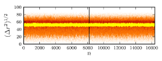
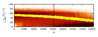
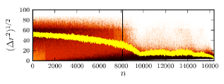
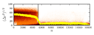
Figure 1: (Color online.) Histogram over the distance between consecutively failing fibers, $(\Delta r^{2}(n))^{1/2}$, as function of the number of failed fibers $n=pN$. Darker colors correspond to higher density. The vertical bar indicates the failure point, $p_{c}N$. The curve shows the running average $\langle\Delta r^{2}(n)\rangle^{1/2}$. In all figures, $L=128$. 100 simulations was used to construct the histogram. From top to bottom, $e=32$, $e=2^{-3.678}=0.0781$, $e=2^{-6}=0.0156$ and $e=2^{-17}=7.63\cdot 10^{-6}$.

Rising the value if the elastic constant $e$ above $e_{\text{stiff}}$ or below $e_{\text{soft}}$, will not lead to changes from the uppermost and lowermost panels in Fig. 1. At the highest value of $e$, the system behaves as the ELS fiber bundle model throughout the entire breakdown process: The average distance between consecutively failing fibers, $\langle\Delta r^{2}(n)\rangle^{1/2}$ remains constant throughout the process. The ELS fiber bundle model predicts $p_{c}=1/2$ so that $n_{c}=8192$.

As the system gets softer, both $\langle\Delta r^{2}(n)\rangle^{1/2}$ and $n_{c}$ decrease. We see in three lower panels in Fig. 1 that there is an abrupt change in $\langle\Delta r^{2}(n)\rangle^{1/2}$ for some range of $n$ values. This is localization. We also see that the failure point does not fall to zero as $e$ is lowered. Even for the smallest value in Fig. 1, $e=e_{\text{soft}}=2^{-17}$, $n_{c}$ is significantly different from zero.

Fig. 2 shows the failure point $p_{c}$ as a function of the inverse of the logarithm of total number of fibers, $1/\log_{10}(N)$. From this figure, we may extrapolate the value of $p_{c}$ in the limit of infinitely large system. We find $p_{c}(N\to\infty)=p_{c}^{\infty}=0.16$ when $e=e_{\text{soft}}$ and $p_{c}^{\infty}=0.5$ when $e=e_{\text{stiff}}$. Likewise, we may extrapolate the critical load $\sigma_{c}$ — see the insert in the figure. We find through extrapolation that $\sigma_{c}^{\infty}=0.17$ for $e=e_{\text{soft}}$ and $\sigma_{c}^{\infty}=0.25$ for $e=e_{\text{stiff}}$, the value expected for the ELS fiber bundle model.

It is a surprising result that neither $p_{c}^{\infty}$ nor $\sigma_{c}^{\infty}$ are zero for small value of $e$. The LLS fiber bundle model predicts that $\sigma_{c}\sim 1/\log_{10}(N)$ with $\sigma_{c}^{\infty}=0$ zd95 ; khh97 . Hidalgo et al. hmkh02 present numerical evidence that their model also has $\sigma_{c}^{\infty}=0$. Hence, in both of these models, $p_{c}^{\infty}=0$.

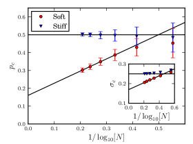
Figure 2: (Color online.) Finite size analysis of failure point and critical loading. Both $p_{c}$ (main plot) and $\sigma_{c}$ (encapsulated) is plotted against $1/\log_{10}[N]$, for $N=8^{2}=256$ to $N=256^{2}=65536$ and both have finite values for any $N$. The slope of the soft systems are $\alpha_{p_{c}}=0.68$ and $\alpha_{\sigma_{c}}=0.16$.

Batrouni et al. bhs02 studied the structure of the clusters of failed fibers at $p_{c}$, claiming that at the failure point, they are distributed according to a power law with exponent -1.6. This would indicate a critical point at $p=p_{c}$.

Referring to Fig. 1, we see that for $e=e_{\text{stiff}}=32$, the system behaves as the ELS fiber bundle model where the position of the fibers that fail bear no correlations among themselves. It is clear when observing the average distance between consecutively failing fibers, $\langle\Delta r(n)^{2}\rangle^{1/2}$ which essentially remains close to the ELS fiber bundle, where $\langle\Delta r^{2}(n)\rangle^{1/2}=L/\sqrt{6}$. Hence, we expect that the clusters follow percolation theory sa94 . In Fig. 3 we show the density of of the largest cluster of failed fibers, $s^{*}$, as a function of $p$ for $e=e_{\text{stiff}}$ and $e=e_{\text{soft}}$. In the case of the soft system, we see that at $p\approx 0.25$, the largest cluster becomes visible and grows essentially linearly with $p$. This behavior is due to localization. When $p$ approaches 1, there are jumps in $s^{*}$, because of coalescence of clusters. On the other hand, when $e=e_{\text{stiff}}$, we see behavior consistent with percolation theory. When $p$ is in the vicinity of $p=0.59274$, the site percolation threshold on the square lattice fdb08 , $s^{*}$ shoots up and thereafter evolve linearly in $p$.

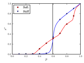
Figure 3: (Color online.) Density of the largest cluster of failed fibers, $s^{*}$, as a function of the damage $p$ for $e=e_{\text{stiff}}$ and $e=e_{\text{soft}}$. Here $L=128$. The vertical bar indicates the percolation point $p=0.59274$.

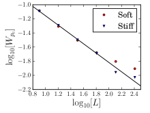
Figure 4: (Color online.) Fluctuations of $p_{c}$, $W_{c}=\sqrt{\langle p_{c}^{2}\rangle-\langle p_{c}\rangle^{2}}$ plotted against $L$ for $L=8$ to $L=256$. The slope of the black line is $-2/3$. The stiff system follows the slope, while the soft systems deviates.

The failure point at which the system fails catastrophically, $p_{c}$, occurs long before the jump in $s^{*}$ for $e=e_{\text{stiff}}$. This is an indication that the system is not critical at the failure point. Schmittbuhl et al. shb03 measured the fluctuations of the failure point as a function of the system size, finding $\Delta p_{c}\sim 1/L^{0.65}$. This is consistent with the GLS fiber bundle model. Daniels and Skyrme ds89 showed that the statistical distribution of the critical elongation in the GLS fiber bundle model has has the form

$$\rho(u_{c})du_{c}=N^{1/3}f[CN^{1/3}(u_{c}-\langle u_{c}\rangle)]du_{c}\;,$$ (4)

$C$ is a constant only dependent on the threshold distribution and $u_{c}$ is the critical elongation. This leads immediately to

$$\Delta p_{c}\sim\langle(u_{c}-\langle u_{c}\rangle)^{2}\rangle^{1/2}\sim N^{-1/3}=L^{-2/3}\;,$$ (5)

where we have used the assumption that the threshold distribution is uniform in the vicinity of $\langle u_{c}\rangle$ in relating $p_{c}$ to $u_{c}$. From Fig. 4 we can see that the stiff system scales as $L^{-2/3}$, while the soft systems deviates. We conclude that we cannot detect spatial correlation in the failure process beyond an uncorrelated percolation process for $e=e_{\text{stiff}}$.

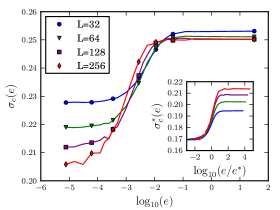
Figure 5: (Color online.) The critical load, $\sigma_{c}$, plotted against $\log_{10}(e)$ for several system sizes. The insert shows the rescaled $\sigma_{c}^{*}$ is plotted against $\log_{10}(e/e^{*})$, demonstrating data collapse.

We now proceed to study the onset of localization. Fig. 5 shows the critical load $\sigma_{c}$ as a function of $e$ for systems of size $L=32$ to $L=256$. As $e$ decreases, we observe that $\sigma_{c}$ drops from the ELS fiber bundle value, goes through a crossover and ends in a stable $\sigma_{c}$ for each $L$ in the soft regime. We define $e^{*}$ by setting

$$\sigma_{c}(e^{*})=\frac{1}{2}\left(\sigma_{c}(e_{\text{stiff}})+\sigma_{c}(e_{\text{soft}})\right)\;.$$ (6)

We then define

$$\sigma_{c}^{*}(e)=\sigma_{c}(e)-\frac{\alpha_{\sigma_{c}}}{\log_{10}[N]}\;.$$ (7)

We show $\sigma_{c}^{*}(e)$ vs. $\log_{10}(e/e^{*})$ in the insert in Fig. 5. As the correction term $-\alpha_{\sigma_{c}}/\log_{10}[N]\rightarrow 0$ in the macroscopic limit, we know that the curve never grow past $\sigma_{c}(e^{*})=0.25$. The largest gradient in $\sigma_{c}{e}$ seem to converge around

$$\frac{\Delta\sigma_{c}(e)}{\Delta\log_{10}[e/e^{*}]}=0.03,$$ (8)

and the shape of the curve is kept. The onset of localization is not a phase transition, but a crossover: there are no divergences anywhere in the derivative of this curve.

The following picture then emerges: For a given elastic constant, $e$, the breakdown process starts out as described by the ELS fiber bundle model. The spatial correlations between the failing fibers seems to be so weak that it can be described as an uncorrelated percolation process. If the elastic constant $e$ is large enough, the system will undergo both the ELS fiber bundle model failure point and the percolation transition. Depending on the threshold distribution, the ordering of the two events, the ELS failure point and the percolation transition, may be reversed. With lower elastic constant, localization sets in and breaks off the ELS fiber bundle breakdown process. When localization sets in, all failure activity is then essentially limited to the rim of a growing cluster of failed fibers. The onset of localization is an instability, not a phase transition.

We thank M. Grøva, S. Pradhan, S. Sinha and B. Skjetne for useful discussions. This work was partially supported by the Norwegian Research Council through grant no. 177591. We thank NOTUR for allocation of computer time.

References

- (1) J. Schmittbuhl, S. Roux, J. P. Vilotte and K. J. Måløy, Phys. Rev. Lett. 74, 1787 (1995).
- (2) J. Schmittbuhl and K. J. Måløy, Phys. Rev. Lett. 78, 3888 (1997).
- (3) D. Bonamy and E. Bouchaud, Phys. Rep. 498, 1 (2011).
- (4) S. Pradhan, A. Hansen and B. K. Chakrabarti, Rev. Mod. Phys. 82, 499 (2010).
- (5) G. G. Batrouni, A. Hansen and J. Schmittbuhl, Phys. Rev. E, 65, 036126 (2002).
- (6) A. E. H. Love, Phil. Trans. R. Soc. A 228 377 (1929).
- (7) K. L. Johnson, Contact Mechanics (Cambridge University Press, Cambridge, 1985).
- (8) L. D. Landau, L. P. Pitaevskii, E. M. Lifshitz and A. M. Kosevich, Theory of Elasticity, 3rd Edition (Clarendon Press, Oxford, 1986).
- (9) F. T. Peirce, J. Text. Ind. 17, 355 (1926).
- (10) H. E. Daniels, Proc. Roy. Soc. London, Ser. A 183, 405 (1945).
- (11) D. G. Harlow and S. L. Phoenix, Int. J. Fract. 17, 601 (1981).
- (12) R. C. Hidalgo, Y. Moreno, F. Kun and H. J. Herrmann, Phys. Rev. E, 65, 046148 (2002).
- (13) S. D. Zhang and E. J. Ding, J. Phys. A 28, 4323 (1995).
- (14) M. Kloster, A. Hansen and P. C. Hemmer, Phys. Rev. E 56, 2615 (1997).
- (15) D. Stauffer and A. Aharony, Introduction to Percolation Theory (Taylor and Francis, London, 1994).
- (16) X. Feng, Y. Deng and H. W. J. Blöte, Phys. Rev. E, 78, 031136 (2008)
- (17) J. Schmittbuhl, A. Hansen and G. G. Batrouni, Phys. Rev. Lett. 90, 045505 (2003).
- (18) H. E. Daniels and T. H. R. Skyrme, Adv. Appl. Prob. 21, 315 (1989).