Quantum Cournot equilibrium for the Hotelling-Smithies model of product choice

Abstract

This paper demonstrates the quantization of a spatial Cournot duopoly model with product choice, a two stage game focusing on non-cooperation in locations and quantities. With quantization, the players can access a continuous set of strategies, using continuous variable quantum mechanical approach. The presence of quantum entanglement in the initial state identifies a quantity equilibrium for every location pair choice with any transport cost. Also higher profit is obtained by the firms at Nash equilibrium. Adoption of quantum strategies rewards us by the existence of a larger quantum strategic space at equilibrium.

I Introduction

Quantum entanglement, a physical resource, plays a vital role in quantum information theory: when used as a resource it performs various tasks which seem rather impossible for classical resources. In this regard quantum game theory is no exception, where the concept of quantum entanglement has been used for the benefit of quantum game over a classical one. Quantum game theory was first introduced by Meyer Mey99 , who showed that a player can always beat his classical opponent by adopting quantum strategies. Since then there has been a great deal of theoretical efforts to extend the classical game theory into the quantum domain which established the fact that quantum games are more efficient than it’s classical counterpart at least in terms of information transfer EWL99 ; BH01 ; LDM02 ; HFM10 . Recently, successful accomplishment of the experimental realization of quantum games PSWZ07 ; SFWKWH10 ; DLXSWZH02 on NMR quantum computer has increased the attention on this topic.

In the literature of quantum games, one may note that the mostly studied quantum games focus on games in which the players have finite number of strategies. But in the economics of real life, there are games in which the players can access to a continuous set of strategies ball , a classic example of which is the Cournot’s duoploy, a game which describes market competition. The intimate connection between the game theory and the theory of quantum communication motivated Li et al LDM02 to analyse the quantization of Cournat’s dupoly using continuous variable quantum system. Extending this idea we have studied the quantum equilibrium for the Hotelling-Smithies model of product choice, which is a spatial Cournot duopoly with transport cost and price indiscrimination hotelling ; Smi41 . Quantization of the game shows that in equilibrium, the gain in the quantum domain is more, when the transportation cost is low. For higher transport costs, the difference between the quantum and classical profit is negligible. We have also shown that if the consumers are supplied with a $traveling$ $allowance$ to reach the seller, the optimal quantum strategic space becomes larger than the classical optimum strategic space.

In Section II we recapitulate the classical model of Hotelling-Smithies with product choice. Section III is devoted to the study the quantum version of the classical game and also deals with the benefit of the quantum game over the classical one. In Section IV we treat the game with travelling allowance instead of transport cost. We end with a conclusion.

II Classical Model of Hotelling-Smithies with product choice

Hotelling hotelling was the first to suggest that the competition between oligopolistic sellers result in consumers being offered products with an excessive sameness, where individual demand is perfectly inelastic. His analysis was extended by Smithies Smi41 to a case in which demand is inelastic and firms compete in quantities. It has been recognised that Cournot competition, which is quantity setting game, gives rise to different equilibria than the Betrand model of competition which is price setting game. We investigate the Hotelling-Smithies model of product choice and study the Cournot equilibria for spatial duopolists which are not able to price discriminate between their consumers. The inability to price discriminate may arise for two different situations: if consumers travel to the seller to collect the goods, or if the seller is unable to customize the product to the individual consumer’s desires.

Let us first describe our model where two firms indexed 1 and 2, are assumed to choose locations on a linear market normalized to unit length. Their locations, as measured by their distances from the left side market boundary, are denoted by $r_{1}$ and $r_{2}$ respectively. From the symmetry we can assume $0\leq r_{1}\leq r_{2}\leq 1$. According to the strategy of this two-stage game, these two firms can sell a product that is homogeneous in all characteristics other than the location at which it is available. Production cost is normalized to zero for both of them and the firms are able and willing to supply the entire market. They also simultaneously decide that the firm i(i=1,2) will produce the product of quantity $q_{i}$ and sell them with price $p_{i}$ (per unit of product). We also consider that the consumers are distributed uniformly with unit density over the entire linear market. Consumer inverse demand function is linear and is given by q(s)=1-p(s), where p is the price, q is the supply and s denote the location of the consumer. Inverse demand function and the positivity of q(s) and p(s) demand that $q(s),p(s)\leq 1$. If t(assumed linear in distance and quantity transported) is the transportation cost per unit length then the consumer need to pay the price $p_{i}+t|s-r_{i}|$ for per unit product, if he want to purchase the good from the i-th firm. It is very natural that every consumer intends to purchase the good with lower price.

To solve the competitive game in the market we confine our attention to a two stage game Smi41 ; chap7 . The firms first choose locations and then quantities where the second stage identifies the optimal quantity for any pair of locations of the firms. In the first stage the equilibrium locations are derived in the belief that the second stage choices will be an equilibrium quantity pair for the second stage subgame. A pure strategy subgame perfect Nash equlibrium for the two-stage quantity location Cournot game is defined as a pair of locations $(r_{1}^{c},r_{2}^{c})$ and a quantity pair $(q_{1}^{c}(r_{1}^{c},r_{2}^{c}),q_{2}^{c}(r_{1}^{c},r_{2}^{c}))$ such that

$$\Pi_{1}((q_{1}^{c}(r_{1}^{c},r_{2}^{c}),q_{2}^{c}(r_{1}^{c},r_{2}^{c})),r_{1}^{c},r_{2}^{c})\geq\Pi_{1}((q_{1}^{c}(r_{1},r_{2}^{c}),q_{2}^{c}(r_{1},r_{2}^{c})),r_{1},r_{2}^{c})~{}~{}~{}\forall~{}r_{1}\in[0,1]$$ (1)

and

$$\Pi_{2}((q_{1}^{c}(r_{1}^{c},r_{2}^{c}),q_{2}^{c}(r_{1}^{c},r_{2}^{c})),r_{1}^{c},r_{2}^{c})\geq\Pi_{2}((q_{1}^{c}(r_{1}^{c},r_{2}),q_{2}^{c}(r_{1},r_{2})),r_{1},r_{2})~{}~{}~{}\forall~{}r_{2}\in[0,1]$$ (2)

where

$$\Pi_{1}((q_{1}^{c}(r_{1},r_{2}),q_{2}^{c}(r_{1}^{c},r_{2}^{c})),r_{1}^{c},r_{2}^{c})\geq\Pi_{1}(q_{1},q_{2}^{c}(r_{1},r_{2}),r_{1},r_{2})~{}~{}\forall~{}q_{1}\geq 0~{}\rm{and}~{}r_{1},r_{2}\in[0,1]$$ (3)

and

$$\Pi_{2}((q_{1}^{c}(r_{1},r_{2}),q_{2}^{c}(r_{1},r_{2})),r_{1},r_{2})\geq\Pi_{2}(q_{1}^{c}(r_{1},r_{2}),q_{2}^{c}(r_{1},r_{2})),r_{1},r_{2}~{}~{}\forall~{}q_{2}\geq 0~{}\rm{and}~{}r_{2}\in[0,1]$$ (4)

The quantity subgame (1) and (2) can be solved for two different cases: perfect agglomeration where $r_{1}=r_{2}$, which is a symmetric case and a general case where there is no perfect agglomeration. In our model, we consider the case of non agglomeration and also choose $r_{1}<r_{2}$ with $r_{1}\leq 0.5$ and $r_{2}\geq 0.5$. The firms are not agglomerated, the products are perceived by consumers as being differentiated by location. We do not consider the market overlap, given the outputs $q_{i}$ of the two firms, the market clearing condition will determine the mill prices $p_{i}$ (i=1,2). If $r$ is the market boundary between two firms then,

$$p_{1}+t|r-r_{1}| = p_{2}+t|r-r_{2}|$$

$$\mbox{or, ~{}~{}~{}~{}~{} }r = \frac{p_{2}-p_{1}}{2t}+\frac{r_{1}+r_{2}}{2}$$ (5)

The quantity $dq_{1}$ sold to consumers in the interval $ds$ located at $s(0\leq s\leq r)$ is $dq_{1}=(1-p_{1}-t|s-r_{1}|)ds$ and the quantity $dq_{2}$ sold to consumers in the interval $ds$ located at $s(r\leq s\leq 1)$ is $dq_{2}=(1-p_{2}-t|s-r_{2}|)ds$ from which the aggregate quantity sold by each firm is given by

$$q_{1} = \int_{0}^{r}dq_{1}$$ (6)

$$= (1-p_{1}+tr_{1})r-\frac{t(r)^{2}}{2}-tr_{1}^{2}$$

$$q_{2} = \int_{r}^{1}dq_{2}$$ (7)

$$= (1-p_{2}+t(1-r_{2}))(1-r)-\frac{t(1-r)^{2}}{2}-t(1-r_{2})^{2}$$

The profit of the firm $i$ is given by

$$\Pi^{C}_{i}=p_{i}q_{i}~{}(i=1,2)$$ (8)

and the Cournot reaction functions are

$$CR_{1}: \frac{\partial\Pi^{C}_{1}}{\partial q_{1}}=p_{1}+q_{1}\frac{\partial p_{1}}{\partial q_{1}}=0$$

$$\Rightarrow 2tDp_{1}-[1-p_{2}+(1-r_{2})+(1-r)][(1-p_{1}+tr_{1})r-\frac{t(r)^{2}}{2}-tr_{1}^{2}]=0$$ (9)

$$CR_{2}: \frac{\partial\Pi^{C}_{2}}{\partial q_{2}}=p_{2}+q_{2}\frac{\partial p_{2}}{\partial q_{2}}=0$$

$$\Rightarrow 2tDp_{2}-[1-p_{1}+tr_{1}+tr][(1-p_{2}+t(1-r_{2}))(1-r)-\frac{t(1-r)^{2}}{2}-t(1-r_{2})^{2}]=0$$ (10)

Here, $D=\frac{\partial F}{\partial p_{1}}\frac{\partial G}{\partial p_{2}}-\frac{\partial F}{\partial p_{2}}\frac{\partial G}{\partial p_{1}}$ and the demand functions can be written as the implicit functions,

$$F(q_{1},q_{2},p_{1},p_{2})=0$$ (11)

$$G(q_{1},q_{2},p_{1},p_{2})=0$$ (12)

The solutions of the reaction functions give us the price $p_{i}(i=1,2)$ as functions of the location pair $(r_{1},r_{2})$ and the solutions put into equations (6) and (7) give the Nash equilibrium outputs $q^{C}_{i}(r_{1},r_{2})$ for the quantity subgame. The analytical solutions for the reaction curves are difficult for its complicated nonlinear nature. Equilibrium points for different sets of location points $r_{1}$ and $r_{2}$ of the game can be solved numerically for various transport costs. The detailed results are found in chap7 . Computational results indicate that for any location pair $(r_{1},r_{2})$ an increase in the transport rate $t$ increase the mill prices, but reduces the quantity produced by each firm and also reduce profits. In the classical game when the duopolists are perfectly agglomerated i.e. when $r_{1}=r_{2}=r$, then the output, price and profit will be greater the nearer are the firms located to the market centre. This is a special case of the standard Cournot model. We can summarize the result chap7 for the classical quantity equilibrium game as:
For any location pair $(r_{1},r_{2})$ if firm i is located nearer the market centre than firm k, then

• firm i produces a greater output than firm k:
  $q_{1}^{c}(r_{1},r_{2})\gtreqless q_{2}^{c}(r_{1},r_{2})$ if $r_{1}\gtreqless 1-r_{2}$;

• firm i will charge a higher mill price than firm k:
  $p_{1}^{c}(r_{1},r_{2})\gtreqless p_{2}^{c}(r_{1},r_{2})$ if $r_{1}\gtreqless 1-r_{2}$; and

• firm i will earn greater profit than firm k:
  $\Pi_{1}^{c}(r_{1},r_{2})\gtreqless\Pi_{2}^{c}(r_{1},r_{2})$ if $r_{1}\gtreqless 1-r_{2}$

But, the above analysis does not indicate that a firm will always wish to locate nearer to the market centre than its rival for greater profit. Numerical results show that this will be the case, if $t<t_{g}\cong 0.5104$ for any location pair $(r_{1},r_{2})$ with $r_{1}\leq 0.5\leq r_{2}$. When both the firms are located very close to the market centre i.e., $r_{1},r_{2}\rightarrow 0.5$ then, $q_{i}^{c}(r_{1},r_{2})$ and $p_{i}^{c}(r_{1},r_{2})$ are,

$$\lim\limits_{r_{1},r_{2}\to 0.5}q_{i}^{c}(r_{1},r_{2}) = \frac{8-13t+\sqrt{97t^{2}+80t+64}}{48}$$ (13)

$$\lim\limits_{r_{1},r_{2}\to 0.5}p_{i}^{c}(r_{1},r_{2}) = \frac{16+7t-\sqrt{97t^{2}+80t+64}}{24}$$ (14)

In the later part of our analysis it is shown that the result (Tables III and table IV) for the classical game with transport cost $t=0.2$ and $t=0.6$, can be reproduced when the quantization parameter is turned out to be zero.

III Quantum version of the Cournot Competition

We now try to explore the above discussed classical game in quantum domain by adopting the methodology described in EWL99 ; LDM02 ; LK03 . We utilize a continuous set of eigenstates of two single-mode electromagnetic fields which are initially in the vacuum state as

$$|\,\psi_{0}\rangle=|\,0\rangle_{1}\otimes|\,0\rangle_{2},$$ (15)

where $|\,0\rangle_{i}(i=1,2)$ is the single-mode vacuum state associated with the $i$-th electromagnetic field. This state consequently undergoes a unitary entanglement operation $\hat{J}(\gamma)=\exp\{-\gamma(\hat{a_{1}}^{{\dagger}}\hat{a_{2}}^{{\dagger}}-\hat{a_{1}}\hat{a_{2}})\}$, where $\hat{a_{i}}^{\dagger}(\hat{a_{i}})$ is the creation (annihilation) operator of the $i$’th mode electromagnetic field. $\hat{J}(\gamma)$ is known to both firms and symmetric with respect to the interchange of the two electromagnetic fields. Hence, the resultant state is given by

$$|\,\psi_{i}\rangle=\hat{J}(\gamma)|\,0\rangle_{1}\otimes|\,0\rangle_{2}$$ (16)

The squeezing parameter $\gamma\geq 0$ is known as entanglement parameter and in the infinite squeezing limit $\gamma\rightarrow\infty$, the initial state approximates the bipartite maximally entangled state BK98 ; Fur98 ; MB99 . The strategic moves of firm 1 and firm 2 are represented by the displacement operators $\hat{D_{1}}(x_{1})$ and $\hat{D_{2}}(x_{2})$ locally acted on their individual fields. The players are restricted to choose their strategies from the sets

$$S_{j}=\{\hat{D_{j}}(x_{j})=exp(-ix_{j}\frac{i(\hat{a_{j}}^{{\dagger}}-\hat{a_{j}})}{\sqrt{2}}|x_{j}\in[0,\infty)\},$$

where, $j=1,2$. After execution of their moves, firm 1 and firm 2 forward their electromagnetic fields to the final measurement, prior to which a disentanglement operation $\hat{J}(\gamma)^{{\dagger}}$ is carried out. Therefore the final state prior to the measurement is

$$|\,\psi_{f}\rangle=\hat{J}(\gamma)^{\dagger}(\hat{D_{1}}(x_{1})\otimes\hat{D_{2}}(x_{2}))\hat{J}(\gamma)|\,0\rangle_{1}\otimes|\,0\rangle_{2}.$$ (17)

One can set the final measurement such that it corresponds to the observables

$$\hat{X_{1}}=\frac{(\hat{a_{1}}^{{\dagger}}+\hat{a_{1}})}{\sqrt{2}} \hat{X_{2}}=\frac{(\hat{a_{2}}^{{\dagger}}+\hat{a_{2}})}{\sqrt{2}}.$$

This measurement is usually done by the homodyne measurement with assuming the state is infinitely squeezed.

The quantum game turns back to the original classical game when the quantum entanglement is not present i.e., $\gamma=0$. For, $\gamma=0$ the final measurement gives the original classical results $q_{1}=\langle\psi_{f}|\hat{X_{1}}|\psi_{f}\rangle=x_{1}$ and $q_{2}=\langle\psi_{f}|\hat{X_{1}}|\psi_{f}\rangle=x_{2}$.

On the other hand, for non-vanishing $\gamma$, the final measurement gives the respective quantities of the two firms

$$q_{1} = x_{1}\cosh{\gamma}+x_{2}\sinh{\gamma}$$

$$q_{2} = x_{2}\cosh{\gamma}+x_{1}\sinh{\gamma}$$

Referring to Eq.(8), we obtain the quantum profits for the firms $1$ and $2$ as

$$\Pi^{Q}_{1}(x_{1},x_{2},p_{1},p_{2})=(x_{1}\cosh{\gamma}+x_{2}\sinh{\gamma})p_{1}$$ (18)

and

$$\Pi^{Q}_{2}(x_{1},x_{2},p_{1},p_{2})=(x_{2}\cosh{\gamma}+x_{1}\sinh{\gamma})p_{2}$$ (19)

Using the profit functions the Cournot reaction functions can be derived as

$$CR_{i}:\frac{\partial\Pi_{i}}{\partial q_{i}}=p_{i}+q_{i}\frac{\partial p_{i}}{\partial q_{i}}=0$$ (20)

Explicitly, the Cournot reaction functions for the two firms are respectively given by,

$CR^{Q}_{1}:$

$$-p_{1}\cosh{\gamma}[(1-p_{1}+tr_{1})(1-r)+(1-p_{2}+t(1-r_{2}))r]$$

$$+(x_{1}\cosh{\gamma}+x_{2}\sinh{\gamma})[\cosh{\gamma}(1-p_{2}$$

$$+t(1-r_{2})+t(1-r))+\sinh{\gamma}(1-p_{1}+tr_{1}-tr)] = 0$$ (21)

$CR^{Q}_{2}:$

$$-p_{2}\cosh{\gamma}[(1-p_{1}+tr_{1})(1-r)+(1-p_{2}+t(1-r_{2}))r]$$

$$+(x_{2}\cosh{\gamma}+x_{1}\sinh{\gamma})[\cosh{\gamma}(1-p_{1}+tr_{1})+tr)$$

$$+\sinh{\gamma}(1-p_{2}+t(1-r_{2})-t(1-r))] = 0$$ (22)

These quantum reaction functions can be solved for price $p_{i}(i=1,2)$ as functions of the location pair $(r_{1},r_{2})$ and the solutions put into equations (6) and (7) give the Nash equilibrium outputs $q^{Q}_{i}(r_{1},r_{2})$ for the quantity subgame.

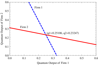
Figure 1: (Color online) The quantity reaction curve for $\gamma=5,r_{1}=0.45,r_{2}=0.75,t=0.2$

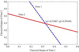
Figure 2: (Color online) The quantity reaction curve for $\gamma=0,r_{1}=0.45,r_{2}=0.75,t=0.2$

Figure 1 shows the equilibrium point for the Firm 1 and Firm 2 in the quantum game for the entanglement operator $\gamma=5$. As expected the classical game is found to be a subset of this quantum structure and our result for $\gamma=0$, shown in Fig. 2, reproduces the classical result given in chap7 . Tables 1 & 2 provide more detailed information on the quantum equilibria of this quantity game. For every table including Tables 1 & 2, the data given in the sub-tables are for firm 1. Transposing these sub-tables gives the corresponding data for firm 2. For example, for the location pair $(r^{i}_{1},r^{j}_{2})$ if the output of firm 1 is $q_{ij}$, then output of firm 2 is $q_{ji}$.

Table 1: Quantum solutions of the game for t=0.2, $\gamma=5$. Data in sub-tables are for firm 1. Transposing these sub-tables gives the corresponding data for firm 2. For example, for the location pair $(r^{i}_{1},r^{j}_{2})$ if the output of firm 1 is $q_{ij}$, then output of firm 2 is $q_{ji}$.

Table 2: Quantum solutions of the game for t=0.6, $\gamma=5$.

Tables 3 & 4 show that setting $\gamma=0$, in our theory we can reproduce the classical game results given in chap7 .

Table 3: Classical(i.e. $\gamma=0$) solutions of the game for t=0.2.

Table 4: Classical(i.e. $\gamma=0$) solutions of the game for t=0.6.

A careful examinations indicate that for any location pair $(r_{1},r_{2}),$ an increase in the transport rate $t$ increase the mill prices, but reduces the quantity produced by each firm and also reduce profits. The results also provide a benchmark against which we can assess the actual locations the firms choose in the location stage of the quantity location game. Independent of the transport rate, when the firms are located symmetrically (i.e. $r_{2}=1-r_{1})$, the individual firm profit is maximised when the firms are located inside but $near$ the quartiles. The aggregate output is maximized when the firms are located symmetrically. But surprisingly, the symmetric location pair that maximises aggregate output is more agglomerated when the transport rate is higher. Low transport costs encourage agglomeration and quantity competition. Higher transport costs imply that sales decline relatively quickly with distance from the firm and so give heavier weight to consumers close to the firm. This moderates somewhat the competitive pressures of proximate locations.

Another intriguing result is expressed in Fig. 3.

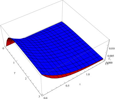
Figure 3: (Color online) The quantum benefit $\Gamma_{i}=\Pi_{i}^{Q}-\Pi_{i}^{C}$ at equilibrium point over the classical equilibrium as a function of the transportation cost ‘t’ and the entanglement parameter ‘$\gamma$’. We have selected the location of the firm 1 $r_{1}=0.3$ and the location of the firm 2 $r_{2}=0.6$. Blue plot: Profit for firm 1 w.r.t. transportation cost ‘t’ and ‘$\gamma$’. Red plot: Profit for firm 2 w.r.t. transportation cost ‘t’ and ‘$\gamma$’.

Figure 3 needs some explanation. It is noted that the quantum benefit of the profit of the firm 2, $\Gamma_{2}=\Pi_{2}^{Q}-\Pi_{2}^{C}$ is greater than $\Gamma_{1}=\Pi_{2}^{Q}-\Pi_{2}^{C}$(quantum benefit of the profit of the firm 1) for higher transport cost, whereas it decreases for lower $t$ and finally the difference $\Gamma_{2}-\Gamma_{1}=0$ for $t=0$ and $\gamma=0$. $\Gamma_{2}\geq\Gamma_{1}$, due to the fact that the location $r_{2}=0.6$ of the firm 2 is towards more central than the location $r_{1}=0.3$ of the firm 1. So there is a strong quantum advantage for firm i if the location of the i-th firm is more central.

The plot of the profits for both the firms with the entanglement parameter $\gamma$, for a fixed transport cost and a set of a fixed location parameters given in Figure 4 explains vividly the quantum benefit over its classical counterpart.

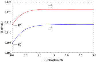
Figure 4: (Color online) Quantum profit at Nash equilibrium w.r.t. the entanglement parameter $\gamma$ for t=0.2, $r_{1}=0.3$ and $r_{2}=0.6$. Blue line: Quantum profit ($\Pi_{1}^{Q}$) of the firm 1 w.r.t. $\gamma$. Red line: Quantum profit($\Pi_{2}^{Q}$) of the firm 2 w.r.t. $\gamma$. Here $\Pi_{i}^{C}$ denoted the classical profit of the i-th firm.

Next, one can analyse the quantum benefit $\Gamma_{i}=\Pi_{i}^{Q}-\Pi_{i}^{C}$ for a fixed $\gamma$ (say, $\gamma=5$) and a fixed set of locations of the firms for different values of the transport cost $t$. The analysis is shown in Fig. 5. The quantum benefit is maximum for zero transport cost for both the firms. As $t$ is increased the benefit rapidly falls for both the firms, but the rate of decrement is more for firm 2 than firm 1 (as we discussed earlier this is also due to the fact that the location of firm 1 is more central also seen in the Fig. 3), and as expected when $t$ attains a much higher value, the quantum benefit $\Gamma_{i}$ asymptotically tends to zero for both the firms, i.e. for a higher transport cost the quantum profit over its classical counterpart is negligible.

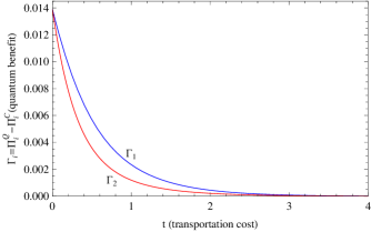
Figure 5: (Color online) The quantum benefit $\Gamma_{i}=\Pi_{i}^{Q}-\Pi_{i}^{C}$ at Nash equilibrium point over the classical Nash equilibrium as a function of the transportation cost ‘t’. Here the entanglement parameter $\gamma=5$, location of the firm 1 $r_{1}=0.3$ and location of the firm 2 $x_{2}=0.6$. Blue line: Quantum benefit($\Gamma_{1}$) for firm 1 w.r.t. transportation cost ‘t’. Red line: Quantum benefit $\Gamma_{2}$ for firm 2 w.r.t. transportation cost ‘t’.

The existence of a symmetric Nash equilibrium (i.e., profit of firm 1= profit of firm 2) for the zero consumer transportation cost is an example of another important feature of this game. We can observe the same feature if $t$ is independent of the distance. The symmetric quantum Nash equilibrium is also obtained if the firms are perfectly agglomerated ($r_{1}=r_{2}$) or symmetrically located ($r_{1}=1-r_{2}$). A key feature in Li. et. al LDM02 is the zero transportation cost or the firms location are perfectly agglomerated and the quantum profit gain at Nash equilibrium over classical is equivalent to the case given in figure 6, where the locations of the firms are considered to be symmetric within the market i.e. $r_{1}=1-r_{2}$.

Figure 6: The profits at quantum Nash equilibrium w.r.t the entanglement parameter $\gamma$, when the two firms are perfectly agglomerated or, symmetric location(i.e. $r_{1}=1-r_{2}$) for t=0.2, $r_{1}0.3$ and $r_{2}=0.7$. Here both the quantum (classical) profits are same, i.e. $\Pi_{1}^{Q}=\Pi_{2}^{Q}$ ($\Pi_{1}^{C}=\Pi_{2}^{C}$).

The quantization of a classical game can be termed as successful when the quantum profit is higher than the classical profit. A critical comparison of the Tables 1, 2, 3 and 4 very nicely explain the competency of our model in this regard by showing that for different transport costs, at equilibrium points, the quantum profit is more than the corresponding classical profit. The behaviour in outputs of the firms for the quantum version of the game is similar to that of its classical counterpart, but with higher profit. Like classical situation, in quantum case there also exists a transport cost $t_{g}^{Q}(\gamma)$ ($\cong 0.39353;$ when, $\gamma=5$) for which, any $t<t_{g}^{Q}(\gamma)$ firm i’s profit is always greater, if the location of the firm is nearer to the market centre. Also,

$$\lim\limits_{r_{1},r_{2}\to 0.5}q_{i}^{Q}(r_{1},r_{2})=[(8-13t)\cos{\gamma}-t\sin{\gamma}+\surd((64+t(80+97t))\cos^{2}{\gamma}$$

$$+t\sin{\gamma}(2(40+t)\cos{\gamma}+t\sin{\gamma}))]/(16(3\cos{\gamma}+\sin{\gamma}))$$ (23)

$$\lim\limits_{r_{1},r_{2}\to 0.5}p_{i}^{Q}(r_{1},r_{2})=[(16+7t)\cos{\gamma}+\sin{\gamma}(8-t)-\surd((64+t(80+97t))\cos^{2}{\gamma}$$

$$+t\sin{\gamma}(2(40+t)\cos{\gamma}+t\sin{\gamma}))]/(8(3\cos{\gamma}+\sin{\gamma}))$$ (24)

IV Game with transport allowance

Finally, in this section we describe a fascinating situation. Let us think of the case when a consumer does not bear the transport cost, instead the consumer earns some amount of money as $transport$ $allowance$ for his/her transportation to the firm for buying any product . This situation can be explored by setting $t$ a negative value, where each consumer earns an amount $u=-t$ per unit distance when they travel to the seller(Firm) to collect the goods. We call it $transport$ $allowance$ and denote it as $u=-t$ per unit distance.

Numerical computations are displayed in the Tables 5 & 6.

Table 5: Classical(i.e., $\gamma=0$) solutions of the game for t=-0.2.

Table 6: Quantum solutions of the game for t=-0.2, $\gamma=5$.

Next, we analyse the variation of the profit with the transport allowance $-t=u$ and entanglement parameter $\gamma$. Figures (7& 8) show the variation of the profit $\Pi_{i}$ (i=1,2) for a wide range of t, ($-1.5<t<1$) and $\gamma$. We denote $t=t_{c}$ as a critical point for the profit of the firm $i$, $\Pi_{i}$, when the profit is zero and after that starts to be negative ( $\Pi_{i}<0$). For any $\Pi_{i}<0~{}(i=1,2)$, it is seen that for $t<t_{c}<0$, at least one optimal profit is negative. We can write $-t_{c}=u_{c}$ as the critical $travel$ $allowance$.

The $t$-$\gamma$ plane with $\Pi_{i}=0$ is denoted as the zero profit plane. It is noticed that for a large region of $\gamma$ and $-ve$ ‘t’, the quantum profit is still above the ‘0’ profit plane (i.e. positive), whereas in the classical case, profit is below the ‘0’ profit plane which means profit is negative.

With this analysis, another important feature of quantum game theory can be explored. Let $SS=\{(q_{1},q_{2},p_{1},p_{2})|0\leq q_{i},p_{i}(i=1,2)\}$ be the Strategic Space(SS) and $OSS$ be the Optimal Strategic Space(OSS) of a quantity equilibrium game for fixed location. Therefore, $OSS\subset SS$.
For $\Pi_{i}=q_{i}p_{i}<0\Rightarrow$ we should have either $p_{i}<0$ or, $q_{i}<0$, i.e., for negative profit the equilibrium strategic point $(q_{1},q_{2},p_{1},p_{2})\notin SS(\supset OSS)$.

Figures (7& 8) show that for both the firms $t_{c}^{Q}<t_{c}^{C}<0$ for a fixed location ($r_{1}\&r_{2}$), here $-t_{c}^{Q}$ is the genuine($\gamma>0$) quantum critical $travel$ $allowance$ $u_{c}^{Q}$, and $u_{c}^{C}=-t_{c}^{C}$ is the classical critical $transport$ $allowance$. Therefore, $\exists~{}~{}t(<t_{c}^{C}<0)$, such that both the quantum profits $\Pi_{1}^{Q}\&\Pi_{2}^{Q}>0$, whereas at least one classical profit (either $\Pi_{1}$ or, $\Pi_{2}$) is negative, for a fixed location. So the optimal quantum strategic space($OSS^{Q}$) is always larger than the optimal classical strategic space ($OSS^{C}$), which is another feature of importance in a quantum game.

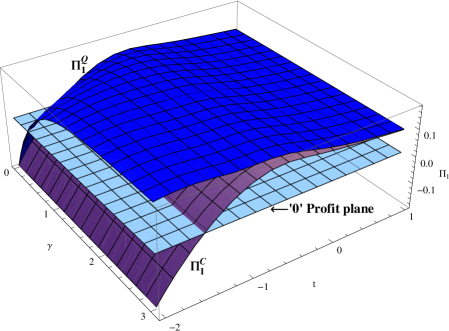
Figure 7: (Color online) Plot of quantum (blue surface) and classical (pink surface) profits with respect to $\gamma$ and t for the location $r_{1}=0.3$ and $r_{2}=0.6$ of firm 1 at equilibrium point. Plot shows that for a large region of $\gamma$ and $negative$ ‘t’, the quantum profit is still above(i.e. positive) the ‘0’ profit plane (cyan surface) , whereas classical profit is negative (i.e. below the ‘0’ profit plane).

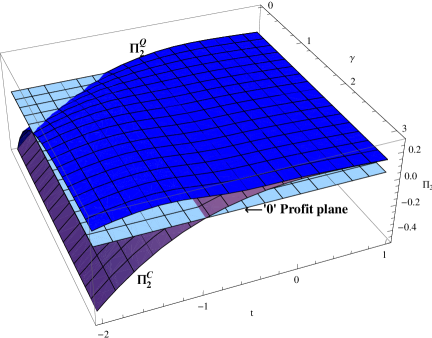
Figure 8: (Color online) Plot of quantum (blue surface) and classical (pink surface) profits with respect to $\gamma$ and t for the location $r_{1}=0.3$ and $r_{2}=0.6$ of firm 2 at equilibrium point. Plot shows that for a large region of $\gamma$ and $negative$ ‘t’, the quantum profit is still above(i.e. positive) the ‘0’ profit plane (cyan surface) , whereas classical profit is negative (i.e. below the ‘0’ profit plane).

The plots (7 & 8) and the tables (5 & 6) indicate that if the present two-stage game is played, either classically or in the quantum domain, with transport allowance instead of transportation cost then:
For any location pair $(r_{1},r_{2})$ if firm 1 is located nearer the market centre than firm 2, then

• firm i produces a greater output than firm k:
  $q_{1}^{c}(r_{1},r_{2})\gtreqless q_{2}^{c}(r_{1},r_{2})$ if $r_{1}\lesseqgtr 1-r_{2}$;

• firm i will charge a higher mill price than firm k:
  $p_{1}^{c}(r_{1},r_{2})\gtreqless p_{2}^{c}(r_{1},r_{2})$ if $r_{1}\lesseqgtr 1-r_{2}$; and

• firm i will earn greater profit than firm k:
  $\Pi_{1}^{c}(r_{1},r_{2})\lesseqgtr\Pi_{2}^{c}(r_{1},r_{2})$ if $r_{1}\gtreqless 1-r_{2}$

which implies that for negative ‘t’, there is a strong competitive advantage when the firm location are nearer the end of the market boundary unlike the case when the transport cost ‘t’ is positive.

V Conclusion

In this Letter, we explore some interesting cases of Hotelling-Smithies model of product choice where the player can be benefited more by adopting a quantum strategy rather the classical strategy, leaving a large number of cases unresolved. Specially, the quantum benefit in Bertrand competition (with transport cost indiscrimination) which seems a more difficult problem than the case of Cournot quantity competition. We also demonstrate the fact that the quantum equilibrium strategic space of a Cournot quantity competition game is larger than the classical equilibrium strategic space. Although, this result as expected, is uncommon for any quantum game having only linear demand function and hope that this result would encourage the researchers in this area to develop the field further.

VI acknowledgments

The authors acknowledge helpful discussions with Dr. Kausik Gangopadhyay. R.R. also acknowledges support from Norwegian Research Council.

References

- (1) D.A. Meyer, Phys. Rev. Lett. 82 (1999) 1052.
- (2) J. Eisert, M. Wilkens, and M. Lewenstein, Phys. Rev. Lett. 83, 3077 (1999).
- (3) S.C. Benjamin and P.M. Hayden, Phys. Rev. A 64, 030301 (2001).
- (4) H. Li, J. Du and, Se. Massar, Phys. Lett. A, 306, 73-78(2002).
- (5) C. D. Hill, A. P. Flitney, N. C. Menicucci, Phys. Lett. A 374 (2010) 3619-3624.
- (6) R. Prevedel, A. Stefanov, P. Walther and A. Zeilinger, New J. of Phys. 9 (2007) 205.
- (7) C. Schmid, A. P. Flitney, W. Wieczorek, N. Kiesel, H. Weinfurter and L. C. L. Hollenberg, New J. of Physics 12 (2010) 063031.
- (8) J. Du, H. Li, X. Xu, M. Shi, J. Wu, X. Zhou, and R. Han, Phys. Rev. Lett. 88, 137902 (2002).
- (9) P. Ball, Economics Nobel 2001, Sceince Update, 16 Oct. 2001
- (10) Harold Hotelling, The Economic Journal, 39, 41-57 (1929).
- (11) A. Smithies, Journal of Political Economy 49, 423-439 (1941).
- (12) Ali Al-Nowaihi, G. Norman, Market evolution: competition and cooperation (European Association for Research in Industrial Economics, Conference- Business and Economics), Kluwer Academic Publishers 1995, Chapter 7, Page 101-127.
- (13) S.L. Braunstein, H.J. Kimble, Phys. Rev. Lett. 80 (1998) 869.
- (14) A. Furusawa, J. L. Srensen, S. L. Braunstein, C. A. Fuchs, H. J. Kimble and E. S. Polzik, Science 282 (1998) 706.
- (15) G.J. Milburn, S.L. Braunstein, Phys. Rev. A 60 (1999) 937.
- (16) C.F. Lo, D. Kiang, Phys. Lett. A 318, 333 (2003); C.F. Lo, D. Kiang, Phys. Lett. A 346, 65 (2005).