DESY 12-023
DO-TH 11/31
LPN 12-033
SFB/CPP-12-08
February 2012
Parton distribution functions and benchmark cross sections
at NNLO
S. Alekhin111e-mail: sergey.alekhin@ihep.ru,
J. Blümlein222e-mail: johannes.bluemlein@desy.de,
and S. Moch333e-mail: sven-olaf.moch@desy.de
aDeutsches Elektronensynchrotron DESY
Platanenallee 6, D–15738 Zeuthen, Germany
bInstitute for High Energy Physics
142281 Protvino, Moscow region, Russia
Abstract
We present a determination of parton distribution functions (ABM11) and the strong coupling constant at next-to-leading order and next-to-next-to-leading order (NNLO) in QCD based on world data for deep-inelastic scattering and fixed-target data for the Drell-Yan process. The analysis is performed in the fixed-flavor number scheme for and uses the -scheme for and the heavy-quark masses. At NNLO we obtain the value . The fit results are used to compute benchmark cross sections at hadron colliders to NNLO accuracy and to compare to data from the LHC.
1 Introduction
Parton distribution functions (PDFs) in the nucleon are an indispensable ingredient of modern collider phenomenology and their study has a long history. In the perturbative approach to the gauge theory of the strong interactions, Quantum Chromodynamics (QCD), factorization allows for the computation of the hard parton scattering processes as a power series in the strong coupling constant and, typically, to leading power dominating for large momentum transfer . Predictions for physical cross sections involving initial hadrons, however, do require further non-perturbative information, that is knowledge of the PDFs in the nucleon as well as the value of and of the masses of heavy quarks. Since PDFs cannot be calculated in perturbative QCD, they need to be extracted from a comparison of theory predictions to available experimental precision data on deep-inelastic scattering (DIS), on the production of lepton-pairs (Drell-Yan process) or jets in hadron collisions or any other suitable hard scattering reaction.
The accuracy of PDF determinations in such analyses has steadily improved over the years, both due to more accurate experimental input and due to refined theory predictions for the hard parton scattering reactions including higher orders in perturbation theory. As of now, complete next-to-next-to-leading order (NNLO) calculations in perturbative QCD form the backbone of this endeavor. These allow for the computation of many important benchmark cross sections, e.g. in the proton-proton collisions at the LHC, with an unprecedented precision. The determination of PDFs to NNLO accuracy in QCD was pioneered more than a decade ago in [1] and builds in particular on the known corrections for the PDF evolution [2, 3] as well as on the hard scattering corrections for DIS [4, 5, 6, 7, 8, 9, 10], and hadronic - and -gauge-boson production, both at an inclusive [11, 12] and a differential level [13, 14, 15].
Presently, NNLO PDFs have been obtained by a number of different groups. In detail, these are ABKM09 [16, 17], HERAPDF1.5 [18, 19], JR09 [20, 21], MSTW [22] and NN21 [23], while CT10 [24] still remains at next-to-leading order (NLO) accuracy only. There exist, of course, differences between these PDF sets. These arise from variations in the choice of the parameters, e.g., the value of , but also from a different theoretical footing for the data analysis. In the latter case, this comprises for instance, the treatment of the heavy-quark contributions in DIS, the corrections for nuclear effects, the inclusion of higher twist (HT) terms and so on. The implications for precision predictions at TeV-scale hadron colliders can be profound, though, as benchmark cross sections at NNLO in QCD for the production of - and -gauge-bosons or the Higgs boson through gluon-gluon-fusion (ggF) show, see e.g., the recent discussion in [25, 26, 27, 28, 29, 30].
In this article we present the PDF set ABM11, which is an updated version of the PDF analyses of ABKM09 [16] and ABM10 [17] in the 3-, 4-, and 5-flavor scheme at NNLO in QCD. These PDFs are obtained from an analysis of the world DIS data combined with fixed-target data for the Drell-Yan (DY) process and for di-muon production in neutrino-nucleon DIS. In the ABM11 fit we are now using the final version of the DIS inclusive data collected by the HERA experiments in run I [18] together with new data of the H1 collaboration from the HERA low-energy run [31]. Moreover, our update is based on theoretical improvements. For instance, the treatment of the heavy-quark contributions in DIS now employs the running-mass definition in the -scheme for the heavy quarks [32].
The strong coupling constant or, respectively, the QCD scale , is a mandatory parameter to be fitted in DIS analyses of world data, its correct value being of paramount importance for many processes in DIS and at hadron colliders, in particular for Higgs boson production in ggF [26]. An essential criterion for the selection of additional precision data on top of the world DIS data, e.g. those for the DY process or for hadronic weak-boson and jet-production cross sections, in the measurement of the QCD scale is the compatibility of these data sets with respect to the experimental systematics in the different measurements. Strictly speaking, combined analyses require a theoretical description at the same perturbative order. Because of these reasons, the combination of different data sets needs great care if performed with the goal of a precision measurement of . Combinations of a wide range of hard-scattering data sets of differing quality, as sometimes used in more global fits, are useful only, if they indeed lead to a statistically and systematically improved value of . Of course, a careful check is always required when new data sets are added. As a result of our new analysis we determine in the ABM11 fit the strong coupling constant at NNLO in the -scheme and present a detailed discussion of the uncertainties and of the impact of individual experiments, showing the great stability in the obtained value of .
The papers is organized as follows. In Sec. 2 we describe the theoretical framework of our analysis, in Sec. 2.1 in particular the perturbative QCD input including the framework for heavy-quark DIS. Secs. 2.2 and 2.3 are concerned with a detailed account of the non-perturbative corrections and nuclear corrections, which have already been applied in previous PDF analyses [16, 17]. Sec. 3 features in detail the data analysed with an emphasis on the systematic and normalization uncertainties. This comprises data on inclusive DIS from the HERA collider and fixed target experiments in Sec. 3.1, on the DY process in Sec. 3.2 and on di-muon production in neutrino-nucleon DIS in Sec. 3.3.
The main results of the present work are contained in Sec. 4, where we present all PDF parameters along with illustrations of the shapes of PDFs. The numerous checks include studies of the pulls and the statistical quality for all individual experiments as well as a detailed assessment of the power corrections induced by the higher twist terms. As we work in a scheme with a fixed number of light quark flavors, a detailed discussion is also devoted to the generation of heavy-quark PDFs. Our determination of the strong coupling constant at NNLO in QCD leads to the value . We show the impact of the individual data sets on and compare with the determinations from other PDF fits and other measurements included in the current world average. Finally, Sec. 4 is complemented with a comparison of moments of PDFs with recent lattice results.
The consequences of the new PDF set ABM11 on standard candle cross section benchmarks are illustrated in Sec. 5. We provide cross section values for - and -boson production in schemes with and flavors and we address the accuracy of theory predictions for all dominant Higgs boson search channels at the LHC. The PDF uncertainties for top-quark pair-production are also illustrated highlighting the combined uncertainty in the gluon PDF, and the top-quark mass . Sec. 5 finishes with comments on the issue of hadronic jet production, especially from the Tevatron, and the impact of its data on PDF fits. We conclude in Sec. 6 and summarize our approach for the handling of the correlated systematic and normalization uncertainties along with the explicit tables for the covariance matrix of the ABM11 fit in App. A.
2 Theoretical framework
Here, we briefly recall the theoretical basis of our PDF analysis, which is conducted in the so-called fixed-flavor number scheme (FFNS) for light (massless) quarks. That is to say, we consider QCD with light quarks in the PDF evolution, while heavy (massive) quarks only appear in the final state. As far as QCD perturbation theory is concerned, we specifically focus on aspects relevant to NNLO accuracy. For completeness our treatment of power corrections and also of nuclear corrections as needed e.g., for DIS from fixed-target experiments, is documented in Sec. 2.2 and 2.3. The latter have already been used in our previous PDF determinations [16, 17].
2.1 Perturbative QCD
The ability to make quantitative predictions in QCD which is a strongly coupled gauge theory, rests entirely on its factorization property. A cross section for the production of some final state from scattering of initial state hadrons can be expressed in lepton-nucleon () DIS as,
| (2.1) |
for and in proton-proton collisions () as,
| (2.2) | |||||
where the PDFs in the nucleon () are the objects of our primary interest. They describe the nucleon momentum fraction (or , ) carried by the parton and the sums in eqs. (2.1) and (2.2) run over all light (anti-)quarks and the gluon. The parton cross sections denoted are calculable in perturbation theory in powers of the strong coupling constant and describe the hard interactions at short distances of order . We have also displayed all implicit and explicit dependence on the renormalization and factorization scales, and . Throughout our analysis, however, we will identify them, . All dependencies of and on the kinematics and, likewise the integration boundaries of the convolutions, has been suppressed in eqs. (2.1) and (2.2), as these are specific to the observable under consideration.
In standard DIS, the (semi-)inclusive cross section in eq. (2.1) depends on the Bjorken variable , the inelasticity and on , the (space-like) momentum-transfer between the scattered lepton and the nucleon. Moreover, it admits a decomposition in terms of the well-known DIS (unpolarized) structure functions , . QCD factorization applied to the DIS structure functions implies
| (2.3) |
where , , , and denote the Wilson coefficients. defines the longitudinal structure function in terms of the tranverse structure function , see also eq. (3.2) below for the relation including target masses. Eq. (2.3) integrated over gives rise to the standard Mellin moments,
| (2.4) |
These link the theoretical description of DIS to the operator-product expansion (OPE) on the light-cone. The OPE allows to express the DIS structure functions as a product of (Mellin moments of) the Wilson coefficients and operator matrix elements (OMEs) of leading twist (twist-2). Moreover, it admits a well-defined extension in powers of (twist-4, twist-6 and so on), cf. Sec. 2.2.
The scale dependence of the PDFs is contained in the well-known evolution equations
| (2.5) |
at leading twist, which is a system of coupled integro-differential equations corresponding to the different possible parton splittings. The splitting functions in eq. (2.5) have been determined at NNLO in [2, 3], which implies knowledge on the first three terms in the powers series in (suppressing parton indices),
| (2.6) |
The PDFs are subject to sum rule constraints due to conservation of the quark number and the momentum in the nucleon, which imply at each order in perturbation theory a vanishing first (second) Mellin moment for specific (combinations of) splitting functions in eq. (2.6). These sum rule constraints relate the PDF fit parameters used in the parametrizations of the input distributions, see Sec. 4. The accuracy of the numerical solution of the differential eq. (2.5) up to NNLO was tested by comparison to programs such as QCD-PEGASUS [33] or HOPPET [34].
For the massless DIS structure functions we will be using the following input from perturbative QCD at leading twist,
| (2.7) |
where, again, (NLO) NNLO accuracy is defined by the first (two) three terms in the power series in , cf. eq. (2.6). The Wilson coefficients for , in eq. (2.7) are known to NNLO from [4, 5, 6, 7, 8], and, actually, even to next-to-next-to-next-to-leading order (N3LO) from [10, 35], and for to NNLO from [9, 10]. Note that in the latter case the perturbative expansion starts at order , thus NNLO accuracy for actually requires three-loop information, which is numerically not unimportant.
Likewise, for the partonic cross sections of the DY process in eq. (2.2), i.e., for hadronic - and -boson production, we use
| (2.8) |
At the level of NNLO accuracy, QCD perturbation theory is expected to provide precise predictions as generally indicated by the numerical size of the radiative corrections at successive higher orders and their pattern of apparent convergence. The residual theoretical uncertainty from the truncation of the perturbative expansion is conventionally estimated by studying the scale stability of the prediction, i.e., by variation of the renormalization and factorization scales and in eqs. (2.1) and (2.2). As stated above, we set in our analysis, and moreover, identify the scale with the relevant kinematics of the process, e.g., for DIS. Currently no PDF fits with an independent variation of and are available and we leave this issue for future studies.
One important aspect is the production of heavy quarks in DIS both for the neutral-current (NC) and the charged-current (CC) exchange. In the former case, pair-production of charm-quarks accounts for a considerable part of the inclusive DIS cross section measured at HERA, especially at small Bjorken-, while the latter case is needed in the description of neutrino-nucleon DIS. At not too large values of , the NC reaction is dominated by the photon-gluon fusion process , while the CC case proceeds through , so that the perturbative expansion of the respective heavy-quark structure functions reads,
| (2.9) |
where and is the heavy-quark mass. The heavy-quark Wilson coefficients are known exactly to NLO, both for NC [36] and CC [37, 38]. The NNLO results for are, at present, approximate only and based on the logarithmically enhanced terms near threshold [39, 40, 41] (see [42] for threshold resummation in the CC case). As well known [43], the heavy-flavor corrections to are represented with an accuracy of and better for . Under this condition the Wilson coefficients are given by Mellin convolutions of massive OMEs [43, 44, 45, 46] and the massless Wilson coefficients [4, 5, 6, 7, 8, 9, 10]. Fixed Mellin moments of the heavy-quark OMEs have also been computed at three loops in [47] and first results for general values of Mellin- have been calculated in [48]. Mellin space expressions for the NC and CC Wilson coefficients up to are available in [49, 50].
In the current PDF analysis, the bulk of data from DIS experiments can be described in a scheme with light flavors. At asymptotically large scales the genuine contributions for heavy charm- and bottom-quarks in a FFNS with grow as , as the quark masses screen the collinear divergence. The standard PDF evolution equations in eq. (2.5) resum these logarithms at the expense of matching the effective theories, i.e. QCD with and light flavors. This defines a variable-flavor number scheme (VFNS) and gives rise to the so-called heavy-quark PDFs for charm- and bottom-quarks in QCD with effectively and light flavors. The heavy-quark PDFs are generated from the light flavor PDFs in a -flavor FFNS as convolutions with OMEs, see e.g. [44, 16]. The VFNS requires the matching conditions both for the strong coupling and the PDFs (through the corresponding OMEs), which are known to N3LO [51, 52] for and to NNLO for the OMEs [44, 46]. An extensive discussion of the VFNS implementation has been presented in our previous analysis [16].
The heavy-quark masses in eq. (2.9) are well-defined within a specific renormalization scheme, the most popular ones being the on-shell and the -scheme. The former uses the so-called pole-mass , defined to coincide with the pole of the heavy-quark propagator at each order in perturbative QCD, and known to have intrinsic theoretical limitations. As a novelty of our analysis, we employ the -scheme for , which enters both in the massive OMEs and in the Wilson coefficients and introduces a running mass depending on the scale of the hard scattering in complete analogy to the running coupling . As a benefit, predictions for the heavy-quark structure functions in terms of the -mass display better convergence properties and greater perturbative stability at higher orders [32], thus reducing the inherent theoretical uncertainty.
The Fortran code OPENQCDRAD for the numerical computation of all hard scattering cross sections within the present PDF analysis is publicly available [53]. It comprises in particular the theory predictions for the DIS structure functions including the heavy-quark contributions as well as for the hadronic - and -boson production and it is capable of computing of the benchmark cross sections to NNLO accuracy in QCD in Sec. 5.
We neglect all effects due to Quantum Electrodynamics (QED) on the PDF evolution. For reasons of consistency, QED effects (including a photon PDF, see e.g., the analysis in see [54]) are sometimes needed in computations of cross sections including electroweak corrections at higher orders. Quite generally the effects are small, though. The NNLO QCD corrections to the photon’s parton structure are known [55, 56] and we will address this issue in a future publication.
2.2 Power corrections
The leading twist approximation to the QCD improved parton model is valid only at asymptotically large momentum transfers and the factorization underlying eqs. (2.1) and (2.2) is not sensitive to the finite hadron size effects or, equivalently, to soft hadronic scales like the nucleon mass . At low momentum transfer comparable to the nucleon mass such hadronic effects cannot be ignored and the standard factorization ansatz acquires power corrections in . In the case of PDF analyses the higher twist terms are especially important for the DIS data since they cover a kinematical range down to . The power corrections for the kinematics of DY data used in our fit (cf. Sec. 3) are negligible due to the large momentum transfer in this case. Therefore we do not consider power corrections for the DY process.
In DIS the power corrections arise from kinematic considerations once the hadron mass effects are taken into account, i.e., the so-called target mass correction (TMC). The TMC can be calculated in a straightforward way from the leading twist PDFs within the OPE [57]. In our analysis the TMC are taken into account in the form of the Georgi-Politzer prescription [57]. For relevant observables, i.e., the structure function and the transverse one it reads
| (2.10) |
and
| (2.11) |
respectively, which holds up to . Here and is the Nachtmann variable [58]. The quantities on the right hand side of eqs. (2.10) and (2.11) are the leading twist structure functions introduced in eq. (2.7) above.
Power corrections can also arise dynamically as so-called higher twist terms from correlations of the partons inside the hadron. The twist-4 terms in the nucleon structure function turns out to be non-negligible at large [59, 60]. Moreover, the higher twist terms in the longitudinal structure function appear to be necessary for the description of the NMC data at moderate [27, 61] and the SLAC data on the structure function [62], where and are the absorption cross sections for the longitudinally and the transversely polarized virtual photons, respectively (see also eq. 3.2). The OPE, for lepton-nucleon DIS provides the framework for the systematic classification of the higher twist terms referring to local composite operators of twist-4 and higher [63]. Nonetheless the shapes of the higher twist terms are poorly known. Therefore they cannot be accounted for on the same solid theoretical footing as the leading twist contributions discussed in Sec. 2.1. Furthermore, both, the scaling violations and the Wilson coefficients for the various higher twist contributions have not been computed to the same order in perturbation theory as for the leading twist part.
Basically two strategies exist to address the issue of power corrections in the PDF analysis. The first one imposes kinematical cuts on the data. For DIS, these cuts are performed at high hadronic invariant masses where the nucleon mass is included in the kinematical considerations. In this way, one aims at a data sample with reduced sensitivity to power corrections. Typical values for cuts on are of the order of GeV2. As a drawback of this procedure one eliminates a rather large fraction of data at low with excellent statistical precision. A more serious concern, however, is due to the generally poor theoretical understanding of those non-perturbative QCD effects beyond leading twist factorization. One simply cannot estimate from first principles the region of (or ), where power corrections can be safely neglected. Therefore, the present analysis (following [64]) examines both, TMC and higher twist contributions, in detail in order to control and quantify their impact in the determination of the standard leading twist PDFs.
In practice higher twist contributions are usually parameterized independently from the leading twist one with some function of , which is typically polynomial in . In our analysis the power corrections are non-negligible for the case of the DIS data and are defined within an entirely phenomenologically motivated ansatz, as follows
| (2.12) |
where are given by eqs. (2.10) and (2.11). The coefficients are parameterized by a cubic spline with the spline nodes selected at x=0, 0.1, 0.3, 0.5, 0.7, 0.9, and 1. This choice provides sufficient flexibility of the coefficients with respect to the data analysed and, at the same time, keeps a reasonable number of nodes. The values of are fixed at zero due to kinematic constraints. The values of are also put to zero in view of the fact that no clear signs of any power-like terms can be found in the low- HERA data. The rest of the spline-node values of were fitted to the data simultaneously with the PDF parameters and the value of . We neglect the -dependence of the higher twist operators due to the QCD evolution. Therefore the coefficients do not depend on . This treatment could be further refined by considering the individual (quasi-)partonic OMEs along with their renormalization, i.e., their -dependence, which is known for the twist-4 operators to first order in [65]. Another complication is the emergence of more Bjorken-like variables , the number of which grows with increasing twist. Experimental information on the other hand is only available for the variable and . We leave these aspects for future studies.
With the kinematical cuts imposed on the DIS data in our analysis (cf. Sec. 3) the twist-6 terms are irrelevant [66] therefore the coefficients in eq. (2.12) are washed out. The target dependence of the higher twist parametrization in eq. (2.12) has been studied in [67, 68, 69]. The isospin asymmetry in is poorly constrained by the data used in our fit. It is comparable with zero within the uncertainties [67] and therefore it was put to zero in our analysis. The isospin asymmetry in is also numerically small, however, due to lower uncertainties it cannot be put to zero without deterioration of the fit quality. In summary, we fit three twist-4 coefficients, for the proton , for the neutron and for the nucleon , in addition to the leading twist terms. The impact of the power corrections on the DIS neutrino-nucleon di-muon production data used in our fit is marginal [68] as well as on the inclusive charge-current data [18]. Therefore they are not considered for the case of charged-current structure functions.
2.3 Corrections for nuclear effects
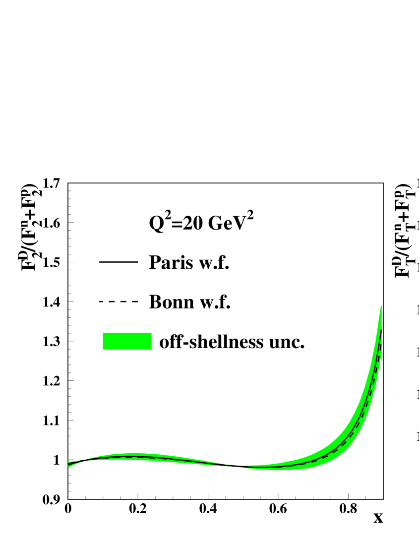
For our analysis we select primarily the data obtained off proton targets. However in some cases the necessary constraints on PDFs come only from nuclear target data. For example the neutral-current DIS off deuterium targets allows the separation of the large- - and -quark distributions, which contribute to the DIS structure functions in the form of linear combination weighted with the quark charges. However the analysis of the deuterium data requires modeling of nuclear effects. They include the Fermi-motion and off-shellness of the nucleons, excess of pions in the nuclear matter, Glauber shadowing, etc., cf. [70, 71] for reviews. Among them only the Fermi-motion effects can be calculated with an uncertainty better or comparable to the uncertainty in the existing experimental data. The Fermi-motion correction is given as a convolution of the free nucleon structure functions with the deuterium wave function, which in turn is constrained by the low-energy electron-nuclei scattering data. The parameterization of the off-shell effect used in our fit was obtained from the analysis of the world data on DIS off heavy nuclear targets and extrapolated to the deuterium target. In this way we assume that the nuclear model suggested in [70] can be applied to the case of light nuclei, like deuterium. This assumption has been recently confirmed for the case of the and targets [72]. However, in order to take a conservative estimate of the deuteron correction uncertainty due to the off-shellness effect we vary its magnitude by 50%. The uncertainty obtained in this way is comparable with one given in [71]. Other nuclear effects, like shadowing and pion excesses in nuclei considered in [70] were found numerically negligible for the case of deuterium. Thus our model of the nuclear effects for deuterium is based on the combination of the Fermi-motion and the off-shellness effects only. The nuclear corrections depend both on the deuterium wave function and the free nucleon structure functions, while the latter include the target-mass corrections and the twist-4 terms, cf. eq. (2.12). Due to the structure function dependence the value of the correction is sensitive to the fitted parameters and ideally it should be re-calculated iteratively in the fit. However, this approach turns out to be rather time-consuming. Therefore we calculate the deuteron correction once at the beginning with the PDFs and twist-4 terms which were obtained in [16]. Since the deuteron model employed in our fit is the same as one of [16] this approach introduces only a marginal bias into the fit. The nuclear correction for the representative kinematics of the deuterium data is given in Fig. 2.1 for the cases of the deuterium wave function obtained with the Paris potential of [73] used in our analysis and the Bonn potential of [74]. The difference between these two cases is marginal as compared to the errors in the data. The data on di-muon production in the (anti-)neutrino-nucleon scattering which are used in our analysis in order to constrain the strange sea distribution, were obtained on iron targets. In contrary to the neutral-current case a particular shape of the nuclear correction at large is unimportant since data do not populate the region of . At small the neutrino-nucleon DIS nuclear corrections are enhanced due to the parity non-conserving part of the charged current [75], however their impact on the strange sea distribution is still smaller than its error [68]. Therefore in the modeling of the di-muon production data we employ the nuclear corrections of [75] without consideration of their uncertainties. The DY data used in our fit span the moderate- region. For such kinematics the nuclear effects are quite smaller than the errors in data [76] and they are not considered in our analysis.
3 Data
The nucleon PDFs are usually extracted from a combination of hard-scattering data, which provides complementary constraints on the different PDF species. A particular choice of which processes to be used in an analysis is commonly driven by the theoretical accuracy of the data modeling and/or the experimental uncertainties in the data. In our fit we employ the data on inclusive DIS, the DY process, and di-muon production in neutrino-nucleon DIS. In combination they allow for a good separation of the quark flavors in wide range of and provide good constraints on the gluon distribution at small values of , which are mostly important for the collider phenomenology.
3.1 Inclusive DIS
Studies of inclusive DIS date back to the early days of QCD and since that time a wealth of the accurate data has been collected. The first fixed-target DIS experiments at SLAC were followed by data from CERN and Fermilab and then at the electron-proton collider HERA at DESY. The most accurate data of these experiments obtained on the proton and deuterium targets are included into our analysis [77, 78, 79, 80, 81, 82, 83, 84, 31].
In all cases we employ the data on the inclusive cross section, which is related to the DIS structure functions as follows
| (3.1) | |||||
with the mass of the incident charged lepton and corresponding to different polarizations for the case of the charged current. The nucleon structure functions , and are calculated with account of the nuclear correction described in Sec. 2.3, if relevant. Note, that higher twist contributions to are set to zero, cf. Sec. 2.2. In this way we provide a consistent treatment of the data, contrary to the common procedure in global PDF fits which are based on the data for the structure function . The structure functions and in eq. (3.1) also enter in the ratio of the longitudinally to transversely polarized virtual photon absorption cross sections (see e.g. [85]),
| (3.2) |
In order to avoid contributions from nucleon resonances and the twist-6 terms we do not include into the analysis any inclusive DIS data with
| (3.3) |
The kinematics spanned by each DIS data set used in our fit and their systematic uncertainties are described in the following subsections. The normalization uncertainty is a particular case of the systematics. However it is considered separately since very often the absolute normalization of the DIS experiment is not independently determined. Instead, in such cases it is usually tuned to a selected set of other DIS experiments, which in turn provide the absolute normalization. The wealth of the DIS data used in our fit allows us to extend the basis for this normalization tuning. Therefore, for the experiments lacking an absolute normalization we consider general normalization factors which are fitted simultaneously with other parameters of our data model. Within this approach we introduce free normalization parameters for the separate early SLAC experiments of [77, 78, 79, 80] and for the NMC data of [84] at each beam energy. The errors in the normalization factors obtained in our fit are included into the general covariance matrix calculation. In this way we account for the impact of the absolute normalization uncertainty in the data on the PDFs, the higher twist terms and on the value of .
Our procedure for the treatment of the DIS data normalization in PDF fits differs substantially from other approaches. For instance, in the MSTW PDF fit [22] free normalization parameters are introduced for all data sets, including even those where the absolute normalization has been determined experimentally. Other PDF fits also commonly employ the NMC data averaged over the beam energies and combined data from the SLAC experiments, rather than the respective individual data sets.
3.1.1 HERA
In our analysis we use the HERA data on the inclusive neutral-current and the charged-current cross sections [18]. This sample was obtained by a combination of the run I data of the H1 and ZEUS experiments, and includes in particular the data of [86, 87] used earlier in the ABKM09 fit [16]. The HERA data span the region of up to . However, we impose an additional cut of on the neutral-current sample. This allows to neglect the -boson exchange contribution, which is of the order at . At the same time, the high- part of those data displays only a poor sensitivity to our PDF fit, since the accuracy of those HERA data is . Therefore the chosen cut does not distort the fit in any way. The normalization uncertainty in the HERA data of [18] is 0.5%, much better than one in the HERA data of [86, 87]. In particular due to the improvement in normalization the new data of [18] somewhat overshoot the previous H1 data of [86]. The total number of correlated systematic uncertainties in the HERA data of [18] is 114, including the uncertainties due to the combination procedure and the general normalization. Many of them are improved as compared to the separate experiment samples as a results of cross-calibration in the process of combination.
A complementary set of the inclusive HERA data was obtained by the H1 collaboration in the run with a reduced collision energy [31]. These data are particularly sensitive to the structure function and thereby to the small- shape of the gluon distribution. The normalization uncertainty in the low-energy data of [31] is 3%. The point-to-point correlated systematic uncertainties come from 8 independent sources and there is also a number of uncorrelated systematic uncertainties in the data.
3.1.2 BCDMS
The BCDMS data of [82, 83] used in our fit were collected at the CERN muon beam at energies of 100, 120, 200, and 280 GeV for the incident muons. Due to the use of both proton and deuterium targets in the same experiment these data facilitate flavor separation of PDFs at large . The BCDMS absolute normalization was monitored for the beam energy of 200 GeV. The general normalization uncertainty in the data due to this monitor is as big as 3%. The absolute normalization of the data obtained at the beam energies of 100, 120, and 280 GeV was calibrated with respect to the case of the beam energy setting of 200 GeV. The additional normalization uncertainty due to this calibration ranges from 1% to 1.5% depending on the beam energy. Other systematic uncertainties in the BCDMS data stem from 5 sources with the most important contributions due to incident and scattered muon energy calibration and the spectrometer resolution. Every source generates a point-to-point correlated uncertainty in the data, while the sources itself are uncorrelated with each other.
3.1.3 NMC
The NMC experiment was performed like BCDMS at the CERN muon beam at incident muon energies of 90, 120, 200, and 280 GeV. However, the NMC data span lower values of and as compared to BCDMS and overlap with the HERA data at the edge of the respective kinematics. We use in our fit the NMC cross section data of [84] for the proton and deuterium targets. Due to better coverage of the small- region those data are also sensitive to the isospin asymmetry in the sea distribution. The absolute normalization for the NMC data of [84] was determined from tuning for each particular energy setting separately to the BCDMS and SLAC data, which overlap partially with NMC. This tuning in [84] was based on an empirical data model motivated basically by leading-order QCD calculations.
In our analysis, therefore, we fit the NMC normalization factors for each incident beam energy and target simultaneously with the other parameters. In this manner, we ensure consistency with our data model, which in particular includes QCD corrections up to the NNLO, see [27] for a detailed study of the impact of the NNLO QCD corrections on the interpretation of the NMC data. The normalization factors obtained in the NNLO variant of our fit are given in Tab. 3.1. In general they are within the uncertainty of 2% quoted for the NMC data in [88]. However, the normalization factors for the proton target are somewhat larger than for the case of deuterium. This is explained by impact of the HERA data of [18], which slightly overshoot the NMC data in the region of their overlap. The systematic uncertainties in the NMC data are due to the incident and scattered muon energy calibration, the reconstruction efficiency, acceptance, and the electroweak radiative corrections. Some of the systematic uncertainties are correlated for all data, some of them between the proton and deuterium data, and some between beam energies (cf. [84] for details). In summary this gives 12 independent sources of systematic uncertainties for the NMC data used in our fit.
| Beam energy (GeV) | proton | deuterium |
|---|---|---|
| 90 | 1.012(12) | 0.990(12) |
| 120 | 1.026(11) | 1.005(11) |
| 200 | 1.034(12) | 1.014(11) |
| 280 | 1.026(11) | 1.007(11) |
3.1.4 SLAC
The SLAC experiments used in our fit and the number of data points for each experiment after the cut of eq. (3.3) are listed in Tab. 3.2. The last and most elaborated in this series is experiment E-140 [81]. In particular, it took advantages of the improved electroweak radiative corrections and the accurate determination of the data absolute normalization, which is as big as 1.8% for the deuterium sample. Other point-to-point correlated systematic uncertainties are due to background contamination, the spectrometer acceptance, and the electroweak radiative corrections [89]. The rest of systematic error sources for the experiment E-140 are uncorrelated.
| Experiment | Target | NDP | NSE | Normalization | Normalization |
| (our fit) | (Ref. [62]) | ||||
| E-49a [77] | proton | 59 | 3 | 1.012 | |
| deuterium | 59 | 3 | 1.001 | ||
| E-49b [77] | proton | 154 | 3 | 0.981 | |
| deuterium | 145 | 3 | 0.981 | ||
| E-87 [77] | proton | 109 | 3 | 0.982 | |
| deuterium | 109 | 3 | 0.986 | ||
| E-89a [78] | proton | 77 | 4 | 0.989 | |
| deuterium | 71 | 5 | 0.985 | ||
| E-89b [79] | proton | 90 | 3 | 0.953 | |
| deuterium | 72 | 3 | 0.949 | ||
| E-139 [80] | deuterium | 17 | 3 | 1.008 | |
| E-140 [81] | deuterium | 26 | 5 | 1. |
The earlier SLAC data used in our fit are collected with various experimental setups and data processing chains. In particular, the electroweak radiative corrections applied to the data differ in details, various methods are used to determine absolute normalization of the data, etc. To overcome this diversity the early SLAC data of [77, 78, 79, 80] were reanalysed within a uniform approach and the leveled set of the SLAC data was obtained in [62]. As a part of this leveling the absolute normalization factors for the data of [77, 78, 79, 80] were calibrated with the help of the E-140 data of [81]. Due to the lack of the E-140 proton data this calibration is straightforward only for the deuterium case. The proton data normalization tuning was performed in two steps. First, the normalization of the deuterium data of experiment E-49b was determined with the help of the E-140 deuterium data. Then, the proton data normalization for all other experiments was tuned to the E-49b proton data, assuming equal normalization for the proton and deuterium samples of the E-49b experiment. The data of experiment E-89a are kinematically separated from other SLAC experiments considered. Therefore, their normalization tuning was based on the elastic scattering samples obtained in the experiments E-89a, E-89b, and E-140 (cf. [62] for the details). In view of the fact, that we do not include elastic data in the fit we keep the normalization of the SLAC experiment E-89a at the value obtained in [62]. At the same time in order to take into account the uncertainties in the E-89a data normalization we add to those data the general normalization uncertainty of 2.8% and an additional normalization uncertainty of 0.5% for the case of deuterium, which are quoted in [62]. The normalization factors for the early SLAC experiments of [77, 79, 80] are considered as free parameters of the fit. The SLAC normalization factors for the NNLO variant of our fit are given in Tab. 3.2 in comparison with the ones of [62], which were obtained with an empirical QCD-motivated model of the data. The deuterium normalization factors obtained in our fit are in a good agreement with the ones of [62]. For the proton target case our normalization factors are somewhat bigger, in particular due to wider set of data is used for the normalization tuning in our case.
3.2 Drell-Yan process
The data for the DY process provide a complementary constraint on the PDFs. In particular they allow to separate the sea and the valence quark distributions in combination with the DIS data. We use for this purpose the data obtained by the fixed-target Fermilab experiments E-605 [90] and E-866 [91].
The experiment E-605 collected proton-copper collisions data at the center-of-mass energy of 38.8 GeV for di-muon invariant masses in the range of . At this kinematics the DY data are sensitive to the PDFs down to . The normalization uncertainty in the E-605 data is 15%. However other systematic uncertainties in the data are not fully documented in [90]. The point-to-point correlated systematic is estimated as for low di-muon masses and for higher masses. Due to lacking details in [90] we assume a linear dependence of this systematic error on the di-muon mass. Additional uncorrelated systematic uncertainties in the E-605 data due to the Monte Carlo acceptance calculation are combined with the statistical ones in quadrature.
The data of the E-866 experiment on the ratio of the proton-proton and proton-deuterium collision cross sections [91] are particularly sensitive to the isospin asymmetry of the sea quark distributions. The absolute normalization uncertainty cancels in this ratio. Other E-866 systematic uncertainties stem from 5 independent sources with the biggest contributions due to the deuterium composition and the event detection and reconstruction. The unpublished data on the absolute DY cross sections for the proton and deuterium targets are also available [92]. However these data are in poor agreement with the DIS data (cf. [93] for a detailed comparison). Therefore, we do not employ the data of [92] in our fit. Note, that in the MSTW PDF fit [22] the E-866 data on the absolute cross sections are shifted upwards by 8.7% in order to bring them into agreement with the other data sets.
3.3 Di-muon production in DIS
The production of di-muons in neutrino-nucleon collisions provides unique information about the strange sea distribution in the nucleon. One of the muons produced in this reaction may be resulting from the decay of a charmed hadron. Thus, the production of the -quarks in neutrino-nucleon collisions is directly related to initial-state strange quarks. Therfore, by relying upon a -quark fragmentation model one can determine the (anti-)strange-sea distribution from the data on di-muon production in an (anti-)neutrino beam. The details of the fragmentation model are quite important in this context due to kinematic cuts imposed to suppress a background of muons coming from the light mesons. Herewith the absolute normalization of the model is defined by the semi-leptonic branching ratio of the charmed hadrons. The value of is poorly known due to the uncertainty in the hadronic charm production rate for the neutrino-nucleon interactions. On the other hand, the value of is also constrained by the di-muon data themselves [94, 68]. Therefore, for consistency, we fit the value of simultaneously with the PDF parameters imposing available independent constraints on coming from emulsion experiments (cf. [68] for the details).
We use in the fit the di-muon data provided by two Fermilab experiments, CCFR and NuTeV, and corrected for the cut of 5 GeV imposed on the muon decay energy in order to suppress the light-meson background [95, 96]. The data of the NuTeV experiment were normalized through the use of the inclusive single muon event rates. Therefore, the normalization error in the data is marginal and it is not considered in our fit. Besides, 8 independent sources contribute to the point-to-point correlated systematic uncertainties. The neighboring NuTeV data points are also correlated due to smearing of the kinematic variables. These correlations are not documented in [95]. Instead the errors in the data are inflated in such a way that the fit of a model to the data with inflated errors is equivalent to the regular fit with account of the data correlations (cf. [95] for details). The average data error inflation factor is about 1.4. Therefore, the normal value of for the inflated-error fit is about one half of the NDP. The CCFR data of [95] were processed similarly to the NuTeV ones. In particular, the errors in the data were also inflated by factor of about 1.4 in order to take into account the data point correlations. However, only the combined systematic errors in the CCFR data are available. In view of the lack of any detailed information about the systematic error correlations we employ in our fit the combined systematic errors quoted in [95] assuming them to be fully point-to-point correlated.
4 Results
We are now in a position to present the results of our analysis ABM11 to NLO and NNLO in QCD for in a FFNS. The PDF sets for and are then generated by matching as described above and we will comment on the changes in the PDFs obtained compared to the ABKM09 set [16]. In addition to the fit results and the covariance matrix for the correlations of the fit parameters, we also present the pulls for separate experiments, which reflect the compatibility of these data sets with respect to the experimental systematics. The discussion of the value of the strong coupling obtained in ABM11 is supplemented by a compilation of determinations in NLO and NNLO analyses extending [97]. For a valence distribution we also compute the lowest Mellin moment of our PDFs and compare with the latest available data from lattice simulations.
4.1 PDF parameters
In the new analysis the shape of the PDFs has been updated and the number of fit parameters has been slightly enlarged compared to ABKM09 [16]. In detail, we are using the following parametrizations at the starting scale in the scheme with flavors,
| (4.1) | |||||
| (4.2) | |||||
| (4.3) | |||||
| (4.4) | |||||
| (4.5) |
where and denotes the Kronecker function in eq. (4.1) and the strange-quark distribution is taken to be charge-symmetric, cf. [68]. The polynomials in eqs. (4.1)–(4.5) are given by
| (4.6) | |||||
| (4.7) | |||||
| (4.8) | |||||
| (4.9) |
The new functional form with the additional parameters and provides sufficient flexibility in the small- -quark distribution with respect to the analysed data and we have checked that no additional terms are required to improve the quality of the fit. All 24 PDF parameters are given in Tab. 4.1 together with their uncertainties computed from the propagation of the statistical and systematic errors in the data, cf. App. A. Note that the normalization parameters for the valence quarks, , and gluons, , are related to the other PDF parameters due to conservation of fermion number and of momentum, respectively.
| 0.712 0.081 | 3.637 0.138 | 0.593 0.774 | -3.607 0.762 | 3.718 1.148 | ||
| 0.741 0.157 | 5.123 0.394 | 1.122 1.232 | -2.984 1.077 | |||
| -0.363 0.035 | 7.861 0.433 | 4.339 1.790 | 0.0280 0.0036 | 0.0808 0.0122 | ||
| 0.70 0.28 | 11.75 1.97 | -2.57 3.12 | 0.316 0.385 | |||
| -0.240 0.055 | 7.98 0.65 | 0.085 0.017 | ||||
| -0.170 0.012 | 10.71 1.43 | 4.00 4.21 |
As in our previous analysis ABKM09 [16], the small- exponent for the difference between the up- and the down-quark sea is fixed to in eq. (4.3) as an ansatz, because of lacking neutron-target data in this region of small values of . This is in agreement with the values obtained for the small- exponents of the valence quark distributions. The uncertainty on is then determined with help of an additional pseudo-measurement of added to the data set (and with the error on released) in order to quantify the impact on the other parameters of the PDF fit. This provides us with the result given in Tab. 4.1. The value of the charmed-hadron semi-leptonic branching ratio obtained from our NNLO fit is . This is in agreement with the earlier determination [68] within the errors.


The three other parameters of our fit to be discussed in detail in Secs. 4.2 and 4.3, are the strong coupling constant in the -scheme and the heavy-quark masses and , which we take in the -scheme as well. The latter represents a novel feature of our analysis as all previous PDF determinations have always used the pole mass definition for and . As an advantage, we can constrain the central values of both, and directly to their particle data group (PDG)
results [98] without having to rely on a perturbative scheme transformation between a running - and a pole mass. It is well known that at low scales such as this scheme transformation is poorly convergent in perturbation theory. Thus, in the present analysis, we add the following pseudo-data as input
| (4.10) |
and, subsequently, release the uncertainty of the quark masses to test its sensitivity to the other PDF parameters. The value for on the other hand is determined entirely from data in the fit, cf. Sec. 4.2. The 24 PDF parameters of Tab. 4.1, , and provide us in our analysis in total with 27 correlated parameters. Their covariance matrix is presented in Tabs. A.1–A.3.
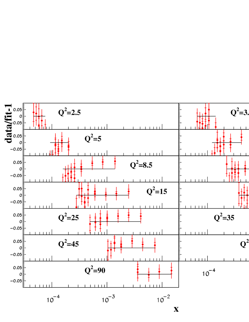
It is instructive to study the pulls of the individual data sets included in the fit. This provides a mean of assessing the quality of the fit in detail and allows for an investigation of specific kinematical regions. In Figs. 4.1–4.3 we display the detailed dependence of the pulls on the momentum transfer and for the HERA NC and CC inclusive DIS cross section data of [18] as well as the low data of [31] with respect to our NNLO fit. We find overall a very good description of the data, even at the edges of the kinematical region of HERA, i.e., at smallest values of and largest values of . The respective values for the fit at NLO and NNLO are given in Tab. 4.2.
| Experiment | NDP | |||
|---|---|---|---|---|
| DIS inclusive | H1&ZEUS [18] | 486 | 537 | 531 |
| H1 [31] | 130 | 137 | 132 | |
| BCDMS [82, 83] | 605 | 705 | 695 | |
| NMC [84] | 490 | 665 | 661 | |
| SLAC-E-49a [77] | 118 | 63 | 63 | |
| SLAC-E-49b [77] | 299 | 357 | 357 | |
| SLAC-E-87 [77] | 218 | 210 | 219 | |
| SLAC-E-89a [78] | 148 | 219 | 215 | |
| SLAC-E-89b [79] | 162 | 133 | 132 | |
| SLAC-E-139 [80] | 17 | 11 | 11 | |
| SLAC-E-140 [81] | 26 | 28 | 29 | |
| Drell-Yan | FNAL-E-605 [90] | 119 | 167 | 167 |
| FNAL-E-866 [91] | 39 | 52 | 55 | |
| DIS di-muon | NuTeV [95] | 89 | 46 | 49 |
| CCFR [95] | 89 | 61 | 62 | |
| Total | 3036 | 3391 | 3378 |
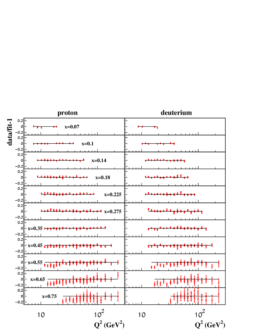
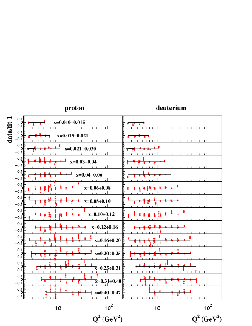
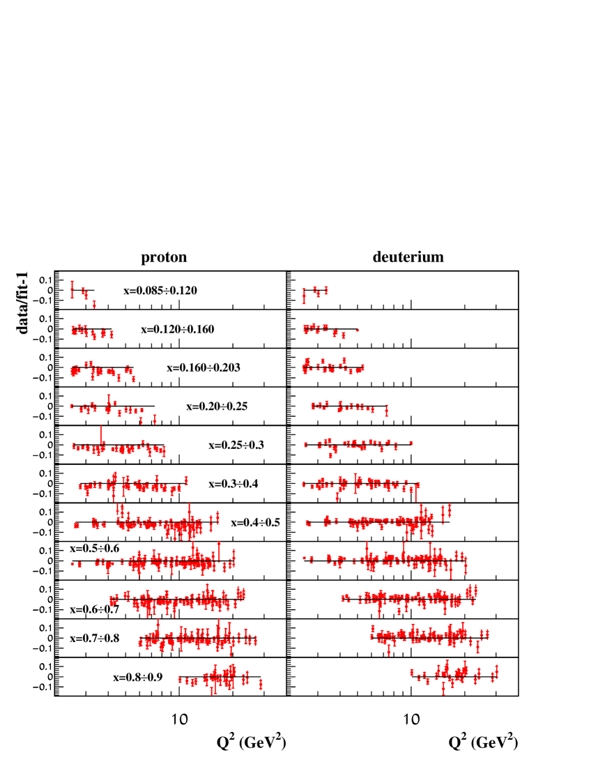
Next, in Figs. 4.4–4.6 we show the respective pulls of the BCDMS [82, 83], NMC [84] and SLAC [78, 77, 81, 80, 79] inclusive DIS cross section data as a function of and binned in the momentum transfer . Again, our fit provides a very good description (see Tab. 4.2 for the values), especially at low thanks the phenomenological ansatz for the structure functions with the higher twist terms of Tab. 4.3.
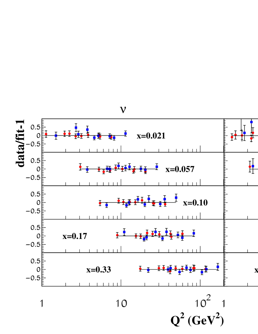
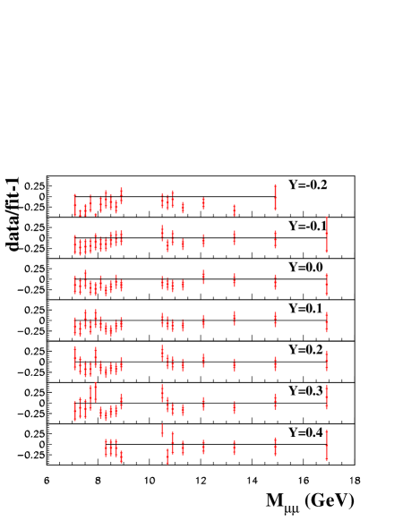
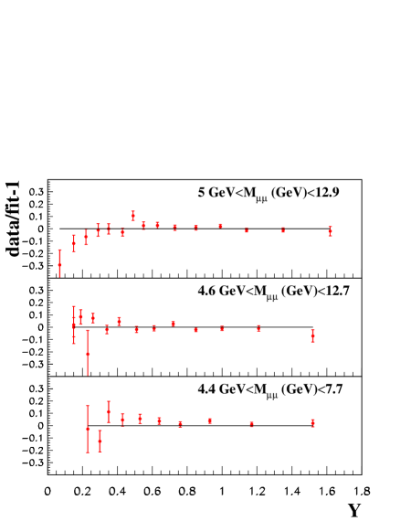
In Fig. 4.8 we plot the data for the (anti-)neutrino induced di-muon production cross section of [95] which constrains the strange PDF. We give both, the pulls for the NuTeV and for the CCFR experiment. Finally, in Fig. 4.8 we display the DY cross section data of [90, 91] which depends on the muon pair rapidity and the invariant mass of the muon pair and which assists in the flavor separation of the PDF fit. It is obvious from Figs. 4.8, 4.8 and Tab. 4.2 that we achieve again a very good description in all cases.
| -0.036 0.012 | -0.034 0.023 | -0.091 0.017 | |
| -0.016 0.008 | 0.006 0.017 | -0.061 0.012 | |
| 0.026 0.007 | -0.0020 0.0094 | 0.0276 0.0081 | |
| 0.053 0.005 | -0.029 0.006 | 0.031 0.006 | |
| 0.0071 0.0026 | 0.0009 0.0041 | 0.0002 0.0015 |

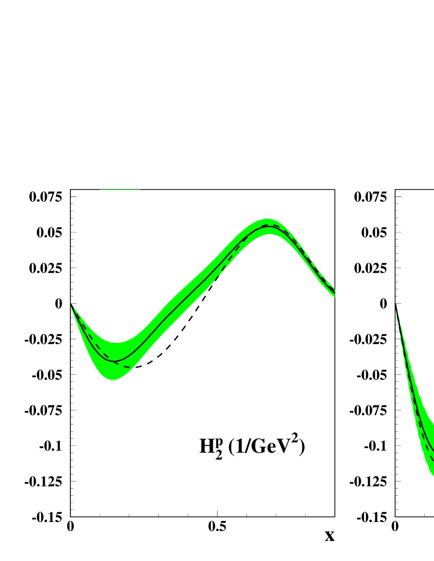
The last missing piece of information on the PDF fit concerns the shape of the higher twist terms for the inclusive DIS structure functions introduced in eq. (2.12). As outlined in Sec. 2.2 we fit three twist-4 coefficients for a complete description of both, proton and nucleon targets. In detail, the proton , the non-singlet and the proton contribute 15 parameters in total and we assume . The respective coefficients are listed in Tab. 4.3 and shown in Fig. 4.9, all in units of , They are in agreement with the earlier results of [59, 60] up to the parameterization of the HT contribution (compare eq. (2.12) with eq. (35) of [60]). The magnitude of the HT terms reduces from the NLO to the NNLO case, see Fig. 4.9, however the change is comparable with the coefficient uncertainties and the NNLO twist-4 coefficients do not still vanish, in line with the results of [60]. The non-singlet twist-4 term in is comparable to zero within uncertainties therefore it was fixed at zero in our analysis as discussed in Sec. 2.2. The non-singlet twist-4 term in is negative at . This is also in line with earlier results [59], again taking into account the difference in the HT parameterizations. The HT terms are mostly important at small hadronic invariant mass . This was confirmed in a comparison of the low- JLAB data [100] with predictions based on the ABKM09 PDFs with account of the twist-4 terms, which were extracted in the analysis of [16] similarly to the present one. However even with the cut of as commonly imposed in global PDF fits the HT terms are numerically important for the region of , which is not affected by this cut.
From Fig. 4.10 it is evident, that calculations, which are based on our NNLO PDFs, but do not include the HT terms, systematically overshoot the SLAC data at due to the HT terms being negative in this region. The value of for the SLAC data at
| (4.11) |
is 699/246 in this case. This is much worse than the value of obtained in our fit for the same subset of data. We have also performed similar comparisons taking the published 3-flavor NNLO MSTW [22] and NLO NN21 [99] PDFs as an input of our fitting code. The NNLO MSTW and NLO NN21 predictions obtained in this way without accounting for the HT terms and with the cut of eq. (4.11) imposed lead to poor a description of the SLAC data, cf. Fig. 4.10. For the case of NN21 PDFs the agreement with the data is particularly bad, with an off-set reaching up to at and a value of . The MSTW value of is also far from ideal in this case, obviously due to the missing HT terms. Also, MSTW does not take into account the target mass corrections. Note, that for the comparison performed without the twist-4 terms the ABM11 value of is worse than ones of MSTW and NN21 since those PDFs are obtained disregarding the HT terms. This also shows that parts of the twist-4 terms obtained in our fit are effectively absorbed into the MSTW and NN21 PDFs.
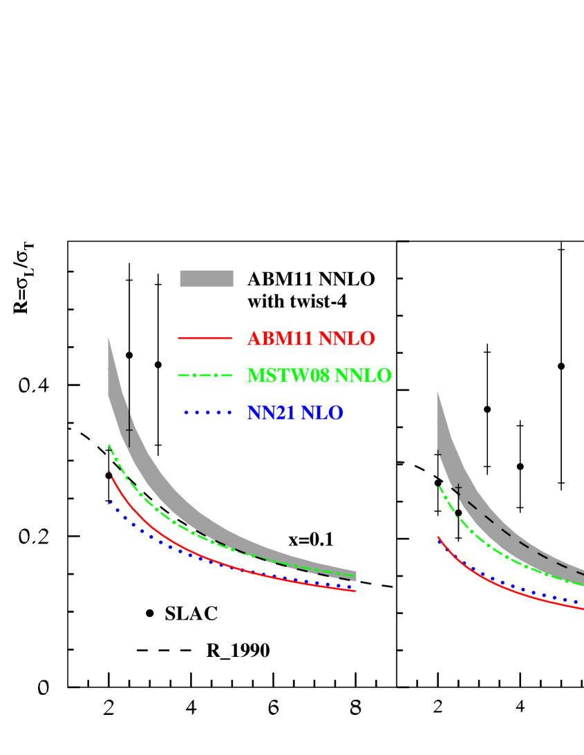
The relative contribution of the higher twist terms to the ratio in eq. (3.2) is particularly important reaching up to one half at moderate [101]. The value of calculated including the NNLO QCD corrections and the twist-4 terms of Tab. 4.3 is in reasonable agreement with the SLAC data on [62] and the parameterization of those data , see cf. Fig. 4.11. The latter is based on the empirical combination of the QCD-like terms with the twist-4 and twist-6 terms, pretending to describe the data down to scales . Due to the twist-6 term, which provides saturation of at small , the shape of is somewhat different from our calculation, while both agree with the data at within the errors. The leading twist NNLO contribution to undershoots the full calculation by a factor of , depending on , cf. Fig. 4.11. The leading-twist NLO calculations based on the 3-flavor NN21 PDFs are in a good agreement with our NNLO leading-twist term and go by factor of lower than the data as well. The leading-twist NNLO calculations for the 3-flavor MSTW PDFs are larger than the NLO NN21 ones and are in better agreement with the data. Note, that this is related to the fact that the data on of [62] are included into the MSTW fit allowing for a better description of the SLAC cross section data as compared to the NN21 case, see Fig. 4.10 and the related discussion above. At the same time this leads to an effective absorption of the twist-4 terms into the fitted PDFs.
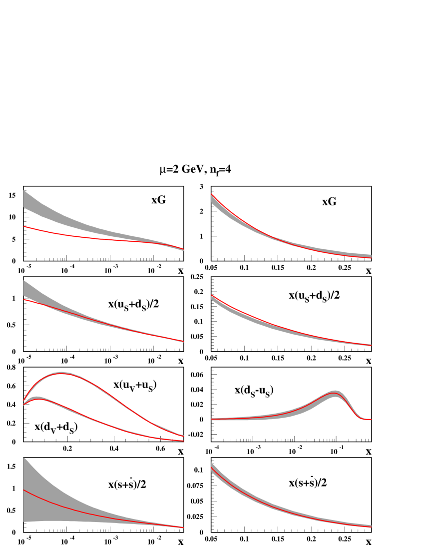

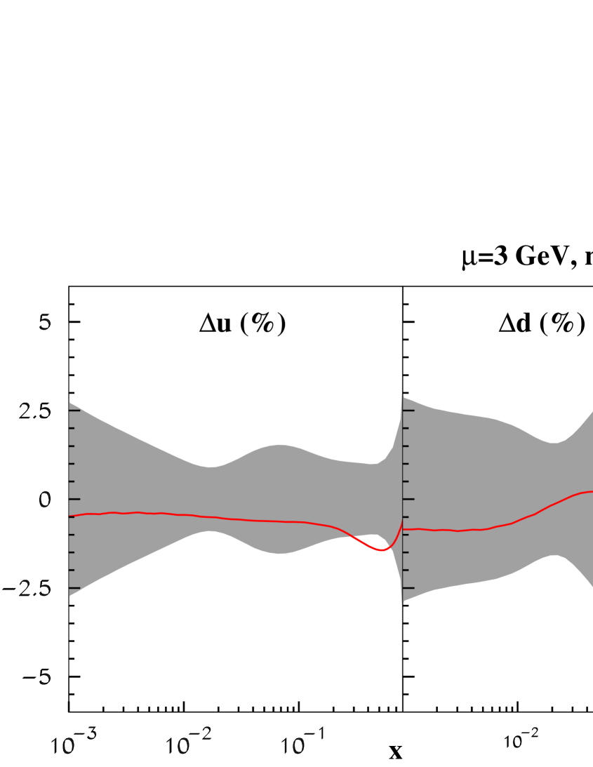
The NNLO ABM11 PDFs obtained in the present analysis are compared in Fig. 4.12 with our earlier ABKM09 PDFs. The biggest change between these two sets is observed for the small- gluon and sea distributions. Firstly, this change happens since the HERA NC inclusive data [18] used in the present analysis lie by several percent higher than the HERA data of [87, 86] used in the ABKM09 analysis, due to improvements in the monitor calibration. Secondly, the small- PDFs are particularly sensitive to the treatment of the heavy-quark electro-production and, therefore, they change due to the NNLO corrections and the running-mass scheme implemented in the present PDF fit. Other ABM11 PDFs are in agreement with the ABKM09 ones within the uncertainties.
The NNLO PDFs obtained by other groups are compared with the NNLO ABM11 PDFs in Fig. 4.13. The agreement between the various PDFs is not ideal, a fact that may be explained by the differences in the data sets used to constrain the PDFs, by the factorization scheme employed, by the treatment of the data error correlation and so on. A detailed clarification of these issues is beyond the scope of the present paper. Therefore we discuss only the most significant differences, e.g., the gluon distributions at small , which are quite different for all PDF sets considered in Fig. 4.13.
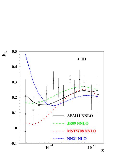
To that end, we compare in Fig. 4.14 the small- data on obtained by the H1 collaboration [31] with the predictions based on these PDFs. The data are quite sensitive to the small- gluon PDFs. Moreover, in order to provide a consistent comparison all predictions are taken in the running-mass 3-flavor scheme with the heavy-quark masses of eq. (4.10) and with the 3-flavor PDFs. The H1 data on are in a good agreement with the NNLO ABM11 predictions. Although these data were not included into the fit of [20] they are also in a good agreement with the NNLO JR09 predictions. The NNLO MSTW and NLO NN21 predictions on the other hand miss the H1 data. Thus, the latter can be used to consolidate the small- behavior of the gluon PDFs provided by different groups. Likewise, the SLAC DIS cross section data of [78, 77, 81, 80, 79] can also be of help in consolidating the results of the different PDF fits. As one can see in Fig. 4.10 the MSTW and NN21 predictions systematically overshoot the SLAC data at . As we discussed above, this happens due to the omission of the higher twist terms. Once the latter are neglected in the fit, the power corrections are partially absorbed in the leading twist PDFs. Therefore, this discrepancy is evidently also related to the difference of those PDFs with the ABM11 ones at moderate , cf. Fig. 4.13. On the other hand, the ABM11 large- gluon distribution goes lower than the NN21 and MSTW ones, because we do not include the Tevatron inclusive jet data into the fit, cf. [102] and Sec. 5.4.
Another striking difference in Fig. 4.13 is related to the strange sea distribution, which is commonly constrained by the data on the di-muon production in the DIS in all PDF fits considered. Nonetheless, for the NN21 and JR09 sets it goes significantly lower at than for the MSTW and ABM11 ones. The difference between the NN21 and ABM11 strange sea distributions appears to be due to eq. (34) of [99] for the di-muon production cross section, which contains an additional factor of as compared, e.g., to eq. (3) of [38] employed in our analysis, cf. also [50]. At small this factor reaches a numerical value of 2 and the strange sea is suppressed correspondingly in the fit to the data. We have convinced ourselves that with this factor taken into account the NN21 PDFs deliver a satisfactory description of the CCFR and NuTeV di-muon data. On the other hand, the discrepancy between the results of JR09 and ABM11 in Fig. 4.13 can directly be traced back to the ansatz of JR09, i.e., the assumption of vanishing strangeness at the low starting scale of in the dynamical valence-like PDF model of JR09. This is different from ours, cf. eq. (4.4). Moreover, JR09 has not used the data on di-muon production in neutrino-nucleon collisions in their fit, see Sec. 3.3.
Finally, the difference in the large- non-strange quark distributions appears partly due to the general normalization of the data, which is often a matter of choice in the PDF fits. In order to quantify impact of the choice of the data normalization on the PDFs (cf. Sec. 3), we have performed a variant of our NNLO fit with the same normalization factor settings as employed in the MSTW fit [22]. The relative difference between the - and -quark distributions obtained in this variant of the fit and our nominal one is displayed in Fig. 4.15. Clearly, the impact of the data normalization choice is most pronounced at large , where the trend is different for the cases of - and -quarks. Therefore the effect is amplified in the ratio which is important for the interpretation of the charged-lepton asymmetry data from hadron colliders, cf. Sec. 5.1. As shown in Fig. 4.15, the relative difference in the ratio reaches up to 5% at .
4.2 Strong coupling constant
| Experiment | |||
|---|---|---|---|
| NLOexp | NLO | NNLO | |
| BCDMS | |||
| NMC | |||
| SLAC | |||
| HERA comb. | |||
| DY | |||
| ABM11 | |||
| Experiment | |||
|---|---|---|---|
| NLOexp | NLO | NNLO∗ | |
| D0 1 jet | |||
| D0 2 jet | |||
| CDF 1 jet (cone) | |||
| CDF 1 jet () | |||
| ABM11 | |||

For a precision determination of the fit of systematically compatible data sets is a necessary prerequisite. Here the individual data sets determine the average in such a way that their individual effect is closely compatible with the central value within the errors. Enhancing the precision from NLO to NNLO, and in some cases to even higher orders, the central values and the values obtained for the individual data sets both stabilize. Moreover, the values of obtained by individual experiments, capable to measure from their data alone, have to be consistently reproduced. One observes a decreasing sequence of differences between the sequential orders, cf. e.g., [60, 110].
In the present analysis based on the measured scattering cross sections and with account of higher twist contributions, c.f. also [27] we obtain from the data sets described in Sec. 3,
| (4.12) | |||||
| (4.13) |
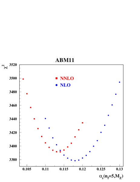
The value at NNLO is shifted by downward if compared to the NLO value. This range of uncertainty is well compatible with the scale uncertainty observed in a variation of the factorization and renormalization scales at NLO of , cf. [111]. The present data allow a measurement of with an accuracy of . Therefore NNLO analyses are mandatory, since the NLO results exhibit much too large theory errors. The response to the fitted -dependence is measured using the functional of eq. (A.1). In Fig. 4.16 the dependence of of is illustrated at NLO and NNLO.
In Tab. 4.4 we compare the values for obtained for the individual data sets at NLO and NNLO in the present fit and with results obtained by some of the experiments. Here the -value for BCDMS was re-evaluated using the value of MeV and [83]. These values correspond to a NLO fit with in the -scheme. We evolved this value back to the charm threshold keeping and determined then evolving forward passing the bottom threshold. In [59] higher twist contributions and were fitted together for the BCDMS and data resulting in the somewhat larger value MeV and the NLO value , which was also obtained [60, 110]. Both values are compatible within errors.
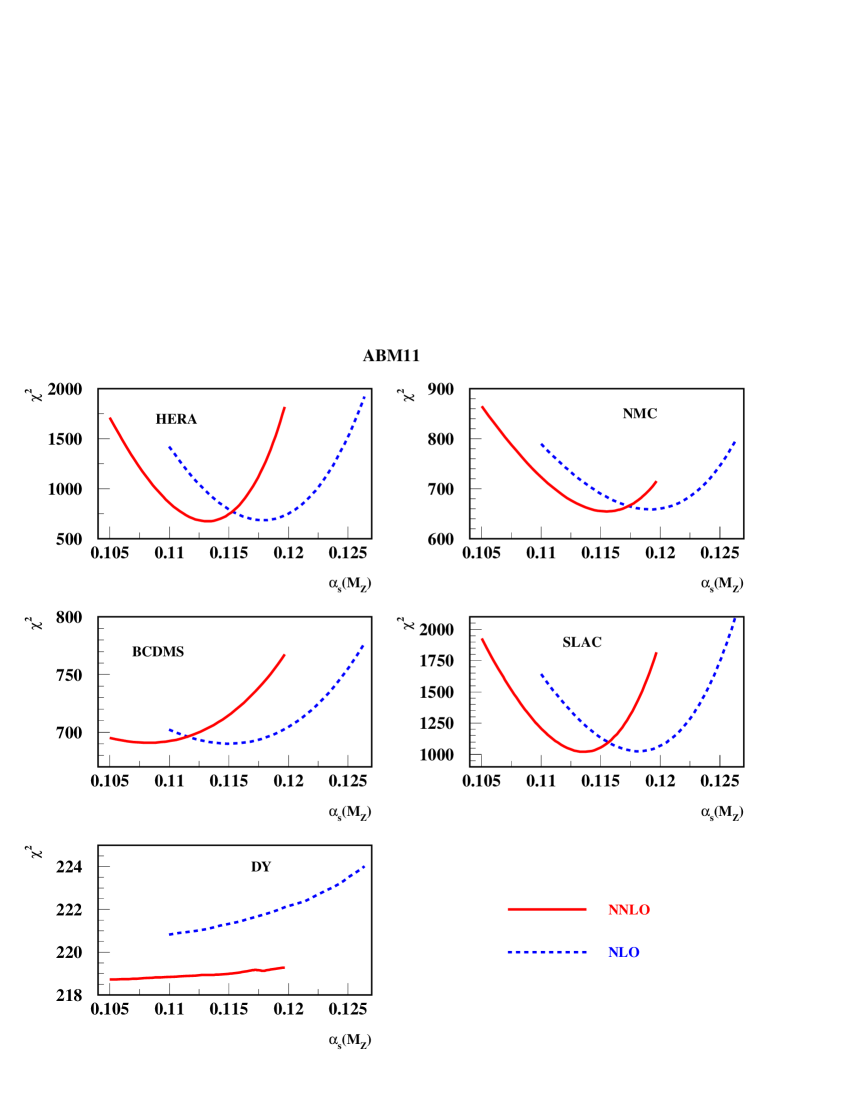
In Fig. 4.17 we plot the -profile using eq. (A.1) at NLO and NNLO. To that end, we compare the fit result with the -behavior of the individual data set, fixing all other parameters. The minimum and variation () then determine the values given in Tab. 4.4, see also Fig. 4.17. For BCDMS and NMC we find complete consistency to the values given by the experiments and the present analysis. The downward shift which is consistently observed when going from NLO to NNLO amounts to values between 0.0030 and 0.0055, with a lower sensitivity for the DY data, which yield rather low values with large errors. The fitted central values are well covered by the individual data sets. Fig. 4.17 shows the response with respect to of the individual data sets fixing the non-perturbative shape parameters in the global fit. One may refit these parameters in changing , cf. Fig. 4.18. However, here the change in the other PDF parameters remains undocumented, in particular if the corresponding covariance matrices are not publicly available, as is the case for some of the global fits. We have performed this analysis only to compare to the MSTW and NNPDF analyses below but still prefer the results of Fig. 4.17. Both results are given in Tab. 4.9 for comparison. Comparing Figs. 4.17 and 4.18 one finds that the shape parameters in case of the BCDMS and HERA data remain widely stable and larger shifts are introduced for the NMC and SLAC data. The stability of the results, on the other hand, allows to conclude that fully compatible sets of precision data were used.
We have also performed NLO fits, including the Tevatron jet data [105, 106, 107, 108]. Furthermore, we have formally extended the analysis fitting the DIS and DY data at NNLO while treating the Tevatron jet data at NLO and supplementing threshold corrections based on soft gluon resummation [109] for the single jet inclusive data. This latter approximation we denoted by NNLO∗, cf. [102]. A NLO measurement of was also performed by CDF [112], with larger errors than in [104], . At NLO the different sets of Tevatron jet data do not modify the value obtained in our standard analysis. A consistent NNLO is not yet possible since the corresponding scattering cross sections still have to be calculated. Again a systematic downward shift of is obtained upon going from NLO to NNLO∗. The corresponding central values are 1 compatible with our NNLO central value in eq. (4.13). We would like to mention that already our former ABKM09 results [16] give a very good description of the CMS jet data [113] and also the Tevatron 3-jet data [114]. We note that in a recent NLO analysis of the 5-jet cross section at LEP a value of was obtained [115].


The higher twist terms play an important role in the determination of from the DIS data [59]. In our analysis they contribute up to 10% of the cross section at the low margin of and given by eq. (3.3). As a result, the value of is strongly correlated with the twist-4 coefficients, which are extracted from the fit simultaneously with , cf. Fig. 4.19. The correlation is more pronounced for at large and for at small . The latter affects the determination of even in the case of a more stringent cut on since the low- part of the data is not sensitive to this cut. For the variant of our NNLO fit with the cut of eq. (4.11) imposed and the higher twist terms set to zero, we obtain the value of , much bigger than our nominal result of eq. (4.13). For comparison, the same fit with the higher twist terms fixed at the values of Tab. 4.3 gives comparable with eq. (4.13). Note that in both cases the error in is smaller than one of eq. (4.13) despite the reduced data set used in the fit. This says, that the uncertainty in is essentially controlled by the higher twist term variation. To get rid of the impact of the higher twist terms on an even more stringent cut on is necessary, in addition to the cut on . With the NNLO variant of our fit and using
| (4.14) |
the value of is obtained, if the higher twist terms are set to zero and , if the higher twist terms are fixed at the values of Tab. 4.3. From this comparisons we conclude that is pushed to larger values due to the neglect of the higher twist terms in the case of a cut as in eq. (4.11), which is commonly imposed in the global PDF fits. Likewise, it is less sensitive to the details of the fit ansatz. As we have found earlier [27], the value of extracted from our fit is quite sensitive to the treatment of the NMC data [88]. Normally, we use the NMC data on the cross section in the fit, cf. Sec. 3.1. If, however, we employ instead the NMC data on extracted by the NMC collaboration with their own assumptions about the value of , the value of increases by for the case of our earlier ABKM09 NNLO fit [27]. In comparison, for the variant of the ABKM09 with the cut of eq. (4.11) imposed and the high-twist terms set to zero, the value of is shifted by only. This is in agreement with the size of the variation obtained in the variant of the MSTW08 fit with an improved treatment of the NMC data [28]. Note, however, that the details of the DIS data treatment employed in the improved analysis of [28], are still different from ours. In places, this has an impact on the value. E.g., if we combine the errors in the NMC and HERA data in quadrature, as it is done in [28, 22], the NNLO ABKM09 value of is shifted upwards by and its sensitivity to the NMC data treatment is reduced to . This effect may in particular explain the relatively big value of observed in [28] with the cuts similar to ones of eq. (4.14).
The impact of the NMC data treatment on the fit has also been studied for NN21 in [30], where little effect on the PDFs has been found. However the value of obtained in that analysis is still much lower than the one obtained in our fit and closer to the value of used by NMC to extract the value of from the cross section (compare Fig. 2 in [30] and Fig. 1 in [27]). Note in this context that the value of obtained in [30] for the NMC data is much bigger than in our case, cf.Tab. 4.2. Furthermore, in the NN21 study the value of is fixed. Therefore, its correlation with the PDFs is not considered. Finally, the expressions for cross sections used in the NN21 analysis do not include the power corrections in , which are numerically important at small (compare eqs. (2), (3) in [30] with eq. (1) in [88], and eqs. (3.1), (3.2) of the present article). These differences make a detailed comparison of the results of [27] and [30] difficult.
The value of obtained in our fit is substantially constrained by the BCDMS data of [82, 83], which almost entirely survive after the cut of eq. (3.3). Meanwhile the authors of [116] suggested to cut in addition the most inaccurate BCDMS data with low inelasticity . The value of reported in [116] with such cut is by larger than the one obtained from the analysis of the whole set of the BCDMS data at NNLO. The pulls of the low- data rejected in the analysis of [116] with respect to our NNLO fit are given in Fig. 4.20. The fit is in reasonable agreement with data within the errors. Furthermore, rejecting these data points from the NNLO fit, we obtain a value of , which is somewhat bigger than the one in eq. (4.13). The statistical significance of the shift, however, is marginal. The discrepant findings of [116] concerning the impact of the low- BCDMS data may appear due to the fact that the systematic uncertainties in the data are not taken into account in [116]. In our case the systematic errors are included into the value of , cf. Sec. A. Therefore the low- data points with an enhanced systematic uncertainty have reduced weight and do not affect the fit.
| Experiment | ||||
|---|---|---|---|---|
| NLOexp | NLO | NNLO | N3LO∗ | |
| BCDMS | ||||
| NMC | ||||
| SLAC | ||||
| BBG | ||||
| BB | ||||
We turn now to comparisons with other NNLO analyses which will be performed studying the contribution of different data sets to . We first compare to the flavor non-singlet analyses [60, 110]. In [110] the valence analysis is performed by accounting for the remnant sea-quark and gluon contributions to in the region through the PDFs taken from [16]. The results are summarized in Tab. 4.6. The values of at NLO turn out to be lower than those obtained in singlet analyses, cf. Tabs. 4.4 and 4.10. However they are consistent within the scale variation errors. At NNLO both analyses lead to the same values. Also note the anti-correlation of the size of higher twist contributions in the large- region with the inclusion of higher orders at leading twist, cf. [67, 60, 61, 110]. The next order, denoted by N3LO∗, yields information on the remaining theoretical uncertainty. At N3LO∗, the non-singlet three-loop Wilson coefficients are used [9, 10] and the four-loop non-singlet anomalous dimension is estimated with a Padé-approximation and accounting for a 100 % error. In fact the latter extrapolation agrees within with the second moment of the non-singlet four-loop anomalous dimension [120, 121]. For the three experiments, which give the bulk information on , the shift due to the N3LO∗ contributions amount to and globally to 0.0007. At NNLO, the values of the individual data sets vary by 0.0032, consistent within the 1 errors.
Next, in Tab. 4.7, we compare with the fit results of NN21 [122, 123] for individual data sets for DIS and other hadronic hard scattering data. The labels for those data sets in Tab. 4.7 follow the original notation of NN21 in [122, 123] (and, likewise in Tab. 4.8 for MSTW [159]). The references corresponding to the data sets are given additionally. At NLO the values range from 0.1135 (E866, DY) to 0.1252 (NuTeV), with a corresponding range at NNLO of 0.1111 (D0 jet) to 0.1225 (CDF jet). The value of for the BCDMS data at NLO differs significantly from that given by the experiment [83]. Comparing the change of the values between the NLO and NNLO analyses one finds downward shifts between 0.0075 (NuTeV) and 0.003 (CDF R2KT) and upward shifts between (CDF Zrap) and (ZEUS H2), see Tab. 4.7. The values for obtained for the SLAC data are found to be larger than 0.124 both at NLO and NNLO, cf. Fig. 2 in [123]. The values for the scans in at NNLO turn out to be worse than in NLO in the global analysis for the data sets of NMC, BCDMS, HERA I, CHORUS, ZEUS F2C, DY E866, CDF Zrap, and D0 Zrap, again see Fig. 2 in [123]. Comparing the DIS only fit to the global analysis it is found that the values improve significantly, except for NMCp, and to a lesser extent for SLAC at higher values of , cf. Fig. 5 in [123].
| Experiment | |||
|---|---|---|---|
| NLOexp | NLO | NNLO | |
| BCDMS [82, 83] | |||
| NMCp [84] | |||
| NMCpd [124] | |||
| SLAC [119] | |||
| HERA I [18] | |||
| ZEUS H2 [125, 126] | |||
| ZEUS F2C [127, 128, 129, 130] | |||
| NuTeV [95, 96] | |||
| E605 [90] | |||
| E866 [92, 131, 91] | |||
| CDF Wasy [132] | |||
| CDF Zrap [133] | |||
| D0 Zrap [134] | |||
| CDF R2KT [105] | |||
| D0 R2CON [107] | |||
| NN21 | |||
| Experiment | |||
|---|---|---|---|
| NLOexp | NLO | NNLO | |
| BCDMS [82] | |||
| BCDMS [83] | |||
| NMC [84] | |||
| NMC [84] | |||
| NMC [124] | |||
| E665 [135] | |||
| E665 [135] | |||
| SLAC [62, 89] | |||
| SLAC [62, 89] | |||
| NMC,BCDMS,SLAC, [82, 84, 119] | |||
| E886/NuSea , DY [131] | |||
| E886/NuSea , DY [91] | |||
| NuTeV [136] | |||
| CHORUS [137] | |||
| NuTeV [136] | |||
| CHORUS [137] | |||
| CCFR [95, 96] | |||
| NuTeV [95, 96] | |||
| H1 97-00, [138, 139, 86, 140] | |||
| ZEUS 95-00, [141, 87, 142, 143] | |||
| H1 99-00, [139] | |||
| ZEUS 99-00, [144] | |||
| H1/ZEUS [127, 128, 145, 146, 147, 148] | |||
| H1 99-00 incl. jets [149, 150] | |||
| ZEUS 96-00 incl. jets [151, 152, 153] | |||
| D0 II incl. jets [107] | |||
| CDF II incl. jets [105] | |||
| D0 II asym. [154] | |||
| CDF II asym. [155] | |||
| D0 II rap. [134] | |||
| CDF II rap. [156] | |||
| MSTW | |||
| Data Set | ABM11 | BBG | NN21 | MSTW |
|---|---|---|---|---|
| BCDMS | ||||
| () | ||||
| NMC | ||||
| () | ||||
| SLAC | ||||
| HERA | ||||
| DY | ( | |||
| BBG | valence analysis, NNLO [60] | |
| BB | valence analysis, NNLO [110] | |
| GRS | valence analysis, NNLO [161] | |
| ABKM | HQ: FFNS [16] | |
| ABKM | HQ: BSMN-approach [16] | |
| JR | dynamical approach [20] | |
| JR | standard fit [20] | |
| ABM11 | ||
| MSTW | [159] | |
| NN21 | [123] | |
| CT10 | [162] | |
| Gehrmann et al. | thrust [163] | |
| Abbate et al. | thrust [164] | |
| 3 jet rate | Dissertori et al. 2009 [165] | |
| Z-decay | BCK 2008/12 (N3LO) [166, 167] | |
| decay | BCK 2008 [166] | |
| decay | Pich 2011 [168] | |
| decay | Boito et al. 2011 [169] | |
| lattice | PACS-CS 2009 (2+1 fl.) [170] | |
| lattice | HPQCD 2010 [171] | |
| lattice | ETM 2012 (2+1+1 fl.) [172] | |
| BBG | valence analysis, N3LO [60] | |
| BB | valence analysis, N3LO [110] | |
| world average | [173] (2009) | |
| [168] (2011) |
In Tab. 4.8 the values determined by MSTW at NLO and NNLO [159] are compared for individual data sets in the fit. Here, the 1 errors, as defined by MSTW, are read off the corresponding plots in [160]. This definition of ‘1’ is obtained for values of much larger than one. Moreover, these values do even strongly vary between the different measurements used, which is unlike the case for the ABM and NN21 analyses. This procedure leads to an enlargement of errors, which, e.g., in the case of BCDMS translates into a NNLO value rather than the experimental one of . The latter accuracy is reflected in other analyses, however, cf. (BB), (NN21), and (ABM11). Similar effects are present for various other data sets, as can be seen comparing the values given in Tabs. 4.4–4.8. In this way, almost all individual -errors, even at NNLO, are larger than the typical theory uncertainty of about at NLO. We stress that the present analysis (ABM11) correctly accounts for the experimental systematic errors of all data sets used, cf. Tabs. 4.4 and 4.5, and that an enlargement of errors has not been necessary. In view of this fact, it is somewhat surprising that the final error in the MSTW analysis, i.e. (MSTW), fully agrees with those obtained by BB, ABM11, and NN21, cf. Tab. 4.9. Unlike the case of NN21, the values of MSTW become generally lower at NNLO if compared to NLO, with the exception of the D0 run II -boson rapidity data set, where the NNLO value is slightly higher.
It is also interesting to compare the values obtained in the NN21 [122, 123], MSTW [159] and ABM11 analyses with respect to the individual data sets used in those fits. At NLO NN21 obtains lower values for D0 R2CON than MSTW and ABM and a significantly higher value for D0 ZRAP than MSTW, see Tabs. 4.7 and 4.8. At NNLO, the individual value for the data set CDF Zrap moves upward with respect to the NLO value with a significantly larger error, while for MSTW the value remains the same as at NLO. The values of ABM11 given in Tab. 4.5 for Tevatron jet data are rather close to those of MSTW, both at NLO an NNLO∗. For the NuTeV data the NLO and NNLO values show a bigger difference for NN21 than for MSTW, while the NNLO values are rather similar.
In Tab. 4.9 we compare the values of the ABM11, BBG, NN21 and MSTW analyses for those data sets which are commonly used at NNLO. An NLO comparison would still be subject to a scale error of , which is usually too large to differentiate between the various fit results. For ABM11 we present the values extracted from Figs. 4.17 and 4.18. For the BCDMS data ABM11, BBG and MSTW obtain lower values, while NN21 differs, e.g., by (or ) from MSTW and (or ) from ABM11. For the NMC data ABM, BBG, and NN21 do agree very well, while the value of MSTW shows an upward shift of compared to NN21. The size of both these shifts is of the order of NLO scale uncertainty and should not be present at NNLO. For the SLAC data the values by ABM11, BBG and MSTW are consistent within errors. On the other hand, MSTW reports a much larger value for the SLAC data than obtained by ABM11 and BBG. NN21 obtains partial values both at NLO and NNLO both in their global and DIS only analyses. This is in contrast to the present results, to BB, and to MSTW for the data. In the non-singlet BBG analysis the influence of the HERA data is strongly reduced, since most of these data are located within the quark-sea region. The fit results of NN21 and MSTW lead to values of while those of ABM11 yield a much lower value of 0.1139 (0.1126). Note that the MSTW analysis does not yet include the HERA run I combined data set [18]. The results for the DY data are consistent between ABM11 and MSTW, although the sensitivity of these data to is comparably small. In summary, despite the fact that NN21 and MSTW obtain nearly the same global fit values for , the above discussion shows that quite a series of individual pulls are different. Both ABM11 and MSTW do not confirm the relatively large values for the data sets of BCDMS and CDF R2KT and also the rise, at NNLO, of the NN21 value for CDF Zrap calls for further clarification, cf. Tab. 4.7.
Summarizing the comparison of the present results on with the analyses [60, 110, 122, 123, 159, 160] we observe a good agreement with [60, 110] and find differences in a series of data sets for [122, 123, 159, 160] both at NLO and NNLO, with partly different deviations in case of [122, 123] and [159, 160]. NN21 does not agree with the BCDMS result. We find lower values of both for the HERA and the SLAC data. We do not confirm part of the values found in [122, 123, 159, 160] for the jet data. We would like to mention once more that in our analysis no rescaling of errors is performed, which varies for different data sets in the analysis [159, 160], but we have accounted for the systematic errors given by the experiments directly. The procedure of[159, 160] naturally leads to re-weighting of the impact of different data sets on the value of .
Finally we would like to summarize the results of different determinations of at NNLO and N3LO (or N3LO∗) in Tab. 4.10. Some part of these results has been reported in [168]. Flavor non-singlet analyses of the DIS world data were performed in [60, 161, 110], with an accuracy of at NNLO. The difference between the value at N3LO∗ and NNLO amounts to , which provides an estimate for the size of a remaining uncertainty. The ABKM09 analysis [16] is a combined flavor singlet/non-singlet fit of the DIS world data, DY and di-muon data. Here a remaining difference of due to the treatment of the heavy-flavor corrections was observed. These uncertainties signal the typical theory errors remaining at the present level of description. The JR09 analysis obtained very similar results in combined flavor singlet/non-singlet fits [20] with a slightly larger value in the standard fit compared to the dynamical approach. The present analysis obtains the same values as those found in [60, 110, 16, 161, 20] before, while a slightly larger value was reported in ABM10 [17] based on incorporating the combined HERA run I data [18]. However, the improved treatment of the heavy-quark contributions finally led to the present value . The inclusion of Tevatron jet data, cf. [102], although only a NNLO∗ analysis, alters this values at most to and the effect of the complete, yet unknown NNLO corrections, remain to be seen. Low values of have not only been reported in analyses which are predominantly based on DIS data, but also from those of thrust in -annihilation in [164], cf. also [163].
Larger central values of at NNLO (and similar in size) are reported by MSTW [159] and NN21 [123]. These fits include a much broader set of hadronic scattering data in the analysis and above we have pointed out various differences between these analyses, see Tabs. 4.7 and 4.8. These differences manifest themselves in various cases in rather different pulls for the value of . Note also that the 1 confidence level is very differently defined in the MSTW analysis compared to ABM11, NN21 and JR09. The (preliminary) central value of reported by CT10 [162] is similar to MSTW and NN21 at NNLO, although accompanied by a rather large uncertainty of , which makes the CT10 result compatible with the lower values obtained in [60, 110, 16, 161, 20]. We have also discussed the reasons for the difference between the central values of in the NLO and NNLO analyses [60, 110, 16, 161, 20] and [159, 123] and further comparisons may be performed. An earlier claim that this is caused by the Tevatron jet data is not confirmed, cf. [17]. Larger central values for than in [60, 110, 16, 161, 20] are obtained for the 3-jet rate in annihilation [165] at NNLO and for the -decay width at N3LO [166], see Tab. 4.10. The current values at NNLO extracted from -decays vary between 0.1212 and 0.1169 [166, 168, 169]. One lattice measurement [171] yields the same value as the current world average [168, 173]. Other recent lattice results are compatible with this value and more lattice studies are still underway aiming at improved systematics [174].
4.3 Heavy-quark masses

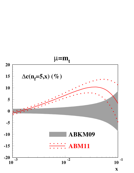

The precise value of the heavy-quark masses is an important parameter in the description of DIS charm-quark production. In our fit we use the heavy-quark masses in the -scheme and their implementation for heavy-quark DIS discussed in [16] which allows us to relate the values for and directly to PDG results [98], as done in eq. (4.10).
The current DIS data displays great sensitivity to the charm mass as we have demonstrated previously [32, 176]. Therefore, based on the pseudo-data input from eq. (4.10) we have released the uncertainty of the quark masses to obtain the following results
| (4.15) |
which shows that the error on from the inclusive DIS data used in the fit is comparable to the one quoted by the PDG [98] (although not comparable to the single most precise measurement listed therein). Interestingly, we observe in the covariance matrix in Tabs. A.1–A.3 correlations of with and some parameters of the gluon and the strange PDFs. The precision of DIS data to the value of has previously also been exploited for the first direct determination of the running mass for charm quarks from hadronic processes with space-like kinematics as a variant of ABKM09 yielding values consistent with but systematically somewhat lower than the PDG world average [32, 176].
It is interesting to compare the results of the fit to the most recent HERA data from the H1 collaboration [175] for the charm structure function in heavy-quark DIS extracted with the use of the HVQDIS code [177]. This is done in Fig. 4.21 for our 3-flavor running-mass NNLO predictions with of eq. (4.15) using the approximate NNLO QCD predictions of [39, 40, 41]. The data are not used in our fit, however the agreement is quite good, as well as for the predictions based on the NNLO 3-flavor PDFs of JR09 [20] and MSTW [22]. The predictions using the NLO 3-flavor NN21 PDFs of [99] undershoot the data. The differences may be related to the peculiarities of the so-called general mass VFNS modeling employed in those fits [22, 24, 99]. Also wrong analyses of the combined H1 and ZEUS data on exist [178].
Finally, we want to mention that the issue of heavy-quark masses also has consequences for heavy-quark PDFs, because the uncertainty on heavy-quark PDFs is directly related to the accuracy of the numerical values for the quark masses or . The latter appear parametrically in the OMEs used to generate charm- and bottom-PDFs in schemes with or flavors. With the results of eq. (4.15) and the use of the -scheme this uncertainty in the charm and bottom PDFs can be significantly reduced.
In Fig. 4.22 we display the PDFs generated in this way. We obtain a charm-PDF with comparable uncertainties to the one of [16] (which then has used the pole mass definition for ), while the resulting uncertainty of the bottom-PDF is greatly reduced, see also [176]. This improvement has a significant impact on LHC phenomenology, as it will, e.g., allow for precise predictions for the production of single-top-quarks and other processes sensitive to bottom-PDFs.
4.4 Moments of the PDFs
| ABM11 | ||||
|---|---|---|---|---|
| ABKM09 [16] | ||||
| HERAPDF1.5 [18, 19] | ||||
| JR09 [20, 21] | ||||
| MSTW [22] | ||||
| NN21 [23] | ||||
| BBG [60] | ||||
| BBG [N3LO] [60] |
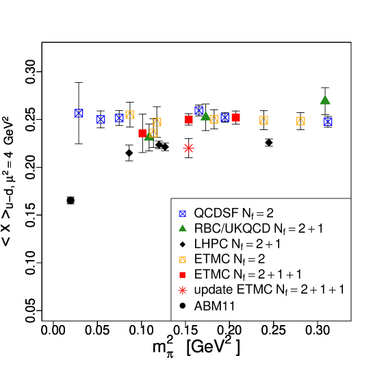
In Tab. 4.11 we summarize different values of the second moment of the valence quark densities obtained in NNLO analyses at the scale . It is evident, that these moments are rather stable quantities for all PDF sets considered as they are mostly influenced by the data normalization. They are closely related to the moments which are being measured in lattice simulations. Of central importance is the quantity
| (4.16) |
where with .
In Fig. 4.23 the result for eq. (4.16) obtained in the present analysis is compared with recent lattice computations using varying numbers of flavors as a function of the pion mass employed on the lattice. In detail, these are QCDSF () [179], RBC/UKQCD () [180], LHPC () [181], ETMC () [182] and ETMC () [183, 184]. It is apparent from Fig. 4.23 that there are substantial differences, even for low pion masses, between those lattice measurements and the experimental determinations of Tab. 4.11. For very recent progress see [185].
5 Benchmarks for cross sections
In this section we quantify the impact of the new PDF set on predictions for benchmark cross sections at the Tevatron and the LHC. To that end, we confine ourselves to (mostly) inclusive cross sections which are known to NNLO in QCD either completely or in very good approximation, see [26] for previous work along these lines. NNLO accuracy is actually the first instance, where meaningful statements about the residual theoretical uncertainty are possible, since at NLO the latter which is conventionally determined from a variation of the renormalization and factorization scale is generally still too large, given the precision of present collider data.
In detail, we consider the following set of inclusive observables: hadronic - and -boson production [11, 12], the cross section for Higgs boson production in the dominant channels, ggF [12, 186, 187, 188], vector-boson fusion (VBF) with VBFNNLO [189, 190], and in Higgs-strahlung [191]. The cross section for top-quark pair production is approximately NNLO (based on threshold resummation, see e.g., [192]) and is computed with HATHOR (version 1.2) [193]. We also consider the lepton () charge asymmetry in hadronic -boson production as a function of the rapidity [13, 14, 15, 194]. Throughout the entire section we focus on the QCD corrections only. That is to say, we neglect all electroweak radiative effects at NLO, which often amount to corrections of at the LHC and, therefore, need to be considered in precision predictions.
The PDF uncertainties quoted here are calculated by summing over the sets provided by the various groups, where is the number of parameters used in the fit. Typically, we quote the symmetric error according to
| (5.1) |
where is obtained by using the -th PDF , which parametrizes the -variation of the -th fit parameter after diagonalization of the correlation matrix. In some cases, e.g., for MSTW [22], asymmetric PDF errors are provided, in which case the variation in the -th fit parameter is given by a pair of PDFs . The resulting asymmetric PDF error is then computed according to
| (5.2) | |||||
| (5.3) |
For MSTW, we are using the set with 68% confidence level error estimates throughout.
In a Monte Carlo approach like the one advocated by NN21 [23], the PDF uncertainty can be determined as the quadratic deviation from the central fit as in Eq. (5.1), but with an additional factor . For reasons of efficiency and run-times, we are using the NN21 PDF with 100 sets in our comparisons only, see also the discussion in Sec. 5.5.
5.1 - and -boson production
We start by presenting results for - and -boson production at the LHC at TeV. For the electroweak parameters, we follow [26] and choose the scheme based on the set . According to [98], we have , GeV, GeV and the corresponding widths GeV and GeV. The weak mixing angle is then a dependent quantity, with
| (5.4) |
and . Finally, the Cabibbo angle yields the value .
At NNLO the theoretical uncertainty due to scale variation is small compared to the PDF error, see Tabs. 5.1 and 5.2. The change in the predictions between ABKM09 and ABM11 is small. NN21 and MSTW typically predict smaller cross sections with differences at the level of 12, while the numbers of JR09 are significantly smaller, see also the detailed discussion in [26]. Most importantly, there is the choice to consider in particular the -boson cross section in alternative schemes with or flavors, since contributions of the initial bottom PDFs being proportional to the CKM matrix element are kinematically suppressed.
| ABM11 | ABKM09 [16] | JR09 [20, 21] | MSTW [22] | NN21 [23] | |
|---|---|---|---|---|---|
Comparing the results in Tabs. 5.1 and 5.2 for the PDF sets with and we observe that the numbers for the scheme are always larger, the differences being less than 1 in the PDF uncertainty, though. These differences, which become successively smaller at higher orders, i.e. as we go from NLO to NNLO accuracy, originate from changes in the light flavor and the gluon PDFs when the bottom PDF is generated perturbatively, recall Sec. 4.3. In summary, the differences between the results in Tabs. 5.1 and 5.2 for a given PDF set constitute an intrinsic uncertainty of the perturbative prediction. Comparisons of heavy-flavor PDFs including mass effects have also been studied in [195].
Next, we address the charged-lepton asymmetry data [196, 197] as obtained by the ATLAS and CMS experiments and compare it to the NNLO predictions based on the ABM11 PDFs in Fig. 5.1. All differential distributions for - and -boson production are computed with the fully exclusive NNLO program DYNNLO [15, 194], which allows to take into account the kinematical cuts imposed in the experiments (cf. Fig. 5.1), see also [198] for an alternative code.
The overall agreement with both experiments is sufficiently good, however at values of for the lepton pseudo-rapidity the data show a different trend with respect to the predictions. Preliminary data on the charge-lepton asymmetry at large rapidities obtained by the LHCb collaboration [199] are also in good agreement with the ABKM09 predictions. To check the impact of the LHC charged-lepton asymmetry data on our fit we have performed a variant of the ABM11 analysis which consists of adding the data of [196, 197]. We have found, however, that the change in the PDF central values and their errors is only marginal in view of still big uncertainties in the data.


5.2 Higgs boson production
Let us now discuss the cross sections for the Standard Model Higgs boson production, where all dominant channels are known to NNLO in QCD.
We start with ggF in Tabs. 5.3–5.5, where the cross section is driven by the gluon luminosity and the value of from the effective vertex. The NNLO QCD corrections obtained in [12, 186, 187, 188] still lead to a sizable increase in the cross section at nominal values of the scale, i.e. . Further stabilization is achieved beyond NNLO on the basis of soft gluon resummation, see e.g., [200].
We observe in Tabs. 5.3–5.5 that the ABM11 predictions are rather stable with small changes only due to the gluon PDF discussed in Sec. 4. The values of MSTW are typically larger than those of ABM11 and of ABKM09, roughly by depending on the Higgs mass and the LHC collision energy, which has direct consequences for the current Higgs searches at the LHC. E.g., at MSTW predicts an 8% larger cross section of which 6.5% are due to the difference in . In terms of PDF uncertainties, this discrepancy is significant at the level of 34. The reasons for the different gluon luminosities in the relevant -range and the value of have been illustrated in Sec. 4. The great sensitivity of the ggF rate to constraints from higher orders in QCD in the treatment of fixed-target DIS data has already been discussed extensively in [27].
| ABM11 | ABKM09 [16] | JR09 [20, 21] | MSTW [22] | NN21 [23] | |
|---|---|---|---|---|---|
| 100 | |||||
| 110 | |||||
| 115 | |||||
| 120 | |||||
| 125 | |||||
| 130 | |||||
| 140 | |||||
| 150 | |||||
| 160 | |||||
| 180 | |||||
| 200 | |||||
| 220 | |||||
| 260 | |||||
| 300 |
| ABM11 | ABKM09 [16] | JR09 [20, 21] | MSTW [22] | NN21 [23] | |
|---|---|---|---|---|---|
| 100 | |||||
| 110 | |||||
| 115 | |||||
| 120 | |||||
| 125 | |||||
| 130 | |||||
| 140 | |||||
| 150 | |||||
| 160 | |||||
| 180 | |||||
| 200 | |||||
| 220 | |||||
| 260 | |||||
| 300 |
| ABM11 | ABKM09 [16] | JR09 [20, 21] | MSTW [22] | NN21 [23] | |
|---|---|---|---|---|---|
| 100 | |||||
| 110 | |||||
| 115 | |||||
| 120 | |||||
| 125 | |||||
| 130 | |||||
| 140 | |||||
| 150 | |||||
| 160 | |||||
| 180 | |||||
| 200 | |||||
| 220 | |||||
| 260 | |||||
| 300 |
| ABM11 | ABKM09 [16] | JR09 [20, 21] | MSTW [22] | NN21 [23] | |
|---|---|---|---|---|---|
| 100 | |||||
| 110 | |||||
| 115 | |||||
| 120 | |||||
| 125 | |||||
| 130 | |||||
| 140 | |||||
| 150 | |||||
| 160 | |||||
| 180 | |||||
| 200 | |||||
| 220 | |||||
| 260 | |||||
| 300 |
Next in size comes the VBF channel. All numbers in Tab. 5.6 are computed with the VBFNNLO program [189, 190] in the structure function approach, which describes VBF as a double DIS process, where two (virtual) vector-bosons (independently) emitted from the hadronic initial states fuse into a Higgs boson. Although the structure function approach to VBF is not truly exact at NNLO it includes the bulk of the radiative corrections so that the remaining contributions, are both, parametrically small and kinematically suppressed, see [190]. The residual theory uncertainty based on the scale variation is rather small and the cross sections for all PDF sets considered in Tab. 5.6 agree well, typically within 12 of the PDF uncertainties.
| ABM11 | ABKM09 [16] | JR09 [20, 21] | MSTW [22] | NN21 [23] | |
|---|---|---|---|---|---|
| 100 | |||||
| 110 | |||||
| 115 | |||||
| 120 | |||||
| 125 | |||||
| 130 | |||||
| 140 | |||||
| 150 | |||||
| 160 |
| ABM11 | ABKM09 [16] | JR09 [20, 21] | MSTW [22] | NN21 [23] | |
|---|---|---|---|---|---|
| 100 | |||||
| 110 | |||||
| 115 | |||||
| 120 | |||||
| 125 | |||||
| 130 | |||||
| 140 | |||||
| 150 | |||||
| 160 |
Last in line we consider the Higgs-strahlung process, that is the associated and production using the NNLO QCD corrections of [191]. See also [201] for fully exclusive QCD calculations at NNLO. The dominant part of the hard partonic cross section is the same as for - and -boson production discussed above in Sec. 5.1, so that essentially the same PDFs are probed, although at slightly larger values of . The numbers in Tabs. 5.7 and 5.8 do not contain the gluon induced contribution for [202]. Top-quark mediated effects, which we neglect here, yield small perturbative corrections which are largely independent of the production model, that is to say of the parton luminosity, see also [203] for a recent discussion. For the Higgs-strahlung the scale uncertainty is typically small and the predictions of the various PDF sets in Tabs. 5.7 and 5.8 agree well within the quoted PDF uncertainties.
| ABM11 | ABKM09 [16] | JR09 [20, 21] | MSTW [22] | NN21 [23] | |
|---|---|---|---|---|---|
| 165 | |||||
| 166 | |||||
| 167 | |||||
| 168 | |||||
| 169 | |||||
| 170 | |||||
| 171 | |||||
| 172 | |||||
| 173 | |||||
| 174 | |||||
| 175 | |||||
| 176 | |||||
| 177 | |||||
| 178 | |||||
| 179 | |||||
| 180 |
5.3 Top-quark pair production
Here we present results for top-quark pair production at the LHC at TeV. The cross section is driven predominantly by the gluon luminosity and the value of , much like in the case of Higgs production in ggF. By far the largest parametric dependence of the cross section resides, however, in the value of top-quark mass. This is currently quoted with an experimental uncertainty of less than 1% as based on the kinematic reconstruction from the decay products and comparison to Monte Carlo simulations [98]. This value is commonly considered to be pole mass of the top-quark, although one should keep in mind, that the reconstruction of the top-quark momenta from the observed (color-neutral) hadron momenta carries a further intrinsic uncertainty of . Top quark mass measurements in a well defined scheme for from the inclusive cross section at the Tevatron give lower masses, with a larger uncertainty though [192, 204].
In Tab. 5.9 we summarize the cross section values for a range of top-quark masses in the pole mass scheme. The theoretical uncertainty at (approximate) NNLO is quantified by a variation of scale in the range . We see that the predictions of ABKM09 and ABM11 are largely the same, the latter being slightly smaller due to a smaller gluon PDF in the relevant -range, cf. Fig. 4.12. In comparison to other PDFs, the predictions based on ABM11 in Tab. 5.9 are significantly smaller and it seems, that precision measurements of the cross section at the LHC can, potentially constrain the gluon PDF. This discriminating power, however, relies critically on the accurate knowledge of all other non-perturbative parameters, in particular .
Cross section predictions using the running top-quark mass in the -scheme instead of the pole mass definition for in Tab. 5.9 generally display improved stability of the perturbative expansion and good properties of apparent convergence which is reflected in smaller uncertainties due the scale variation, see e.g. [192]. The PDF uncertainties given in Tab. 5.9 and the differences between the various PDF sets are, of course, largely unaffected.
5.4 Hadronic jet production
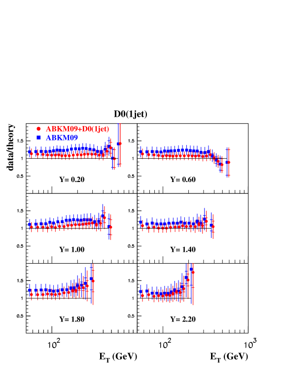

The hadronic jet production is sensitive to all nucleon PDFs, in particular to the large- gluon distribution, which is not sufficiently sensitive to other processes employed in PDF fits. Therefore the inclusive jet production data obtained by the Tevatron collider experiments [107, 105] are used in the PDF fits of [22, 24, 99] in order to provide better constraints on the large- gluon. The calculation of the full NNLO QCD corrections to this process is still in progress (see [205, 206] and references therein). This precludes a consistent use of the Tevatron jet data in our NNLO PDF fit. Nevertheless in order to check any potential impact of the jet Tevatron data on our PDFs we have performed trial variants of the NNLO ABKM09 fit with the Tevatron jet data added [102]. The NLO QCD corrections [207, 208] and the partial (soft gluon enhanced) NNLO corrections due to threshold resummation [109] have been computed with the FastNLO tool [209, 210].
In order to allow more flexibility of the large- gluon distribution we have added the term to the polynomial of eq. (4.9) with an additional fitted parameter making sure that further expansions of this polynomial do not improve the quality of those fits. In general, the Tevatron jet data overshoot the ABKM09 predictions, nevertheless they can be smoothly accommodated in the fit. The typical value of is achieved with account of the error correlations for the jet data sets of [107, 108, 105, 106] once they are included into the NNLO ABKM09 fit. Meanwhile the various data sets demonstrate a somewhat different trend with respect to the ABKM09 predictions. E.g., the off-set of the D0 inclusive jet data [107] does not depend on the jet energy and therefore may be attributed to the impact of the currently missing full NNLO corrections, cf. Figs. 5.2 and 5.3. In contrast, for the CDF data of [105] obtained with the jet algorithm the pulls rise with and can be reduced only by means of a modification of the PDF shapes.
| ABKM09 | D0 1-jet inc. | D0 di-jet | CDF 1-jet inc. | CDF 1-jet inc. | |
|---|---|---|---|---|---|
| (cone) | () | ||||
| Tevatron(1.96) | 0.770(50) | 0.859(29) | 0.833(27) | 0.815(25) | 0.842(25) |
| LHC(7) | 14.34(41) | 14.68(29) | 14.69(27) | 14.11(28) | 14.44(27) |
The values of extracted from the trial ABKM09 fits with the Tevatron jet data included are compared with the nominal ABKM09 value in Tab. 4.5. At most, they are bigger by 1, while for the CDF cone jet algorithm data [106] the central value of is even the same. A recent evaluation of using the ATLAS inclusive jet cross section data yields at NLO [211]. The predictions for the light Higgs production cross section, which are defined by the gluon distribution at , are also not very sensitive to the constraints coming from the Tevatron data, cf. Tab. 5.12. The impact of the Tevatron jet data on the large- gluon distribution is more significant. However, in this context we note that the Tevatron dijet and 3-jet production data are in good agreement with the ABKM09 predictions [212], in contrast to the case of inclusive jet production at Tevatron. The analysis of Tevatron data 3-jet production has also shown, that the predictions of MSTW [22] agree even better with the data of [213] than ABKM09. However, for the case of CT10 [24] this is opposite.
The trend of the first LHC data on the jet production with respect to the various PDF predictions is different from the Tevatron measurements. The ABKM09 predictions are in better agreement with the CMS and ATLAS inclusive data of [113, 214] than the predictions based on the PDFs of [22, 24, 99], which were tuned to the Tevatron inclusive jet data. In Figs. 5.4 and 5.5 we show a comparison of the result of the present fit and of MSTW [22] with LHC jet data from ATLAS [214] and from CMS [215] calculated with the updated version of the FastNLO code [210]. The trend of these data in comparison the predictions is the same for both experiments. We find good agreement at large transverse energy and small rapidity . The predictions overshoot the data for , i.e., in a range where the theory description is evidently incomplete. The predictions also overshoot the data (within the errors) at large . In summary this is the opposite trend as compared to the Tevatron data. If included in the PDF analysis and taking only data with say, the LHC jet data may potentially lead to a decrease of the large- gluons. This said, it should be kept in mind that jet data from the LHC is still subject to large systematic errors, though. In summary, these ambiguities in the data as well as the limitations in the current theoretical treatment prevent the use of hadronic jet data in our fit.

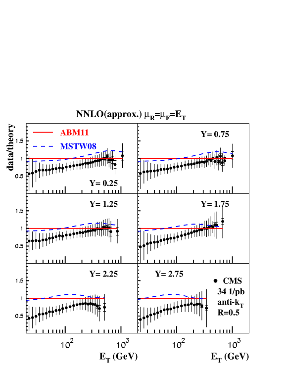
Finally let us also comment on [28] in this context which has studied the compatibility of the Tevatron jet data with the predictions based on the PDFs of ABKM09 [16] (see also [102]). The particular focus of [28] has been on shifts in the normalization uncertainty of the experimental data. Unfortunately, the study of [28] overestimates the statistical significance of such shifts in the normalization errors, since the PDF errors in the ABKM09 PDF sets have not been taken into account. The latter however should have a significant impact on the comparison because the large- gluon PDF of ABKM09, which is most relevant for such comparisons to Tevatron jet data, carries quite a large uncertainty in itself. This is corroborated by the fact that the value of obtained in the variants of the ABKM09 fit with the Tevatron data included [102] are quite good, illustrating in an indirect manner the irrelevance of [28].
5.5 LHAPDF library
For the cross section computations presented here we have used the LHAPDF library [216, 217] to interface to our PDFs and to those of other groups. For wider public use and to facilitate cross section computations by the interested reader, we provide the results of the current analysis in the form of data grids accessible with the most recent version lhapdf-5.8.7 of the LHAPDF library, which can be obtained from http://projects.hepforge.org/lhapdf. Please follow the instructions in the LHAPDF package to install the LHAPDF library.
In detail, we provide three NLO grids for flavors,
      abm11_3n_nlo.LHgrid (0+28),
      abm11_4n_nlo.LHgrid (0+28),
      abm11_5n_nlo.LHgrid (0+28),
with the central fit and 28 additional sets for the combined symmetric uncertainty on the PDFs and on from eqs. (4.12), (4.13), the heavy-quark masses from eq. (4.15), and the deuteron correction, cf. Fig. 2.1. Likewise at NNLO, we have
      abm11_3n_nnlo.LHgrid (0+28),
      abm11_4n_nnlo.LHgrid (0+28),
      abm11_5n_nnlo.LHgrid (0+28).
For future measurements of the strong coupling constant, e.g., from data on hadronic jet production as well as for detailed phenomenological studies of the parametric dependence of observables on , we also provide grids with fixed values of , see the discussion in Sec. 4.2. At NLO these are 20 sets in the range and at NNLO 16 sets for , cf. also Fig. 4.16. The sets for the scan are denoted
  abm11_5n_as_nlo.LHgrid (0+20),
  abm11_5n_as_nnlo.LHgrid (0+16).
During the computation of the cross sections with the LHAPDF library we have noticed significant differences in the run-time of our programs, when determining the cross section value and its uncertainty for a particular PDF set. Usually, this requires sampling of the error PDFs which describe the error of the corresponding parameter in a given set. The run-time, of course, depends on the number of parameters in a given set, but also on the parametrization of the PDF grid and details of the look-up algorithm. Efficiency for phenomenological studies requires sufficiently precise and at same time fast cross section computations.
Interestingly, for all observables discussed above, we have found the same pattern for the required run-times. The grids of ABKM09 [16] and ABM11 are both equally fast, i.e., . Next come the JR09 [20, 21] grids which are slightly slower by roughly a factor followed by the grids of MSTW [22] with . The grids of NN21 [23] are last in this row with run-times up by roughly a factor of five, . This is correlated with the enormous size of the latter grids of MByte for NN21 with 100 PDF sets, as compared, e.g., to the size of MByte for ABM11 or to MByte for MSTW. Note that the NN21 grids with 1000 PDF sets have a size of about GByte and typical run times up by another order of magnitude, making PDF error computations even more inefficient.
6 Conclusions
We have presented the PDF set ABM11 which determines the parton content of the nucleon and measures at NNLO accuracy in QCD. In order to achieve a description of our analysis which is as complete and as transparent possible, we have provided an extensive discussion of all ingredients. This begins with the theoretical foundations which are most advanced and (almost) fully consistent at NNLO in QCD using well-defined renormalization schemes for all parameters involved. We have given detailed information on our treatment of the additional higher twist terms and nuclear corrections as well as on all data sets involved and on our fit ansatz. The results presented have been exposed to numerous consistency checks to test stability and the statistical quality.
We have found good agreement with our previous results in ABKM09 and the PDF sets of ABM11 are readily available with the LHAPDF library for precision phenomenology at the LHC and other hadron colliders. We have studied the differences with respect to other PDF groups using the code OPENQCDRAD for standardized precision comparison. In this way some of the differences with respect to other PDF sets could be explained. The observed differences in the gluon PDFs are clearly outstanding in this context. This has important implications for the Higgs boson searches at the LHC and requires urgently further studies. In our present fit, thanks to OPENQCDRAD, we have provided a framework in which such questions can be addressed in the future.
Despite the fact that various extractions of have reached an impressive level of precision of 1%, there exist still larger systematic differences which depend on both, the particular observable under consideration as well as on the specific analysis carried out for a given observables (if compared to other analyses of the same observable). We have tried to analyse the status of the measurement of from world DIS data and the effect of including other hard scattering data. At present we feel, that not all data used in global analyses are of sufficient quality, considering the precision currently envisaged for .
The differences of the present analysis with respect to other groups have to be clarified in the future by performing dedicated mutual comparisons addressing the data sets used in the analyses, details of the theoretical description as well as the data analysis. Here an important issue concerns the systematics of different data sets. In some cases the analyses show tensions and it is even known from the experimental analyses themselves that significant differences exist which are of systematic nature. It is a rather delicate matter how to deal with those data in rather refined analyses at the precision of the NNLO level in QCD. These effects are partly responsible for the different results presently obtained in PDF fits of various groups. In the future, this situation can be significantly improved by (i) the availability of NNLO QCD corrections to hard jet cross sections; (ii) hard multi-jet data from the LHC with well-controlled systematics and within a wider energy range than available at Tevatron; (iii) precise and Drell-Yan data from the LHC. Gradually, also other hard scattering cross sections will be understood to NNLO and allow to constrain the PDFs much further.
It is therefore clear that the simplest way to reduce PDF uncertainties is not to discard non-global sets. Rather, it consists of very detailed studies of data sets, using the most complete theoretical descriptions, following D. Hilbert’s request: “Wir müssen wissen - wir werden wissen!” [218]. Precision QCD analyses will always refer to compatible sets of precise data with a detailed account of the systematic errors and all known theoretical corrections, which allows to measure all non-perturbative PDF parameters and the strong coupling constant as precisely as possible.
The QCD corrections are of vital importance to understand the production mechanism of new states as detailed as possible. In particular, the anticipated signal of a Higgs boson at a mass [219] has to be measured to highest precision. The aim of further PDF analyses has to consist in extracting both the gluon PDF and at even higher statistical and systematic precision because the dominant Higgs production in ggF behaves as and it is well-known that even the NNLO QCD corrections in ggF contribute a numerically significant portion to the total cross section. Also various other discoveries at hadron colliders may crucially depend on the thorough and precise understanding of the PDFs and QCD at high-energy scales.
Note added:
In the present analysis the comparison to NN21 has been carried out with the help of the grid NNPDF21_FFN3_100 in the LHAPDF repository dating from Aug 02, 2011. After publication of this article the grids of NN21 have been replaced and Figs. 4.10 and 4.21 have been updated with the grid NNPDF21_FFN3_100 now dating from Feb 17, 2012. With this new grid our conclusions remain unchanged.
Acknowledgments
We thank J. Baglio, H. Böttcher, S. Dinter, A. Djouadi, V. Drach, P. Jimenez-Delgado, E. Reya, and R. Thorne for discussions. We are thankful to V. Drach for preparing the plot in Fig. 4.23, to R. Thorne for providing us with the corresponding NLO plots not contained in [159] and to M. Zaro for computing the cross sections in Tab. 5.6. We also gratefully acknowledge the support of M. Whalley to integrate the results of the ABM11 fit into the LHAPDF library [216, 217].
J.B. acknowledges support from Technische Universität Dortmund. This work has been supported by Helmholtz Gemeinschaft under contract VH-HA-101 (Alliance Physics at the Terascale), by the Deutsche Forschungsgemeinschaft in Sonderforschungsbereich/Transregio 9 and by the European Commission through contract PITN-GA-2010-264564 (LHCPhenoNet).
Appendix A Statistics
A.1 Statistical procedures
In our analysis we infer the vector of fitted parameters from the experimental data minimizing the functional
| (A.1) |
where is the fitted model, are the measurements, and is the measurement error matrix with the indexes running through all data points included into the fit. The error matrix is the inverse of the covariance matrix . If the data are uncorrelated the covariance matrix is diagonal and
| (A.2) |
where are uncorrelated errors in the measurements . If, in addition, the data are subject to the point-to-point correlated systematic fluctuations, the off-diagonal terms appear in the covariance matrix as well. For counting experiments the systematic errors are commonly multiplicative. Therefore the general form of the covariance matrix employed in our analysis reads
| (A.3) |
where is the relative correlated systematic error in the measurement . The uncorrelated errors may stem both from the statistical and systematic uncertainties. In the later case they are combined with the statistical ones in quadrature to obtain . The estimator based on the functional of eq. (A.1) is statistically efficient and asymptotically unbiased in the limit of . In case of the analysis of correlated data the fitted parameters may be biased [220], however for the definition of eq. (A.3) the estimator is nevertheless asymptotically unbiased [221]. The errors in the fitted parameters given in Tab. 4.1 and the correlations coefficients of Tabs. A.1–A.3 are propagated from the uncertainties in the data with account of the correlations in the latter and correspond to the standard statistical criterion . The errors in the data normalization factors for the selected experiments, cf. Tabs. 3.1 and 3.2, which were fitted simultaneously with other parameters, are calculated in the same way.
The detailed information on the experimental uncertainities in all data sets considered in the fit and listed in Sec. 3 are available from http://arxiv.org as an attachment to the arXiv version of our paper. This includes in particular the systematic errors in the SLAC data [222] discussed in Sec. 3.1 and, likewise, the systematic errors in the NuTeV data and the corrections on the unmeasured phase space for the NuTeV and the CCFR data [223] discussed in Sec. 3.3.
A.2 Parameter correlation matrix
Here, we finally present the covariance matrix for the correlations of the fit parameters of ABM11 discussed in Sec. 4, cf. Tab. 4.1 and eq. (4.10) for and . The strong coupling is given in eq. (4.13), while in Tabs. A.1–A.3 we quote the correlations for with .
The correlations matrices for all other variants of the PDF fit discussed in the paper, e.g. those fits in Sec. 5.4 including Tevatron jet data are omitted for the brevity. However they are available from the authors upon request.
| 1.0000 | 0.9692 | 0.9787 | -0.7929 | 0.7194 | 0.5279 | -0.1460 | -0.1007 | 0.7481 | 0.6835 | -0.4236 | -0.2963 | 0.3391 | 0.3761 | |
| 1.0000 | 0.9396 | -0.7244 | 0.6792 | 0.4939 | -0.1146 | -0.1099 | 0.7404 | 0.6840 | -0.4146 | -0.3138 | 0.3464 | 0.3738 | ||
| 1.0000 | -0.8940 | 0.6506 | 0.4646 | -0.1865 | -0.0539 | 0.6728 | 0.6093 | -0.4799 | -0.2755 | 0.3441 | 0.3717 | |||
| 1.0000 | -0.4102 | -0.2267 | 0.2357 | -0.0182 | -0.4075 | -0.3495 | 0.4543 | 0.1713 | -0.3156 | -0.3149 | ||||
| 1.0000 | 0.8827 | -0.2155 | -0.1964 | 0.6875 | 0.6435 | -0.3030 | -0.3354 | 0.2635 | 0.3500 | |||||
| 1.0000 | -0.2462 | -0.0979 | 0.5359 | 0.5099 | -0.2957 | -0.3443 | 0.3157 | 0.3763 | ||||||
| 1.0000 | -0.2068 | -0.0689 | -0.0698 | 0.2381 | -0.0168 | 0.0384 | 0.0453 | |||||||
| 1.0000 | 0.1015 | 0.1279 | -0.4146 | -0.0852 | -0.1185 | -0.0892 | ||||||||
| 1.0000 | 0.9884 | -0.4678 | -0.4679 | 0.1961 | 0.2504 | |||||||||
| 1.0000 | -0.4520 | -0.5195 | 0.1982 | 0.2596 | ||||||||||
| 1.0000 | 0.1436 | 0.0444 | -0.0180 | |||||||||||
| 1.0000 | -0.6289 | -0.7662 | ||||||||||||
| 1.0000 | 0.9392 | |||||||||||||
| 1.0000 |
| -0.0435 | 0.0000 | -0.8480 | 0.6008 | 0.1535 | -0.0034 | -0.0437 | -0.0355 | 0.8111 | 0.0796 | -0.4797 | 0.0044 | -0.1718 | |
| -0.1251 | 0.0316 | -0.8375 | 0.5537 | 0.1806 | 0.0008 | -0.0345 | -0.0276 | 0.7001 | 0.0625 | -0.4889 | -0.0005 | -0.1452 | |
| -0.0849 | -0.0637 | -0.8133 | 0.5422 | 0.1667 | -0.0324 | -0.0671 | -0.0638 | 0.8948 | 0.0726 | -0.4033 | 0.0075 | -0.2028 | |
| 0.0920 | 0.1659 | 0.5760 | -0.3308 | -0.2276 | 0.0799 | 0.0966 | 0.1098 | -0.9749 | -0.0631 | 0.1728 | -0.0142 | 0.2353 | |
| -0.0321 | -0.0137 | -0.7618 | 0.9630 | -0.1842 | 0.0007 | -0.0414 | -0.0167 | 0.4878 | 0.0227 | -0.4735 | -0.0078 | -0.2088 | |
| -0.1666 | -0.1167 | -0.6060 | 0.9351 | -0.5969 | -0.0064 | -0.0249 | -0.0203 | 0.3007 | -0.0045 | -0.3782 | -0.0132 | -0.2121 | |
| 0.0206 | 0.8718 | 0.1649 | -0.2544 | 0.1916 | -0.0232 | -0.0212 | -0.0294 | -0.2398 | 0.0202 | 0.0667 | 0.0034 | 0.9721 | |
| 0.0086 | -0.6291 | -0.1067 | -0.1834 | -0.1103 | 0.0594 | 0.0577 | 0.0711 | 0.0052 | -0.0063 | -0.1768 | -0.0083 | -0.0662 | |
| 0.0043 | -0.0481 | -0.8662 | 0.5862 | 0.0768 | -0.0341 | -0.0659 | -0.0493 | 0.4485 | 0.1559 | -0.8164 | -0.0008 | -0.0417 | |
| -0.0459 | -0.0650 | -0.8255 | 0.5493 | 0.0606 | -0.0119 | -0.0441 | -0.0255 | 0.3870 | 0.0940 | -0.8628 | -0.0055 | -0.0375 | |
| -0.0382 | 0.3783 | 0.7032 | -0.3288 | 0.1278 | -0.0734 | -0.0445 | -0.0807 | -0.4262 | -0.0100 | 0.3911 | 0.0040 | 0.1782 | |
| 0.3785 | 0.0061 | 0.3050 | -0.3280 | 0.1338 | 0.0936 | 0.0718 | 0.1165 | -0.1744 | -0.0137 | 0.4886 | 0.0323 | -0.0360 | |
| -0.6085 | 0.1017 | -0.0873 | 0.2827 | -0.2104 | -0.0543 | -0.0114 | -0.1223 | 0.2973 | 0.1560 | -0.1337 | 0.0141 | 0.0066 | |
| -0.4642 | 0.1021 | -0.1778 | 0.3605 | -0.1962 | -0.0708 | -0.0396 | -0.1230 | 0.3132 | 0.0425 | -0.1977 | 0.0071 | 0.0201 |
| 1.0000 | 0.0176 | -0.0394 | -0.0798 | 0.2357 | -0.0018 | -0.0982 | -0.0075 | -0.0291 | 0.1904 | 0.0676 | 0.0562 | 0.0136 | |
| 1.0000 | 0.1183 | -0.0802 | 0.2640 | -0.0427 | -0.0489 | -0.0550 | -0.1595 | 0.0193 | 0.0985 | 0.0069 | 0.7657 | ||
| 1.0000 | -0.6753 | -0.0493 | -0.0525 | 0.0158 | -0.0445 | -0.6039 | -0.0656 | 0.6590 | 0.0017 | 0.1487 | |||
| 1.0000 | -0.4041 | -0.0213 | -0.0513 | -0.0366 | 0.4145 | 0.0148 | -0.3931 | -0.0086 | -0.2284 | ||||
| 1.0000 | 0.0308 | -0.0016 | 0.0326 | 0.1801 | 0.0276 | -0.0510 | 0.0111 | 0.1212 | |||||
| 1.0000 | 0.8570 | 0.9749 | -0.0664 | -0.0206 | -0.4355 | 0.0017 | -0.0139 | ||||||
| 1.0000 | 0.8730 | -0.0894 | -0.0706 | -0.3708 | 0.0005 | -0.0127 | |||||||
| 1.0000 | -0.0967 | -0.1234 | -0.4403 | -0.0050 | -0.0172 | ||||||||
| 1.0000 | 0.0674 | -0.2082 | 0.0153 | -0.2378 | |||||||||
| 1.0000 | -0.0010 | 0.0505 | 0.0141 | ||||||||||
| 1.0000 | 0.0083 | 0.0276 | |||||||||||
| 1.0000 | 0.0006 | ||||||||||||
| 1.0000 |
References
- [1] S. Alekhin, Phys.Lett. B519, 57 (2001), hep-ph/0107197.
- [2] S. Moch, J. Vermaseren, and A. Vogt, Nucl.Phys. B688, 101 (2004), hep-ph/0403192.
- [3] A. Vogt, S. Moch, and J. Vermaseren, Nucl.Phys. B691, 129 (2004), hep-ph/0404111.
- [4] W. van Neerven and E. Zijlstra, Phys.Lett. B272, 127 (1991).
- [5] E. Zijlstra and W. van Neerven, Phys.Lett. B273, 476 (1991).
- [6] E. Zijlstra and W. van Neerven, Nucl.Phys. B383, 525 (1992).
- [7] E. Zijlstra and W. van Neerven, Phys.Lett. B297, 377 (1992).
- [8] S. Moch and J. Vermaseren, Nucl.Phys. B573, 853 (2000), hep-ph/9912355.
- [9] S. Moch, J. Vermaseren, and A. Vogt, Phys.Lett. B606, 123 (2005), hep-ph/0411112.
- [10] J. Vermaseren, A. Vogt, and S. Moch, Nucl.Phys. B724, 3 (2005), hep-ph/0504242.
- [11] R. Hamberg, W. van Neerven, and T. Matsuura, Nucl.Phys. B359, 343 (1991).
- [12] R. V. Harlander and W. B. Kilgore, Phys.Rev.Lett. 88, 201801 (2002), hep-ph/0201206.
- [13] C. Anastasiou, L. J. Dixon, K. Melnikov, and F. Petriello, Phys.Rev.Lett. 91, 182002 (2003), hep-ph/0306192.
- [14] C. Anastasiou, L. J. Dixon, K. Melnikov, and F. Petriello, Phys.Rev. D69, 094008 (2004), hep-ph/0312266.
- [15] S. Catani, L. Cieri, G. Ferrera, D. de Florian, and M. Grazzini, Phys.Rev.Lett. 103, 082001 (2009), arXiv:0903.2120.
- [16] S. Alekhin, J. Blümlein, S. Klein, and S. Moch, Phys.Rev. D81, 014032 (2010), arXiv:0908.2766.
- [17] S. Alekhin, J. Blümlein, and S. Moch, PoS DIS2010, 021 (2010), arXiv:1007.3657.
- [18] H1 and ZEUS Collaboration, F. Aaron et al., JHEP 1001, 109 (2010), arXiv:0911.0884.
- [19] HERAPDF, https://www.desy.de/h1zeus/combined_results/index.php?do=proton_structure.
- [20] P. Jimenez-Delgado and E. Reya, Phys.Rev. D79, 074023 (2009), arXiv:0810.4274.
- [21] P. Jimenez-Delgado and E. Reya, Phys.Rev. D80, 114011 (2009), arXiv:0909.1711.
- [22] A. Martin, W. Stirling, R. Thorne, and G. Watt, Eur.Phys.J. C63, 189 (2009), arXiv:0901.0002.
- [23] R. D. Ball et al., Nucl.Phys. B855, 153 (2012), arXiv:1107.2652.
- [24] H.-L. Lai et al., Phys.Rev. D82, 074024 (2010), arXiv:1007.2241.
- [25] J. Baglio and A. Djouadi, JHEP 1010, 064 (2010), arXiv:1003.4266.
- [26] S. Alekhin, J. Blümlein, P. Jimenez-Delgado, S. Moch, and E. Reya, Phys. Lett. B697, 127 (2011), arXiv:1011.6259.
- [27] S. Alekhin, J. Blümlein, and S. Moch, Eur. Phys. J. C71, 1723 (2011), arXiv:1101.5261.
- [28] R. Thorne and G. Watt, JHEP 1108, 100 (2011), arXiv:1106.5789.
- [29] G. Watt, JHEP 1109, 069 (2011), arXiv:1106.5788.
- [30] R. D. Ball et al., Phys.Lett. B704, 36 (2011), arXiv:1102.3182.
- [31] H1 Collaboration, F. Aaron et al., Eur.Phys.J. C71, 1579 (2011), arXiv:1012.4355.
- [32] S. Alekhin and S. Moch, Phys.Lett. B699, 345 (2011), arXiv:1011.5790.
- [33] A. Vogt, Comput.Phys.Commun. 170, 65 (2005), hep-ph/0408244.
- [34] G. P. Salam and J. Rojo, Comput.Phys.Commun. 180, 120 (2009), arXiv:0804.3755.
- [35] S. Moch, J. Vermaseren, and A. Vogt, Nucl.Phys. B813, 220 (2009), arXiv:0812.4168.
- [36] E. Laenen, S. Riemersma, J. Smith, and W. van Neerven, Nucl. Phys. B392, 162 (1993).
- [37] T. Gottschalk, Phys.Rev. D23, 56 (1981).
- [38] M. Glück, S. Kretzer, and E. Reya, Phys.Lett. B380, 171 (1996), hep-ph/9603304.
- [39] E. Laenen and S. Moch, Phys. Rev. D59, 034027 (1999), hep-ph/9809550.
- [40] S. Alekhin and S. Moch, Phys. Lett. B672, 166 (2009), arXiv:0811.1412.
- [41] N. Presti, H. Kawamura, S. Moch, and A. Vogt, PoS DIS2010, 163 (2010), arXiv:1008.0951.
- [42] G. Corcella and A. D. Mitov, Nucl.Phys. B676, 346 (2004), hep-ph/0308105.
- [43] M. Buza, Y. Matiounine, J. Smith, R. Migneron, and W. van Neerven, Nucl.Phys. B472, 611 (1996), hep-ph/9601302.
- [44] M. Buza, Y. Matiounine, J. Smith, and W. van Neerven, Eur.Phys.J. C1, 301 (1998), hep-ph/9612398.
- [45] I. Bierenbaum, J. Blümlein, and S. Klein, Nucl.Phys. B780, 40 (2007), hep-ph/0703285.
- [46] I. Bierenbaum, J. Blumlein, and S. Klein, Phys.Lett. B672, 401 (2009), arXiv:0901.0669.
- [47] I. Bierenbaum, J. Blümlein, and S. Klein, Nucl.Phys. B820, 417 (2009), arXiv:0904.3563.
- [48] J. Ablinger, J. Blümlein, S. Klein, C. Schneider, and F. Wissbrock, Nucl.Phys. B844, 26 (2011), arXiv:1008.3347.
- [49] S. Alekhin and J. Blümlein, Phys.Lett. B594, 299 (2004), hep-ph/0404034.
- [50] J. Blümlein, A. Hasselhuhn, P. Kovacikova, and S. Moch, Phys.Lett. B700, 294 (2011), arXiv:1104.3449.
- [51] S. Larin, T. van Ritbergen, and J. Vermaseren, Nucl.Phys. B438, 278 (1995), hep-ph/9411260.
- [52] K. Chetyrkin, B. A. Kniehl, and M. Steinhauser, Phys.Rev.Lett. 79, 2184 (1997), hep-ph/9706430.
- [53] OPENQCDRAD, http://www-zeuthen.desy.de/~alekhin/OPENQCDRAD .
- [54] A. Martin, R. Roberts, W. Stirling, and R. Thorne, Eur.Phys.J. C39, 155 (2005), hep-ph/0411040.
- [55] S. Moch, J. Vermaseren, and A. Vogt, Nucl.Phys. B621, 413 (2002), hep-ph/0110331.
- [56] A. Vogt, S. Moch, and J. Vermaseren, Acta Phys.Polon. B37, 683 (2006), hep-ph/0511112.
- [57] H. Georgi and H. Politzer, Phys.Rev. D14, 1829 (1976).
- [58] O. Nachtmann, Nucl.Phys. B63, 237 (1973).
- [59] M. Virchaux and A. Milsztajn, Phys.Lett. B274, 221 (1992).
- [60] J. Blümlein, H. Böttcher, and A. Guffanti, Nucl.Phys. B774, 182 (2007), hep-ph/0607200.
- [61] J. Blümlein and H. Böttcher, Phys.Lett. B662, 336 (2008), arXiv:0802.0408.
- [62] L. Whitlow, S. Rock, A. Bodek, E. Riordan, and S. Dasu, Phys.Lett. B250, 193 (1990).
- [63] E. V. Shuryak and A. Vainshtein, Nucl.Phys. B199, 451 (1982).
- [64] S. Alekhin, Phys.Rev. D63, 094022 (2001), hep-ph/0011002.
- [65] V. Braun, A. Manashov, and J. Rohrwild, Nucl.Phys. B826, 235 (2010), arXiv:0908.1684.
- [66] S. Alekhin, S. A. Kulagin, and R. Petti, AIP Conf.Proc. 967, 215 (2007), arXiv:0710.0124.
- [67] S. Alekhin, S. A. Kulagin, and S. Liuti, Phys.Rev. D69, 114009 (2004), hep-ph/0304210.
- [68] S. Alekhin, S. A. Kulagin, and R. Petti, Phys.Lett. B675, 433 (2009), arXiv:0812.4448.
- [69] S. Alekhin, S. A. Kulagin, and R. Petti, (2008), arXiv:0810.4893.
- [70] S. A. Kulagin and R. Petti, Nucl.Phys. A765, 126 (2006), hep-ph/0412425.
- [71] J. Arrington, J. Rubin, and W. Melnitchouk, (2011), arXiv:1110.3362.
- [72] S. Kulagin and R. Petti, Phys.Rev. C82, 054614 (2010), arXiv:1004.3062.
- [73] M. Lacombe et al., Phys.Rev. C21, 861 (1980).
- [74] R. Machleidt, K. Holinde, and C. Elster, Phys.Rept. 149, 1 (1987).
- [75] S. A. Kulagin and R. Petti, Phys.Rev. D76, 094023 (2007), hep-ph/0703033.
- [76] D. Alde et al., Phys.Rev.Lett. 64, 2479 (1990).
- [77] A. Bodek et al., Phys.Rev. D20, 1471 (1979).
- [78] W. Atwood et al., Phys.Lett. B64, 479 (1976).
- [79] M. Mestayer et al., Phys.Rev. D27, 285 (1983).
- [80] J. Gomez et al., Phys.Rev. D49, 4348 (1994).
- [81] S. Dasu et al., Phys.Rev. D49, 5641 (1994).
- [82] BCDMS Collaboration, A. Benvenuti et al., Phys.Lett. B223, 485 (1989).
- [83] BCDMS Collaboration, A. Benvenuti et al., Phys.Lett. B237, 592 (1990).
- [84] NMC Collaboration, M. Arneodo et al., Nucl.Phys. B483, 3 (1997), hep-ph/9610231.
- [85] A. Arbuzov, D. Y. Bardin, J. Blümlein, L. Kalinovskaya, and T. Riemann, Comput.Phys.Commun. 94, 128 (1996), hep-ph/9511434.
- [86] H1 Collaboration, C. Adloff et al., Eur.Phys.J. C21, 33 (2001), hep-ex/0012053.
- [87] ZEUS Collaboration, S. Chekanov et al., Eur.Phys.J. C21, 443 (2001), hep-ex/0105090.
- [88] NMC Collaboration., M. Arneodo et al., Phys.Lett. B364, 107 (1995), hep-ph/9509406.
- [89] L. Whitlow, (1990), Ph.D. Thesis.
- [90] G. Moreno et al., Phys.Rev. D43, 2815 (1991).
- [91] FNAL E866/NuSea Collaboration, R. Towell et al., Phys.Rev. D64, 052002 (2001), hep-ex/0103030.
- [92] NuSea Collaboration, J. Webb et al., Phys.Rev.Lett. (2003), hep-ex/0302019.
- [93] S. Alekhin, K. Melnikov, and F. Petriello, Phys.Rev. D74, 054033 (2006), hep-ph/0606237.
- [94] CCFR Collaboration, A. Bazarko et al., Z.Phys. C65, 189 (1995), hep-ex/9406007.
- [95] NuTeV Collaboration, M. Goncharov et al., Phys.Rev. D64, 112006 (2001), hep-ex/0102049.
- [96] D. A. Mason, (2006), Ph.D. Thesis (Advisor: Raymond E. Frey).
- [97] S. Alekhin, J. Blümlein, H. Böttcher, and S. Moch, (2011), arXiv:1104.0469.
- [98] Particle Data Group, K. Nakamura et al., J.Phys.G G37, 075021 (2010).
- [99] R. D. Ball et al., Nucl.Phys. B849, 296 (2011), arXiv:1101.1300.
- [100] Jefferson Lab E00-115 Collaboration, S. Malace et al., Phys.Rev. C80, 035207 (2009), arXiv:0905.2374.
- [101] J. Sanchez Guillen, J. Miramontes, M. Miramontes, G. Parente, and O. Sampayo, Nucl.Phys. B353, 337 (1991).
- [102] S. Alekhin, J. Blümlein, and S. Moch, (2011), arXiv:1105.5349.
- [103] New Muon Collaboration, M. Arneodo et al., Phys.Lett. B309, 222 (1993).
- [104] D0 Collaboration, V. M. Abazov et al., Phys. Rev. D80, 111107 (2009), arXiv:0911.2710.
- [105] CDF - Run II, A. Abulencia et al., Phys.Rev. D75, 092006 (2007), hep-ex/0701051.
- [106] CDF Collaboration, T. Aaltonen et al., Phys.Rev. D78, 052006 (2008), arXiv:0807.2204.
- [107] D0 Collaboration, V. Abazov et al., Phys.Rev.Lett. 101, 062001 (2008), arXiv:0802.2400.
- [108] D0 Collaboration, V. Abazov et al., Phys.Lett. B693, 531 (2010), arXiv:1002.4594.
- [109] N. Kidonakis and J. Owens, Phys.Rev. D63, 054019 (2001), hep-ph/0007268.
- [110] J. Blümlein and H. Böttcher, arXiv:1207.3170.
- [111] J. Blümlein, S. Riemersma, W. van Neerven, and A. Vogt, Nucl.Phys.Proc.Suppl. 51C, 97 (1996), hep-ph/9609217.
- [112] CDF Collaboration, T. Affolder et al., Phys.Rev.Lett. 88, 042001 (2002), hep-ex/0108034.
- [113] K. Rabbertz, CERN Report No. CMS-NOTE-2011-004., 2011 (unpublished).
- [114] D0 and CDF Collaboration, D. Bandurin, (2011), arXiv:1112.0051.
- [115] R. Frederix, S. Frixione, K. Melnikov, and G. Zanderighi, JHEP 11, 050 (2010), arXiv:1008.5313.
- [116] B. Shaikhatdenov, A. Kotikov, V. Krivokhizhin, and G. Parente, Phys.Rev. D81, 034008 (2010), arXiv:0912.4672.
- [117] BCDMS Collaboration, A. Benvenuti et al., Phys.Lett. B223, 490 (1989).
- [118] BCDMS Collaboration, A. Benvenuti et al., Phys.Lett. B237, 599 (1990).
- [119] L. Whitlow, E. Riordan, S. Dasu, S. Rock, and A. Bodek, Phys.Lett. B282, 475 (1992).
- [120] P. A. Baikov and K. G. Chetyrkin, Nucl. Phys. Proc. Suppl. 160, 76 (2006).
- [121] V. Velizhanin, Nucl.Phys. B860, 288 (2012), arXiv:1112.3954.
- [122] S. Lionetti et al., Phys.Lett. B701, 346 (2011), arXiv:1103.2369.
- [123] R. D. Ball et al., Phys.Lett. B707, 66 (2012), arXiv:1110.2483.
- [124] New Muon Collaboration, M. Arneodo et al., Nucl.Phys. B487, 3 (1997), hep-ex/9611022.
- [125] ZEUS Collaboration, S. Chekanov et al., Eur.Phys.J. C61, 223 (2009), arXiv:0812.4620.
- [126] ZEUS Collaboration, S. Chekanov et al., Eur.Phys.J. C62, 625 (2009), arXiv:0901.2385.
- [127] ZEUS Collaboration, J. Breitweg et al., Eur.Phys.J. C12, 35 (2000), hep-ex/9908012.
- [128] ZEUS Collaboration, S. Chekanov et al., Phys.Rev. D69, 012004 (2004), hep-ex/0308068.
- [129] ZEUS Collaboration, S. Chekanov et al., Eur.Phys.J. C63, 171 (2009), arXiv:0812.3775.
- [130] ZEUS Collaboration, S. Chekanov et al., Eur.Phys.J. C65, 65 (2010), arXiv:0904.3487.
- [131] J. C. Webb, (2003), hep-ex/0301031, Ph.D. Thesis (Advisor: Vassili Papavassiliou).
- [132] CDF Collaboration, T. Aaltonen et al., Phys.Rev.Lett. 102, 181801 (2009), arXiv:0901.2169.
- [133] CDF Collaboration, T. A. Aaltonen et al., Phys.Lett. B692, 232 (2010), arXiv:0908.3914.
- [134] D0 Collaboration, V. Abazov et al., Phys.Rev. D76, 012003 (2007), hep-ex/0702025.
- [135] E665 Collaboration, M. R. Adams et al., Phys. Rev. D54, 3006 (1996).
- [136] NuTeV Collaboration, M. Tzanov et al., Phys. Rev. D74, 012008 (2006), hep-ex/0509010.
- [137] CHORUS Collaboration, G. Onengut et al., Phys. Lett. B632, 65 (2006).
- [138] E. M. Lobodzinska, (2003), hep-ph/0311180.
- [139] H1 Collaboration, C. Adloff et al., Eur. Phys. J. C30, 1 (2003), hep-ex/0304003.
- [140] H1 Collaboration, C. Adloff et al., Eur. Phys. J. C19, 269 (2001), hep-ex/0012052.
- [141] ZEUS Collaboration, J. Breitweg et al., Eur. Phys. J. C7, 609 (1999), hep-ex/9809005.
- [142] ZEUS Collaboration, S. Chekanov et al., Eur. Phys. J. C28, 175 (2003), hep-ex/0208040.
- [143] ZEUS Collaboration, S. Chekanov et al., Phys. Rev. D70, 052001 (2004), hep-ex/0401003.
- [144] ZEUS Collaboration, S. Chekanov et al., Eur. Phys. J. C32, 1 (2003), hep-ex/0307043.
- [145] H1 Collaboration, C. Adloff et al., Z. Phys. C72, 593 (1996), hep-ex/9607012.
- [146] H1 Collaboration, C. Adloff et al., Phys. Lett. B528, 199 (2002), hep-ex/0108039.
- [147] H1 Collaboration, A. Aktas et al., Eur.Phys.J. C45, 23 (2006), hep-ex/0507081.
- [148] H1 Collaboration, A. Aktas et al., Eur. Phys. J. C40, 349 (2005), hep-ex/0411046.
- [149] H1 Collaboration, F. D. Aaron et al., Eur. Phys. J. C65, 363 (2010), arXiv:0904.3870.
- [150] H1 Collaboration, A. Aktas et al., Phys. Lett. B653, 134 (2007), arXiv:0706.3722.
- [151] ZEUS Collaboration, ZEUS-prel-10-002.
- [152] ZEUS Collaboration, S. Chekanov et al., Phys. Lett. B547, 164 (2002), hep-ex/0208037.
- [153] ZEUS Collaboration, S. Chekanov et al., Nucl. Phys. B765, 1 (2007), hep-ex/0608048.
- [154] D0 Collaboration, V. M. Abazov et al., Phys. Rev. D77, 011106 (2008), arXiv:0709.4254.
- [155] CDF Collaboration, D. Acosta et al., Phys. Rev. D71, 051104 (2005), hep-ex/0501023.
- [156] CDF Collaboration, J. Han et al., public note, May 2008, http:www-cdf.fnal.gov/physics/ewk/2008/dszdy/.
- [157] G. Grindhammer, AIP Conf. Proc. 1441, 225 (2012), arXiv:1112.0224.
- [158] R. Kogler, Nucl. Phys. Proc. Suppl. 222-224, 81 (2012), arXiv:1112.5117.
- [159] A. D. Martin, W. J. Stirling, R. S. Thorne, and G. Watt, Eur. Phys. J. C64, 653 (2009), arXiv:0905.3531.
- [160] R. Thorne, private communication.
- [161] M. Glück, E. Reya, and C. Schuck, Nucl. Phys. B754, 178 (2006), hep-ph/0604116.
-
[162]
P. Nadolsky,
News from CTEQ-TEA PDF analysis, July 2011,
http://indico.desy.de/conferenceDisplay.py?confId=4211 (unpublished). - [163] T. Gehrmann, M. Jaquier, and G. Luisoni, Eur. Phys. J. C67, 57 (2010), arXiv:0911.2422.
- [164] R. Abbate, M. Fickinger, A. H. Hoang, V. Mateu, and I. W. Stewart, Phys. Rev. D83, 074021 (2011), arXiv:1006.3080.
- [165] G. Dissertori et al., Phys.Rev.Lett. 104, 072002 (2010), arXiv:0910.4283.
- [166] P. A. Baikov, K. G. Chetyrkin, and J. H. Kühn, Phys. Rev. Lett. 101, 012002 (2008), arXiv:0801.1821.
- [167] P. Baikov, K. Chetyrkin, J. Kühn, and J. Rittinger, Phys.Rev.Lett. 108, 222003 (2012), arXiv:1201.5804.
- [168] S. Bethke et al., (2011), arXiv:1110.0016.
- [169] D. Boito et al., Phys. Rev. D84, 113006 (2011), arXiv:1110.1127.
- [170] PACS-CS Collaboration, S. Aoki et al., JHEP 0910, 053 (2009), arXiv:0906.3906.
- [171] C. McNeile, C. T. H. Davies, E. Follana, K. Hornbostel, and G. P. Lepage, Phys. Rev. D82, 034512 (2010), arXiv:1004.4285.
- [172] B. Blossier et al., (2012), arXiv:1201.5770.
- [173] S. Bethke, Eur. Phys. J. C64, 689 (2009), arXiv:0908.1135.
- [174] R. Sommer, private communication.
- [175] H1 Collaboration, F. Aaron et al., Eur.Phys.J. C71, 1769 (2011), arXiv:1106.1028.
- [176] S. Alekhin and S. Moch, (2011), arXiv:1107.0469.
- [177] B. Harris and J. Smith, Nucl.Phys. B452, 109 (1995), hep-ph/9503484.
- [178] H1 and ZEUS Collaboration, H1prelim-10-143 and ZEUS-prel-10-019.
- [179] QCDSF/UKQCD Collaboration, D. Pleiter et al., PoS LATTICE2010, 153 (2010), arXiv:1101.2326.
- [180] Y. Aoki et al., Phys.Rev. D82, 014501 (2010), arXiv:1003.3387.
- [181] LHPC Collaboration, J. Bratt et al., Phys.Rev. D82, 094502 (2010), arXiv:1001.3620.
- [182] C. Alexandrou et al., Phys.Rev. D83, 114513 (2011), arXiv:1104.1600.
- [183] S. Dinter et al., PoS LATTICE2010, 135 (2010), arXiv:1101.5540.
- [184] S. Dinter et al., Phys.Lett. B704, 89 (2011), arXiv:1108.1076.
- [185] G. S. Bali et al., (2012), arXiv:1207.1110.
- [186] C. Anastasiou and K. Melnikov, Nucl.Phys. B646, 220 (2002), hep-ph/0207004.
- [187] V. Ravindran, J. Smith, and W. van Neerven, Nucl.Phys. B665, 325 (2003), hep-ph/0302135.
- [188] V. Ravindran, J. Smith, and W. van Neerven, Nucl.Phys. B704, 332 (2005), hep-ph/0408315.
- [189] P. Bolzoni, F. Maltoni, S. Moch, and M. Zaro, Phys.Rev.Lett. 105, 011801 (2010), arXiv:1003.4451.
- [190] P. Bolzoni, F. Maltoni, S. Moch, and M. Zaro, Phys. Rev. D85, 035002 (2012), arXiv:1109.3717.
- [191] O. Brein, A. Djouadi, and R. Harlander, Phys.Lett. B579, 149 (2004), hep-ph/0307206.
- [192] U. Langenfeld, S. Moch, and P. Uwer, Phys.Rev. D80, 054009 (2009), arXiv:0906.5273.
- [193] M. Aliev et al., Comput.Phys.Commun. 182, 1034 (2011), arXiv:1007.1327.
- [194] S. Catani, G. Ferrera, and M. Grazzini, JHEP 1005, 006 (2010), arXiv:1002.3115.
- [195] M. Glück, P. Jimenez-Delgado, E. Reya, and C. Schuck, Phys.Lett. B664, 133 (2008), arXiv:0801.3618.
- [196] ATLAS Collaboration, G. Aad et al., Phys.Lett. B701, 31 (2011), arXiv:1103.2929.
- [197] CMS Collaboration, S. Chatrchyan et al., JHEP 1104, 050 (2011), arXiv:1103.3470.
- [198] R. Gavin, Y. Li, F. Petriello, and S. Quackenbush, Comput.Phys.Commun. 182, 2388 (2011), arXiv:1011.3540.
- [199] Y. Amhis (for the LHCb Collaboration), (2012), arXiv:1202.0654.
- [200] S. Moch and A. Vogt, Phys.Lett. B631, 48 (2005), hep-ph/0508265.
- [201] G. Ferrera, M. Grazzini, and F. Tramontano, Phys.Rev.Lett. 107, 152003 (2011), arXiv:1107.1164.
- [202] B. A. Kniehl, Phys.Rev. D42, 2253 (1990).
- [203] O. Brein, R. Harlander, M. Wiesemann, and T. Zirke, (2011), arXiv:1111.0761.
- [204] D0 Collaboration, V. M. Abazov et al., Phys.Lett. B703, 422 (2011), arXiv:1104.2887.
- [205] A. Gehrmann-De Ridder, E. Glover, and J. Pires, (2011), arXiv:1112.3613.
- [206] P. Bolzoni, G. Somogyi, and Z. Trocsanyi, JHEP 1101, 059 (2011), arXiv:1011.1909.
- [207] Z. Nagy, Phys.Rev.Lett. 88, 122003 (2002), hep-ph/0110315.
- [208] Z. Nagy, Phys.Rev. D68, 094002 (2003), hep-ph/0307268.
- [209] T. Kluge, K. Rabbertz, and M. Wobisch, (2006), hep-ph/0609285.
- [210] M. Wobisch, D. Britzger, T. Kluge, K. Rabbertz, and F. Stober, (2011), arXiv:1109.1310.
- [211] B. Malaescu and P. Starovoitov, (2012), arXiv:1203.5416.
- [212] M. Wobisch, Nucl. Phys. Proc. Suppl. 222-224, 204 (2012), arXiv:1202.0205.
- [213] D0 Collaboration, V. M. Abazov et al., Phys.Lett. B704, 434 (2011), arXiv:1104.1986.
- [214] ATLAS Collaboration, G. Aad et al., (2011), arXiv:1112.6297.
- [215] CMS Collaboration, S. Chatrchyan et al. Phys.Rev.Lett. 107, 132001 (2011), arXiv:1106.0208.
- [216] M. Whalley, D. Bourilkov, and R. Group, (2005), hep-ph/0508110.
- [217] LHAPDF, http://hepforge.cedar.ac.uk/lhapdf/ .
- [218] D. Hilbert, Address to the Society of German Scientists and Physicians, at Königsberg, Sep. 8th, 1930.
-
[219]
ATLAS and CMS Collaborations,
Talks on the update of the Higgs-boson search, 4th July, 2012,
http://indico.cern.ch/conferenceDisplay.py?confId=197461. - [220] G. D’Agostini, Nucl.Instrum.Meth. A346, 306 (1994).
- [221] S. Alekhin, (2000), hep-ex/0005042.
- [222] L. Whitlow, private communication.
- [223] D. Mason, private communication.