Asteroid taxonomic signatures from photometric phase curves

Abstract

We explore the correlation between an asteroid’s taxonomy and photometric phase curve using the $H,\!G_{12}$ photometric phase function, with the shape of the phase function described by the single parameter $G_{12}$. We explore the usability of $G_{12}$ in taxonomic classification for individual objects, asteroid families, and dynamical groups. We conclude that the mean values of $G_{12}$ for the considered taxonomic complexes are statistically different, and also discuss the overall shape of the $G_{12}$ distribution for each taxonomic complex. Based on the values of $G_{12}$ for about half a million asteroids, we compute the probabilities of C, S, and X complex membership for each asteroid. For an individual asteroid, these probabilities are rather evenly distributed over all of the complexes, thus preventing meaningful classification. We then present and discuss the $G_{12}$ distributions for asteroid families, and predict the taxonomic complex preponderance for asteroid families given the distribution of $G_{12}$ in each family. For certain asteroid families, the probabilistic prediction of taxonomic complex preponderance can clearly be made. In particular, the C complex preponderant families are the easiest to detect, the Dora and Themis families being prime examples of such families. We continue by presenting the $G_{12}$-based distribution of taxonomic complexes throughout the main asteroid belt in the proper element phase space. The Nysa-Polana family shows two distinct regions in the proper element space with different $G_{12}$ values dominating in each region. We conclude that the $G_{12}$-based probabilistic distribution of taxonomic complexes through the main belt agrees with the general view of C complex asteroid proportion increasing towards the outer belt. We conclude that the $G_{12}$ photometric parameter cannot be used in determining taxonomic complex for individual asteroids, but it can be utilized in the statistical treatment of asteroid families and different regions of the main asteroid belt.

1 Introduction

The photometric phase function describes the relationship between the reduced magnitude (apparent magnitude at $1$ AU distance) and the solar phase angle (Sun-asteroid-observer angle). Previously in Oszkiewicz et al. (2011), we have fitted $H,\!G_{1},\!G_{2}$ and $H,\!G_{12}$ phase functions presented in Muinonen et al. (2010a) for about half a million asteroids contained in the Lowell Observatory database and obtained absolute magnitudes and photometric parameter(s) for each asteroid. The absolute magnitude $H$ for an asteroid is defined as the apparent $V$ band magnitude that the object would have if it were $1$ AU from both the Sun and the observer and at zero phase angle. The absolute magnitude relates directly to asteroid size and geometric albedo. The geometric albedo of an object is the ratio of its actual brightness at zero phase angle to that of an idealized Lambertian disk having the same cross-section.

The shape of the phase curve described by the $G_{1},\!G_{2}$ and $G_{12}$ parameters relates to the physical properties of an asteroid’s surface, such as geometric albedo, composition, porosity, roughness, and grain size distribution. For phase angles larger than 10^∘, steep phase curves are characteristic of low-albedo objects with an exposed regolith, whereas flat phase curves can indicate, for example, a high-albedo object with a substantial amount of multiple scattering in its regolith.

At small phase angles, atmosphereless bodies (such as asteroids) exhibit a pronounced nonlinear surge in apparent brightness known as the opposition effect (Muinonen et al., 2010b). The opposition effect was first recognized for asteroid (20) Massalia (Gehrels, 1955). The explanation of the opposition effect is two-fold: (1) self-shadowing arising in a rough and porous regolith, and (2) coherent backscattering; that is, constructive interference between two electromagnetic wave components propagating in opposite directions in the random medium (Muinonen et al., 2010b). The width and height of the opposition surge can suggest, for example, the compaction state of the regolith and the distribution of particle sizes.

Belskaya and Shevchenko (2000) have analyzed the opposition behavior of 33 asteroids having well-measured photometric phase curves and concluded that the surface albedo is the main factor influencing the amplitude and width of the opposition effect. Phase curves of high-albedo asteroids have been also described by Harris et al. (1989) and Scaltriti and Zappala (1980). Harris et al. (1989) have concluded that the opposition spikes of (44) Nysa and (64) Angelina can be explained as an ordinary property of moderate-to-high albedo atmosphereless surfaces. Kaasalainen et al. (2002a) have presented a method for interpreting asteroid phase curves, based on empirical modeling and laboratory measurements, and emphasized that more effort could be put into laboratory studies to find a stronger connection between phase curves and surface characteristics. Laboratory measurements of meteorite phase curves have been performed, for example, by Capaccioni et al. (1990) and measurements of regolith samples by Kaasalainen et al. (2002b).

The relationship between the phase-curve shape and taxonomy has also been explored. Lagerkvist and Magnusson (1990) have computed absolute magnitudes and parameters for 69 asteroids using the $H,\!G$ magnitude system and computed mean values of the $G$ parameter for taxonomic classes S, M, and C. They have emphasized that the $G$ parameter varies with taxonomic class. Goidet-Devel et al. (1994) have considered phase curves of about 35 individual asteroids and analogies between phase curves of asteroids belonging to different taxonomic classes. Harris and Young (1989) have examined the mean values of slope parameters for different taxonomic classes.

In our previous study (Oszkiewicz et al., 2011), we have fitted phase curves of about half a million asteroids using recalibrated data from the Minor Planet Center. We have found a relationship between the family-derived photometric parameters $G_{1}$ and $G_{2}$, and the median family albedo. We have showed that, in general, asteroids in families tend to have similar photometric parameters, which could in turn mean similar surface properties. We have also noticed a correlation between the photometric parameters and the Sloan Digital Sky Survey color indices (SDSS). The SDSS color indices correlate with the taxonomy, as do the photometric parameters.

In the present article, we explore the correlation of the photometric parameter $G_{12}$ with different taxonomic complexes. For about half a million individual asteroids, we compute the probabilities of C, S, and X complex membership given the distributions of their $G_{12}$ values. Based on the $G_{12}$ distributions for members of asteroid families, we investigate taxonomic preponderance in asteroid families. In Sec. 2, we describe methods to compute $G_{12}$ for individual asteroids and the probability for an asteroid to belong to a taxonomic complex given $G_{12}$, and methods to determine the taxonomic preponderance in asteroid families. In Sec. 3, we describe our results and discuss the usability of $G_{12}$ in taxonomic classification. In Sec. 4, we present our conclusions.

2 Taxonomy from photometric phase curves

2.1 Fitting phase curves

In the previous study (Oszkiewicz et al., 2011), we made use of three photometric phase functions: the $H,\!G$; the $H,\!G_{1},\!G_{2}$; and the $H,\!G_{12}$ phase functions. The $H,\!G$ phase function (Bowell et al., 1989) was adopted by the International Astronomical Union in 1985. It is based on trigonometric functions and fits the vast majority of the asteroid phase curves in a satisfactory way. However, it fails to describe, for example, the opposition brightening for E class asteroids and the linear magnitude-phase relationship for F class asteroids. The $H,\!G_{1},\!G_{2}$ and the $H,\!G_{12}$ phase functions (Muinonen et al., 2010a) are based on cubic splines and accurately fit phase curves of all asteroids. The $H,\!G_{1},\!G_{2}$ phase function is designed to fit asteroid phase curves containing large numbers of accurate observations, whereas the $H,\!G_{12}$ phase function is applicable to asteroids that have sparse or low-accuracy photometric data. Therefore, the $H,\!G_{12}$ phase function is best suited to our data (Oszkiewicz et al., 2011). The present study is mostly based on results obtained from the $H,\!G_{12}$ phase function. Both $H,\!G_{1},\!G_{2}$ and $H,\!G_{12}$ phase functions are briefly described below.

2.1.1 $H,\!G_{1},\!G_{2}$ phase function

In the $H,\!G_{1},\!G_{2}$ phase function (Muinonen et al., 2010a), the reduced magnitudes $V(\alpha)$ can be obtained from

$$\begin{split}10^{-0.4V(\alpha)}&=a_{1}\Phi_{1}(\alpha)+a_{2}\Phi_{2}(\alpha)+a_{3}\Phi_{3}(\alpha)\\ &=10^{-0.4H}\left[G_{1}\Phi_{1}(\alpha)+G_{2}\Phi_{2}(\alpha)+(1-G_{1}-G_{2})\Phi_{3}(\alpha)\right],\end{split}$$ (1)

where $\alpha$ is the phase angle and $V(\alpha)$ is the reduced magnitude. The coefficients $a_{1}$, $a_{2}$, $a_{3}$ are estimated from the observations using the linear least-squares method. The basis functions $\Phi_{1}(\alpha)$, $\Phi_{2}(\alpha)$, and $\Phi_{3}(\alpha)$ are given in terms of cubic splines. The absolute magnitude $H$ and the photometric parameters $G_{1}$ and $G_{2}$ can then be obtained from the $a_{1}$, $a_{2}$, $a_{3}$ coefficients.

2.1.2 $H,\!G_{12}$ phase function

In the $H,\!G_{12}$ phase function (Muinonen et al., 2010a), the parameters $G_{1}$ and $G_{2}$ of the three-parameter phase function are replaced by a single parameter $G_{12}$ analogous to the parameter $G$ in the $H,\!G$ magnitude system (although there is no exact correspondence). The reduced flux densities can be obtained from

$$10^{-0.4V(\alpha)}=L_{0}\left[G_{1}\Phi_{1}(\alpha)+G_{2}\Phi_{2}(\alpha)+(1-G_{1}-G_{2})\Phi_{3}(\alpha)\right],$$ (2)

where

$$\begin{split}G_{1}&=\begin{cases}0.7527G_{12}+0.06164,&\mathrm{if}\ G_{12}<0.2\\ 0.9529G_{12}+0.02162,&\mathrm{otherwise}\end{cases}\\ G_{2}&=\begin{cases}-0.9612G_{12}+0.6270,&\mathrm{if}\ G_{12}<0.2\\ -0.6125G_{12}+0.5572,&\mathrm{otherwise}\end{cases}\end{split}$$ (3)

and $L_{0}$ is the disk-integrated brightness at zero phase angle. The basis functions are as in the $H,\!G_{1},\!G_{2}$ phase function. The parameters $L_{0}$ and $G_{12}$ are estimated from the observations using the nonlinear least-squares method.

The $H,\!G_{1},\!G_{2}$ and the $H,\!G$ phase functions are fitted to the observations in the flux-density domain using the linear least-squares method. In order to fit the $H,\!G_{12}$ phase function, downhill simplex non-linear regression (Nelder and Mead, 1965) is utilized. in order to compute uncertainties in the photometric parameters, we use Monte Carlo and Markov-chain Monte Carlo methods. A detailed description of these procedures can be found in Oszkiewicz et al. (2011). In the current study, we used the Asteroid Phase Curve Analyzer.

2.2 Taxonomic preponderance for asteroid families

As we discuss further in Sec. 3, we find correlation between $G_{12}$ and taxonomy. In Fig. 1, we show $G_{12}$ histograms for different taxonomic complexes. Only the main taxonomic complexes—that is, the C [containing classes B, C, Cb, Cg, Ch, Cgh], S [S, Sa, Sk, Sl, Sr, K, L, Ld], and X [X, Xc, Xk] complexes—have large enough sample size for statistical treatment. The small number of objects belonging to A, D [D, T], E [E, Xe], O, Q [Q, Sq], R, and V complexes prevent further conclusions using $G_{12}$ statistics in those groups. We approximate the $G_{12}$ distributions for taxonomic complexes by a Gaussian distribution, and the means and standard deviations of those distributions are listed in Table 1. The $G_{12}$ distributions for C and S complexes are smoother than the one for the X complex. The X complex comprises three different albedo groups, namely E, M, and P class objects. Those cannot be separated within the X complex only based on spectra, and additional albedo information is usually required. The X complex degeneracy was discussed for example by Thomas et al. (2011). The unusual shape of the X complex can be related to the different albedo groups as $G_{12}$ correlates well with albedo (Muinonen et al., 2010a; Oszkiewicz et al., 2011). Unfortunately, due to the small number of E, M, and P class objects in our sample, we cannot determine how useful $G_{12}$ could be in breaking the X complex into E, M, P class groups.

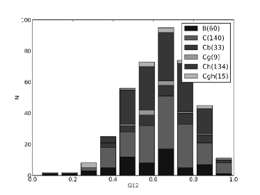
(a) C complex

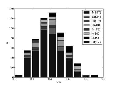
(b) S complex

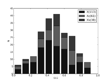
(c) X complex

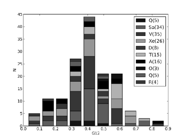
(d) Other complexes

Figure 1: Distributions of $G_{12}$ in asteroid taxonomic complexes. The different taxonomic classes are stacked from bottom to top in the histograms in the order listed in the legend.

Table 1: Means and standard deviations of $G_{12}$ for asteroid taxonomic complexes.

Complex	Nr of objects	mean	std
A	16	0.39	0.19
C	391	0.64	0.16
D	23	0.47	0.14
E	26	0.39	0.16
O	3	0.57	0.05
Q	72	0.41	0.14
R	4	0.24	0.18
S	584	0.41	0.16
V	35	0.41	0.14
X	212	0.48	0.19

Based on the approximated $G_{12}$ distributions for the different taxonomic complexes (Table 1), we can compute the probability for an asteroid to belong to a given taxonomic complex as the a posteriori probability using Bayes’s rule. For example, the probability for an asteroid to belong to the C complex can be computed using

$$p_{C}(x\in C\mid G_{12})=A\,pr(x\in C)\,p(G_{12}\mid x\in C),$$ (4)

where $A$ is a normalization constant, $p_{C}(x\in C\mid G_{12})$ is the a posteriori probability for an asteroid $x$ to belong to the C complex, given a particular $G_{12}$ value; $pr(x\in C)$ is the a priori probability for an asteroid $x$ to belong to the C complex; and $p(G_{12}\mid x\in C)$ is the probability for an asteroid $x$ to have a specific $G_{12}$ value, given that it belongs to the C complex.

As estimates for the probabilities $p(G_{12}\mid x\in C)$, we adopt the Gaussian approximations for the empirical $G_{12}$ distributions of different taxonomic complexes. We make use of three different a priori distributions: (1) a uniform a priori distribution; (2) an a priori distribution based on the frequency of C, S, and X complex objects among asteroids with taxonomy defined in the Planetary Data System database (PDS, see Neese, 2010); (3) an a priori distribution based on the frequencies of C, S, and, X complexes in different parts of the main asteroid belt (inner, mid, and outer main belt) from the PDS database. Testing the results obtained with different a priori distributions is important for insuring that the results are driven by data and not by the a priori distribution.

The probabilities computed based on the different a priori distributions should agree for different a priori assumptions if the photometric parameter brings substantial information overriding the information contained in the different a priori distributions. By using choice (1), we assume no previous knowledge of asteroid taxonomy. By using choice (2), we assume that the a priori probability for an asteroid $x$ to belong to a specific complex is equal to the frequency of occurrence of asteroids of that complex in the sample of known asteroid taxonomies in the PDS database. This means that, for the C, S, and X complexes, we use the a priori probabilities equal to $0.33$, $0.49$, and $0.18$, respectively. To derive the a priori distribution for choice (3), we first divide the main asteroid belt into three regions: the inner (region I), mid (region II), and outer main belt (region III). The boundaries between the regions are based on the most prominent Kirkwood gaps. Region I lies between the 4:1 resonance ($2.06$ AU) and 3:1 resonance ($2.5$ AU). Region II continues from the end of region I out to the 5:2 resonance ($2.82$ AU). Region III extends from the outer edge of region II to the 2:1 resonance ($3.28$ AU). The frequencies derived for those regions are as follows: for the C complex, 0.19 (I), 0.38 (II), 0.45 (III); for the S complex, 0.70 (I), 0.42 (II), 0.33 (III); and, for the X complex, 0.11 (I), 0.20 (II), 0.22 (III). The regional frequencies are also computed based on the data available in the PDS database. In general, a better choice of the a priori distributions would be based on debiased ratios of taxonomic complexes, but those are not available. In general, a single asteroid can have non-zero probability for belonging to two or more complexes.

The probability for an asteroid family being dominated, for example, by the C complex can be computed as

$$P_{C}=\frac{\sum_{i=1}^{N_{mem}}p^{(i)}_{C}}{N_{C}+N_{S}+N_{X}},$$ (5)

where $N_{C}$, $N_{S}$, and $N_{X}$ are the numbers of asteroids classified as belonging to the C, S, and X complexes, $N_{mem}$ is the number of members in a family, and $p^{(i)}_{C}$ is the probability of member $i$ belonging to the C complex. The probabilities for an asteroid family being dominated by other complexes can be computed in a similar fashion. In practice, $P_{C}$ represents the probability that a random asteroid from a given family would be of C complex.

2.3 Validation

In order to validate the method described in Sec. 2.2, we have checked the number of correct taxonomic complex classifications of asteroids with known taxa via so-called N-folded tests. First, we derived the frequencies of different taxonomic complexes, skipping 50 random asteroids in each complex which we later use for testing. The general frequencies for the C, S, and X complexes were $0.33$, $0.52$, and $0.15$. In the inner, mid, and outer main belt, the numbers are, respectively, as follows: 0.20, 0.72, and 0.09; 0.37, 0.44, and 0.18; 0.46, 0.37 and 0.17. Those frequencies are then used as priors in Eq. 4.

The success ratio is measured as

$$R_{s}=\frac{N_{corr}}{N_{total}},$$ (6)

where $N_{corr}$ is the number of correct identifications among $N_{total}$ asteroids.

Using the uniform a priori distribution (1) results in a $64\%$ overall success ratio ($80\%$ for the C complex, $60\%$ for the S complex, and $52\%$ for the X complex). Using the overall frequencies (2) results in a $63\%$ overall success ratio ($98\%$ for the C complex, $68\%$ for the S complex and $22\%$ for the X complex). The last choice (3) leads to a $63\%$ overall success ratio ($96\%$ for the C complex, $72\%$ for the S complex and $22\%$ for the X complex). We compared these success ratios with those arising from random guessing. We conclude that there is general improvement in success ratios for all the taxonomic complexes.

3 Results and discussion

We explore the correlation of the photometric parameter $G_{12}$ with the taxonomic classification based on about half a million asteroid phase curves in the Lowell Observatory database (Oszkiewicz et al., 2011). In Fig. 2, we present the distribution of the orbital proper elements color-coded with the $G_{12}$ values, with with a larger number of asteroids included as compared to the results in Oszkiewicz et al. (2011). The updated figure strengthens our previous findings of $G_{12}$ homogeneity within asteroid families. Even though the distributions of the $G_{12}$ values in asteroid families can be broad, asteroids in families stand out and tend to have similar values of $G_{12}$ (Oszkiewicz et al., 2011). Asteroids having disparate $G_{12}$ values but still identified as family members can be so-called interlopers, asteroids originating from a differentiated parent body, and asteroids with differently evolved surfaces. This result is consistent with previous findings on the homogeneity of asteroid families. For example, it was previously found that asteroids within families can share similar spectral properties (Cellino et al., 2002) and colors (Ivežić et al., 2002). The tendency toward family homogeneity might be helpful in deriving the family membership. Note that this tendency does not support the claim that asteroid families originate from differentiated parent bodies, since objects resulting from the disruption of a differentiated parent body would show differing photometric phase curves. Therefore, the distribution of the $G_{12}$ values could contribute to the understanding the origin and evolution of asteroid families. $G_{12}$ could also be used, along with the proper elements, for asteroid family classification. The trend from smaller average $G_{12}$ values for the inner belt to larger $G_{12}$ values for the outer belt is consistent with the distribution of C and S class asteroids in the asteroid belt. We also note that the $G_{12}$ values of family members in Fig. 2 correlate well with the SDSS color-color plot (Ivežić et al., 2002). The correlation relates to the fact that both the SDSS colors and $G_{12}$ correlate with asteroid taxonomy.

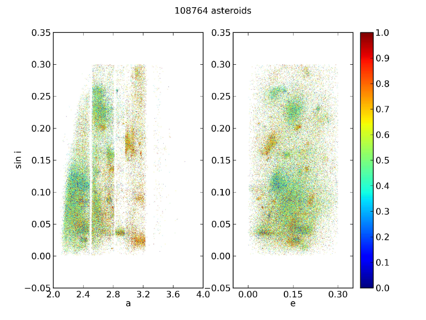
Figure 2: Distribution of asteroid proper elements, color-coded according to the $G_{12}$ value.

In Fig. 3, we plot the distribution of asteroids in SDSS color-color space, coded according to the $G_{12}$ value. The $x$-axis is defined as $a^{*}=0.89(g-r)+0.45(r-i)-0.57$ and $y$-axis as $i\!-\!z$, where $g$, $r$, $i$, and $z$ are magnitudes in the SDSS filters. The two clouds correspond to the C and S class asteroids, and the V class asteroids are located in the lower right corner of the plot (with large $a^{*}$ and small $i\!-\!z$ values). C class asteroids tend to have, on average, larger values of $G_{12}$, S class smaller, and V class often very small $G_{12}$ values.

Figure 3: Distribution of asteroids in $(a^{*},i\!-\!z)$ SDSS color space, color-coded according to the $G_{12}$ value.

To investigate the correlation of $G_{12}$ with taxonomy, we further extracted taxonomic classifications from PDS. The data set contains entries for 2615 objects. Each of the eight taxonomies represented produced classifications for a subset of the objects: Tholen (1984, 1989) – 978 objects; Barucci et al. (1987) – 438 objects; Tedesco (1989), Tedesco et al. (1989) – 357 objects; Howell et al. (1994) – 112 objects; Xu et al. (1995) – 221 objects; Bus and Binzel (2002) – 1447 objects; Lazzaro et al. (2004) – 820 objects; and DeMeo et al. (2009) – 371 objects. We make use of the Bus and Binzel classification, which contains the largest number of asteroids. We divide our sample into thirteen complexes: A, C [B, C, Cb, Cg, Ch, Cgh], D [D, T], E [E, Xe], M, P, O, Q [Q, Sq], R, S [S, Sa, Sk, Sl, Sr, K, L, Ld], V, X [X, Xc, Xk], and U. We produce histograms of the $G_{12}$ values for each of them (see Fig. 1). Each taxonomic complex is then approximated by a Gaussian distribution. The means and standard deviations of the $G_{12}$ values for all the complexes are listed in Table 1. Most of the complexes contain too few objects for meaningful statistical treatment, except for the S, C, and X complexes. The means of the distributions for the S, C, and X complexes are clearly different.

The S complex has a mean $G_{12}$ of $0.41$, the C complex has a higher mean $G_{12}$ of $0.64$, and the X complex is intermediate having a mean of $0.48$. In general, asteroids within the same taxonomic complex could have varying surface properties (for example, different regolith porosities or grain-size distributions) leading to different $G_{12}$ values, resulting in broad $G_{12}$ histograms for a complex. An additional challenge follows from the fact that the $G_{12}$ distributions for the different taxonomic complexes partially overlap. Based on those distributions, selected priors (see Sec. 2.2) and previously obtained photometric parameters (Oszkiewicz et al., 2011) for each of the half a million asteroids, we computed the C, S, and X complex classification probabilities for each asteroid. Due to broad and overlapping $G_{12}$ distributions, these probabilities are often be similar enough to prevent a meaningful classification of the asteroid into any one of the complexes.

For some asteroids, $G_{12}$ can, however, be a good indicator of taxonomic complex. For example, an asteroid with $G_{12}=0.8$ from the outer belt has a probability of 82% for being of C complex and low probabilities of being of S or X complex (5% and 13%). If we assume no knowledge on asteroid location nor on the frequency of different taxonomic complexes (uniform prior (1)), an asteroid with $G_{12}=0.8$ would still have a chance of 70% for being of C complex. For reference, we list the probabilities for an asteroid with $G_{12}=0.8$ being of C, S, and X complex in Table 2, assuming different priors and different locations in the belt (or no knowledge on location in the belt).

Table 2: Example result for a single asteroid. Probabilities for an asteroid with $G_{12}=0.8$ to be of C, S, and X complex.

Prior	$P_{c}$	$P_{s}$	$P_{x}$
(1)	70%	6%	24%
(2)	76%	10%	14%
(3) Inner MB	66%	21%	13%
(3) Mid MB	79%	7%	14%
(3) Outer MB	82%	5%	13%

Asteroid families containing, for example, a large number of asteroids with high $G_{12}$ values resulting in high $P_{c}$ values could be identified as C-complex preponderant. As a prime example, we indicate the Dora family having the mean $G_{12}=0.7$ and standard deviation $\sigma_{G_{12}}=0.18$, which result in a high C-complex preponderance probability. The $G_{12}$ distribution (Fig. LABEL:family) for the Dora family also matches nicely the C-complex distribution profile.

Table 3: The number of family members included in the study, the mean and standard deviation of $G_{12}$, and the probabilities of C, S, and X complex preponderance based on the a priori distributions (1), (2), and (3) (see above). Family classifications are from Nesvorny (2010).

	General			(1) Uniform			(2) Frequency			(3) Location
	$G_{12}$ statistics			prior			prior			prior
Family or	Nr of	$G_{12}$	$G_{12}$	$P_{C}$	$P_{S}$	$P_{X}$	$P_{C}$	$P_{S}$	$P_{X}$	$P_{C}$	$P_{S}$	$P_{X}$
cluster	mem.	mean	std.
Adeona	987	0.64	0.2	0.49	0.21	0.29	0.55	0.27	0.18	0.55	0.27	0.18
Aeolia	55	0.66	0.23	0.51	0.2	0.29	0.54	0.29	0.16	0.57	0.25	0.17
Agnia	472	0.58	0.21	0.42	0.27	0.31	0.47	0.34	0.19	0.47	0.34	0.19
Astrid	94	0.64	0.23	0.49	0.22	0.29	0.43	0.45	0.12	0.55	0.27	0.17
Baptistina	1966	0.53	0.18	0.36	0.31	0.33	0.46	0.32	0.22	0.26	0.62	0.12
Beagle	38	0.64	0.23	0.5	0.21	0.29	0.6	0.21	0.18	0.6	0.21	0.18
Brangäne	37	0.68	0.19	0.53	0.19	0.28	0.64	0.19	0.18	0.6	0.24	0.17
Brasilia	186	0.49	0.21	0.31	0.35	0.34	0.4	0.37	0.23	0.4	0.37	0.23
Charis	136	0.61	0.21	0.45	0.25	0.31	0.55	0.25	0.2	0.55	0.25	0.2
Chloris	200	0.63	0.17	0.48	0.22	0.3	0.59	0.22	0.19	0.55	0.28	0.18
Clarissa	41	0.64	0.22	0.49	0.22	0.29	0.42	0.46	0.12	0.42	0.46	0.12
Datura	4	0.41	0.2	0.23	0.42	0.35	0.3	0.45	0.25	0.17	0.72	0.11
Dora	528	0.7	0.18	0.56	0.16	0.28	0.67	0.16	0.17	0.63	0.2	0.16
Emma	111	0.66	0.23	0.52	0.19	0.29	0.59	0.24	0.17	0.63	0.19	0.18
Emilkowalski	2	0.56	0.07	0.39	0.28	0.33	0.45	0.35	0.2	0.45	0.35	0.2
Eos	3413	0.64	0.19	0.5	0.21	0.29	0.56	0.27	0.18	0.6	0.21	0.19
Erigone	806	0.63	0.19	0.48	0.22	0.3	0.54	0.28	0.18	0.4	0.48	0.12
Eunomia	4707	0.51	0.18	0.33	0.34	0.33	0.37	0.42	0.2	0.37	0.42	0.2
Flora	6316	0.53	0.18	0.35	0.32	0.33	0.26	0.63	0.11	0.26	0.63	0.11
Gefion	1938	0.56	0.19	0.39	0.29	0.32	0.49	0.3	0.21	0.44	0.36	0.19
Hestia	103	0.55	0.2	0.39	0.29	0.32	0.44	0.37	0.19	0.44	0.37	0.19
Hoffmeister	341	0.68	0.22	0.53	0.19	0.28	0.63	0.19	0.18	0.59	0.24	0.17
Hygiea	1729	0.66	0.21	0.51	0.2	0.29	0.61	0.2	0.18	0.61	0.2	0.18
Iannini	30	0.45	0.23	0.26	0.4	0.34	0.29	0.5	0.21	0.29	0.5	0.21
Juno	359	0.52	0.21	0.36	0.32	0.33	0.27	0.61	0.11	0.4	0.4	0.2
Karin	159	0.54	0.22	0.38	0.3	0.32	0.29	0.59	0.12	0.47	0.31	0.22
Kazvia	12	0.6	0.21	0.45	0.24	0.31	0.51	0.31	0.18	0.51	0.31	0.18
Konig	58	0.68	0.17	0.53	0.18	0.28	0.6	0.23	0.17	0.6	0.23	0.17
Koronis	2913	0.58	0.2	0.42	0.27	0.31	0.52	0.28	0.21	0.52	0.28	0.21
Lau	6	0.54	0.17	0.39	0.28	0.33	0.5	0.28	0.21	0.5	0.28	0.21
Lixiaohua	171	0.64	0.23	0.5	0.21	0.29	0.43	0.45	0.12	0.59	0.22	0.19
Lucienne	37	0.5	0.21	0.33	0.34	0.33	0.25	0.64	0.11	0.25	0.64	0.11
Maria	2009	0.5	0.2	0.33	0.34	0.33	0.37	0.42	0.2	0.37	0.42	0.2
Massalia	1911	0.56	0.2	0.39	0.29	0.32	0.44	0.37	0.19	0.3	0.58	0.12
Meliboea	40	0.68	0.14	0.55	0.17	0.28	0.62	0.21	0.17	0.67	0.16	0.17
Merxia	425	0.53	0.22	0.36	0.31	0.33	0.46	0.33	0.22	0.41	0.39	0.2
Misa	220	0.68	0.21	0.54	0.18	0.28	0.6	0.23	0.17	0.6	0.23	0.17
Naema	98	0.66	0.2	0.51	0.2	0.29	0.58	0.25	0.17	0.62	0.2	0.18
Nemesis	258	0.68	0.19	0.54	0.18	0.28	0.64	0.18	0.18	0.6	0.23	0.17
Nysa-Polana	8289	0.57	0.19	0.4	0.28	0.32	0.46	0.35	0.19	0.31	0.57	0.12
Padua	372	0.66	0.2	0.52	0.19	0.29	0.59	0.24	0.17	0.59	0.24	0.17
Rafita	477	0.55	0.2	0.39	0.29	0.32	0.48	0.3	0.21	0.44	0.37	0.19
Sulamitis	92	0.66	0.21	0.52	0.2	0.29	0.62	0.2	0.18	0.45	0.43	0.12
Sylvia	30	0.56	0.26	0.43	0.25	0.31	0.53	0.27	0.21	0.46	0.37	0.17
Telramund	240	0.58	0.23	0.42	0.27	0.31	0.47	0.34	0.19	0.51	0.28	0.21
Terentia	7	0.41	0.2	0.24	0.4	0.36	0.15	0.74	0.11	0.32	0.42	0.25
Themis	2559	0.69	0.19	0.55	0.17	0.28	0.62	0.22	0.17	0.66	0.17	0.17
Theobalda	60	0.61	0.22	0.47	0.23	0.3	0.39	0.49	0.12	0.57	0.24	0.19
Tirela	818	0.61	0.2	0.46	0.24	0.3	0.56	0.24	0.2	0.56	0.24	0.2
Veritas	291	0.68	0.21	0.54	0.18	0.28	0.61	0.22	0.17	0.65	0.18	0.17
Vesta	8445	0.5	0.18	0.32	0.35	0.34	0.36	0.44	0.2	0.22	0.66	0.11
18405	24	0.63	0.16	0.48	0.22	0.3	0.51	0.32	0.17	0.6	0.21	0.19
18466	94	0.49	0.22	0.31	0.35	0.34	0.24	0.65	0.11	0.36	0.44	0.2

In order to check how well we can identify asteroid families as being dominated by one of the taxonomic complexes, we produce $G_{12}$ histograms for the different asteroid families (histograms for chosen families are presented in Fig. LABEL:family, histograms for the remaining families can be found in supplementary materials; numerical values are in Table LABEL:mean) and use methods based on Bayesian statistics (described in Sec. 2) to establish the dominant taxonomic complex. We then compare our results with the published results from other studies.

Table 4: The normalized $G_{12}$ distributions for asteroid families as listed in Table LABEL:mean. The family classification is from PDS (Nesvorny, 2010). The dashed line indicates the distribution weighted with one over the sum of the absolute two-sided errors, and the solid line is the unweighted histogram. For comparison, we plot the a posteriori functions for the different taxonomic complexes (the C complex is indicated by the thick dashed line, the S complex by the thick dotted line, and the X complex by the thick dash-dotted line) based on prior (2).

Deciding on the taxonomic complex preponderance based on $G_{12}$ can prove difficult and one should be careful in drawing conclusions when the resulting probabilities for the different complexes are similar. To pick asteroid families that show a preference in taxonomic complex, we set the following requirements:

1. The minimum number of asteroids in the sample must be around 100 or more.

2. The probability for preponderance must be the highest for all the assumed a priori probabilities. This is to make sure that the inference is driven by data and not by the a priori distribution.

3. The probability for the preponderant complex must be close to 50% or more for all the assumed a priori distributions.

Table LABEL:mean lists the probabilities for taxonomic complex preponderance, along with the family means and standard deviations of the $G_{12}$ values. Several families have too few members to draw any conclusions. Some of the families result in very similar taxonomic complex preponderance probabilies for each complex and therefore no complex can be indicated as dominating. For some families the computed probabilities suggest different preponderant complex based on different a priori probabilies. For those families no conclusions could be made. Several families, however show clear preference of taxonomic complex. Those include:

• (145) Adeona (region II): The $G_{12}$ distribution for the Adeona family contains 987 asteroids and is visibly shifted towards high $G_{12}$ values. Based on the computed probabilities, the Adeona family seems to be dominated by C complex objects: the C complex probabilities for the family are 49%, 55%, and 55% based on the a priori distributions (1), (2), and (3), respectively, which agrees with the literature. The computed C complex preponderance probabilities are 20% to 37% higher than those for the other complexes. Visual inspection of the histogram also suggests that the majority of asteroids in this family must have come from the C-complex distribution (see Fig. LABEL:family). The $G_{12}$ distribution for this family is smooth. In the literature, the Adeona family has 12 members with known spectroscopic classification: 9 in class Ch, 1 in C, 1 in X, 1 in D, and 1 in class Xk (Mothé-Diniz et al., 2005).

• (627) Charis (region III): The Charis cluster seems to be strongly C complex preponderant. C complex preponderance probabilities are 45%, 55% and 55% for the a priori distributions (1), (2), and (3). The $G_{12}$ distribution is smooth and clearly shifted towards large $G_{12}$ values. The profile of the $G_{12}$ distribution also matches the $G_{12}$ distribution profile of the C complex.

• (410) Chloris (region II): The profile of the $G_{12}$ distribution for the Chloris cluster is similar to that of the Charis family, also matching the profile of the $G_{12}$ distribution for the C complex. The computed probabilities also indicate C complex preponderance: they are 48%, 59%, and 55% for the a priori distributions (1), (2), and (3), and are about 20% larger than for any other complex. This cluster has also been spectroscopically characterized as C complex dominant by Bus (1999).

• (668) Dora (region II): The Dora family is strongly C complex dominated. The probabilities of C complex preponderance are 56%, 67%, and 63% for the priori distributions (1), (2), and (3), and are 28–51% higher than those for the S and X complexes. Also, the $G_{12}$ distribution is smooth and matches better the C complex distribution than the S or X complex distributions. In the literature, Dora has 29 members with known spectra, all belonging to the C complex (24 in class Ch, 4 in C, and 1 in class B) (Mothé-Diniz et al., 2005; Bus, 1999).

• (283) Emma (region III): The $G_{12}$ distribution for the Emma family is smooth and dominated by asteroids with large $G_{12}$ values. The probability of Emma being C complex preponderant is 52%, 59%, and 63% for the a priori distributions (1), (2), and (3). These probabilities are about 30% larger than those for the S and X complexes. Therefore, Emma can be classified as C complex preponderant.

• (1726) Hoffmeister (region II): The Hoffmeister family is C complex dominant. The C complex preponderance probability is 53%, 63%, and 59% for the a priori distributions (1), (2), and (3), and is about 25% larger than those of the S or X complex preponderance. There are 10 members of this family with known spectra: 8 in class C (4 in class C, 3 in Cb, and 1 in class B), 1 in Xc, and 1 in class Sa (Mothé-Diniz et al., 2005). The $G_{12}$ distribution for the Hoffmeister family is peculiar and steadily increasing towards larger $G_{12}$ values.

• (10) Hygiea (region III): Similarly to the Hoffmeister family, the Hygiea family is C complex preponderant. The C complex preponderance probabilities are 51%, 61%, and 61% for the a priori distributions (1), (2), and (3). The probabilities for the other complexes are about 20–40% smaller. Most of the asteroids in the family are of class B (C complex) (Mothé-Diniz et al., 2005).

• (569) Misa (region II): The Misa family is C complex preponderant. The C complex preponderance probabilities are 54%, 60%, and 60% for the a priori distributions (1), (2), and (3), and are about 35% higher than those of being S or X complex preponderant.

• (845) Naema (region III): The Naema family is C complex preponderant. The C complex preponderance probabilities are 51%, 58%, and 62% for the a priori distributions (1), (2), and (3), and are about 20–40% higher than those of being S or X complex preponderant.

• (128) Nemesis (region II): The Nemesis family is C complex preponderant. The C complex preponderance probabilities are 54%, 64%, and 60% for the a priori distributions (1), (2), and (3), and are about 25–35% higher than those of being S or X complex preponderant.

• (363) Padua (region II): The $G_{12}$ distribution for the Padua family is shifted towards large values of $G_{12}$ and indicates C complex preponderance. The C complex preponderance probabilities are 52%, 59%, and 59% for the a priori distributions (1), (2), and (3). The Padua family has 9 members with spectral classification. Most of them are X class asteroids (6 in class X and 1 in Xc), and there are also 2 C class members (Bus, 1999; Mothé-Diniz et al., 2005).

• (24) Themis (region III): The Themis family is C complex preponderant which agrees with the literature analyses. The C complex preponderance probabilities are 55%, 62%, and 66% for the a priori distributions (1), (2), and (3), and are about 30–50% larger than those of being S or X complex preponderant. In the literature, 43 Themis family asteroids have spectra available. The taxonomy of these asteroids is homogeneous: there are 36 asteroids from the C complex (6 in class C, 17 in B, 5 in Ch, and 8 in class Cb) and 7 asteroids from the X complex (5 in class X, 1 in Xc, and 1 in Xk) (Mothé-Diniz et al., 2005; Florczak et al., 1999).

• (490) Veritas (region III): The Veritas family is C complex preponderant which agrees with the literature analyses. The C complex preponderance probabilities are 54%, 61%, and 65% for the a priori distributions (1), (2), and (3), and are about 25–50% higher than those of being S or X complex preponderant. In the literature, the Veritas family has 8 members with known spectra, all of them belonging to the C complex: 6 in class Ch, 1 in C, and 1 in class Cg (Mothé-Diniz et al., 2005).

For a number of families it was not possible to indicate preponderant taxonomic complex. Out of those a particular case is the Nysa-Polana family, which shows a clear differentiation into two separate regions.

(44) Nysa - (142) Polana (region I): The taxonomic preponderance probabilities for the Nysa-Polana family are similar for all the complexes, therefore no single complex can be indicated as preponderant. Additionally, the different a priori distributions result in differing preponderances. It has been previously suggested (Cellino et al., 2001) on the basis of spectral analysis that the Nysa-Polana family is actually composed of two distinct families, which is incompatible with the hypothesis of common origin. The first one (Polana) was suggested to be composed of dark objects and the second one (Mildred) of brighter S class asteroids. Parker et al. (2008) has performed a statistical analysis and showed that, based on the SDSS colors, it is possible to separate the Nysa-Polana region into two families. in order to assess this suggestion, we plot the distribution of proper elements (semimajor axis and eccentricity) of the asteroids from the Nysa-Polana region in Fig. 4, color coded according to the $G_{12}$ values and the SDSS $a^{*}$ values for comparison.

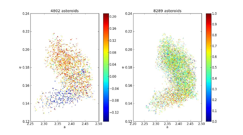
Figure 4: Distribution of proper elements for asteroids in the Nysa-Polana region, color coded according to the SDSS $a^{*}$ values (left) and the $G_{12}$ values (right). The sizes of the points correspond to the errors in $G_{12}$ and SDSS $a^{*}$.

The two taxonomically different regions stand out both in $G_{12}$ and in SDSS $a^{*}$. The sample size for the plot color-coded according to the $G_{12}$ value is much larger than that color-coded with the SDSS $a^{*}$ value. The $G_{12}$ plot suggests that there is much more structure in the Nysa-Polana region and that there might be more than the two main taxonomic groups present, or that they might be more mixed. In their spectral analyses, Cellino et al. (2001) also found three asteroids of class X, next to the 11 Tholen F class and 8 S class asteroids. For reference, we list the $G_{12}$ values for the main members of the Nysa-Polana region in Table 5. Generally, it might turn out difficult to separate the two groups as they seem quite strongly intermixed. We carried out a $k$-means clustering operation for this region (with $k=2$). Clustering in the proper elements and in the SDSS $a^{*}$ parameter gave, overall, the same results as using the proper elements and the $G_{12}$ parameter.

Table 5: The $G_{12}$ parameters for the main members of Nysa-Polana family.

Designation	H[mag]	$G_{12}$	taxon
44 Nysa	$+6.9^{+0.05}_{-0.05}$	$+0.08^{+0.07}_{-0.07}$	Xe (Neese, 2010)
142 Polana	$+10.20^{+0.013}_{-0.014}$	$+0.69^{+0.09}_{-0.09}$	B (Neese, 2010)
135 Hertha	$+8.13^{+0.01}_{+0.01}$	$+0.32^{+0.08}_{-0.08}$	Xk (Neese, 2010)
878 Mildred	$+14.51^{+0.03}_{-0.03}$	$+0.79^{+0.17}_{-0.17}$

Other families for which no conclusion could be made, but the shape of the $G_{12}$ distributions can still be discussed are:

• (847) Agnia (region II, also called (125) Liberatrix): altogether 472 members are considered for the Agnia family, with a smooth but wide $G_{12}$ distribution. The diverse $G_{12}$ values basically span through the entire range of possible $G_{12}$ values. The decision requirement (3) is not met for this family and therefore no definite conclusions can be made. However, based on the large $G_{12}$ values for many members of the family, we would suggest that the Agnia family can contain large numbers of both S and C complex asteroids. In the literature, the Agnia family has 15 members with known spectroscopic taxonomy, all belonging to the S complex (8 in class Sq, 6 in S, and 1 in Sr) (Mothé-Diniz et al., 2005; Bus, 1999).

• (1128) Astrid (region II): The $G_{12}$ values for 94 members of the Astrid family result in a high probability of C complex preponderance for the a priori distributions (1) and (3) and almost equal probability of C and S complex preponderance for the a priori distribution (2). Accordingly, no conclusions can be made. In the literature, the Astrid family has 5 spectrally characterized members, all of which belong to the C complex (4 class C, 1 in Ch) (Mothé-Diniz et al., 2005; Bus, 1999).

• (298) Baptistina (region I): The $G_{12}$ distribution for the Baptistina family is quite broad and results in similar probabilities for all the complexes for the a priori distributions (1) and (2). For the a priori distribution (3), the probability of S complex preponderance is the largest. In the literature, the Baptistina family has 8 spectrally characterized members. These asteroids tend to have different spectral classifications: 1 in class Xc, 1 in X, 1 in C, 1 in L, 2 in S, 1 in V, and 1 in class A (Mothé-Diniz et al., 2005). Due to the lack of fulfillment of the requirements (2) and (3), we cannot evaluate the taxonomic preponderance in this family.

• (293) Brasilia (region III): The $G_{12}$ distribution of the Brasilia family is wide (spreading through the entire range of possible $G_{12}$ values). The resulting preponderance probabilities are similar for all the taxonomic complexes. In the literature, 4 members of the Brasilia family have known spectroscopic classification: 2 in class X, 1 in C, and 1 in class Ch (Mothé-Diniz et al., 2005).

• (221) Eos (region III): The Eos family has 92 members that have taxonomic classification. There are 26 members in class T, 17 in D, 12 in K, 8 in Ld, 13 in Xk, 4 in Xc, 5 in X, 3 in L, 2 in S, 1 in C, and 1 class B. The family has an inhomogeneous taxonomy (Mothé-Diniz et al., 2005). This means that 43 asteroids originate from D complex, 25 from the S complex, 22 from the X complex, and 2 from the C complex. In our treatment, we have decided to refrain from considering complexes other than the three main ones, so indicating D complex preponderance is not possible. The $G_{12}$ histogram for Eos is shifted towards intermediate and large $G_{12}$ values, and is more indicative of C complex rather than S or X complex preponderance.

• (163) Erigone (region I): The $G_{12}$ distribution for this family is slightly shifted tpwards large $G_{12}$s. Erigone has 48% and 54% probabilities of C complex preponderance based on the a priori distributions (1) and (2), and a 48% probability of S complex preponderance based on the a priori distribution (3). Therefore, no particular complex can be indicated as preponderant.

• (15) Eunomia (region II): The Eunomia family has a smooth $G_{12}$ distribution with a profile matching the combined profile of all complexes. The probabilities of Eunomia being S complex preponderant are 34%, 42%, and 42% for the a priori distributions (1), (2), and (3) and are the largest among the different complexes, which agrees with the literature analyses. The difference between the S and the other complex preponderance probabilities are however only about 10%. Generally, the probabilities are below the required 50%, so no complex can be indicated as preponderant. In the literature, the Eunomia family has 43 members that have observed spectra, most members classified as belonging to the S complex. There are 16 members in class S (including (15) Eunomia), 2 in Sk, 10 in Sl, 1 in Sq, 7 in L, 4 in K, 1 in Cb, 1 in T, and 1 in class X (Lazzaro et al., 1999; Mothé-Diniz et al., 2005).

• (8) Flora (region I): The $G_{12}$ distribution for the Flora family is smooth with a mean at $G_{12}=0.53$. The probability of Flora being S complex dominant is the largest and is 63% for the a priori distributions (2) and (3). Assuming a uniform a priori distribution leads to almost equal taxonomic complex preponderance probabilities. In the literature, Flora is considered S complex preponderant (Florczak et al., 1998). However, due to the lack of fulfillment of the decision requirements, we do not make a final conclusion on the taxonomic preponderance in this family.

• (1272) Gefion (region II, also identified as (1) Ceres or (93) Minerva): In the literature, the Gefion family has 35 members that have spectral classification. Out of these asteroids, 31 belong to the S complex (26 in class S, 2 in Sl, 2 in Sr, 1 in Sq, and 1 in L), 2 belong to the C complex (1 in class Cb class and 1 in Ch), and there is 1 X class asteroid (Mothé-Diniz et al., 2005). Our complex preponderance probability computation results in similar probabilities for all three complexes and is inconclusive for this family. The $G_{12}$ distribution for Gefion spreads through all the complexes and is slightly shifted towards higher $G_{12}$ values.

• (46) Hestia (region II): The $G_{12}$ distribution for the Hestia family is similar to that of the Gefion family. Thus, no conclusions can be made as the probabilities of taxonomic preponderance are comparable for all the complexes.

• (3) Juno (region II): In the case of the Juno family, the $G_{12}$ distribution is similar to the two previous families, the taxonomic complex preponderance probabilities are similar for all the complexes. Therefore, no single complex can be indicated as preponderant.

• (832) Karin (region III): For the Karin family, the preponderance probabilities are similar for all the complexes for the a priori distribution (1). Therefore, no single complex can be indicated as preponderant. For the a priori distributions (2) and (3), the probabilities are discordant. The $G_{1}2$ distribution for this family is wide, whithout a clear prefference for any of the complexes.

• (158) Koronis (region III): In the literature, the Koronis family has 31 members with spectral classification. There are 29 asteroids from the S complex (19 in class S, 1 in Sk, 3 in Sq, 2 in Sa, and 4 in class K), 1 from class X, and 1 from class D. The spectra of eight of these members have been analyzed by Binzel et al. who found a moderate spectral diversity among these objects (Binzel et al., 1993; Mothé-Diniz et al., 2005). In our computation, the Koronis family has the highest chance of being C complex dominated. However, the probability of being S dominant cannot be excluded as it is also quite high. Due to the lack of fulfillment of the decision requirement (3), we do not make a final conclusion on the taxonomic preponderance in this family.

• (3556) Lixiaohua (region III): The taxonomic preponderance probabilities for the Lixiaohua family are quite high for the C complex. The probability of C complex preponderance are 50%, 43% and 59% for priors (1), (2), (3) respectively. However for prior (2) the probability of this family being S complex dominated is 45%. Therefore, no single complex can be indicated as preponderant. $G_{12}$ distribution for this family spans though at the full range of allowed $G_{12}$ and shows surplus of high $G_{12}$s.

• (170) Maria (region II): Even though the Maria family has the largest probability of being S complex preponderant, which agrees with the literature, no conclusions should be made as the probabilities of the C and X complex preponderance are large . In the literature, the Maria family has 16 members which have spectral classification, all belonging to the S complex (4 in class S, 5 in L, 4 in Sl, 2 in K, and 1 class Sk) (Mothé-Diniz et al., 2005). $G_{12}$ distrubution for this family matches the combine $G_{12}$ profile from all the complexes.

• (20) Massalia (region I): The taxonomic preponderance probabilities for the Massalia family are similar for all the complexes. Therefore, no single complex can be indicated as preponderant. Additionally, the three different a priori distributions result in differing preponderant complexes. $G_{12}$ distribution for Massalia family seems to be slightly shifted towards high $G_{12}$s.

• (808) Merxia (region II): The taxonomic preponderance probabilities for the Merxia family are inconclusive as none of the computed probabilities arises significantly above the rest. In the literature, the Merxia family has 8 asteroids spectrally characterized: 1 member belongs to the X complex while the remaining 7 members belong to the S complex (3 in class Sq, 2 in S, 1 in Sr, and 1 class Sl) (Mothé-Diniz et al., 2005; Bus, 1999). $G_{12}$ distribution for this family is wide and also matches the total $G_{12}$ distribution of all complexes combined.

• (1644) Rafita (region II): The taxonomic preponderance probabilities for the Rafita family are similar for all the complexes. Therefore, no single complex can be indicated as preponderant. $G_{12}$ distribution for this family is wide and matches the total $G_{12}$ distribution of all complexes combined.

• (752) Sulamitis (region I): The $G_{12}$ distribution for the Sulamitis family is shifted towards large values of $G_{12}$, indicating C complex predominance. The C complex preponderance probabilities based on the a priori distributions (1) and (2) are large (52 and 62%). But based on the a priori distribution (3), the preonderance probability is only 45% and, therefore, we draw no final conclusions.

• (9506) Telramund (region III): The taxonomic preponderance probabilities for the Telramund family are similar for all the complexes. Therefore, no single complex can be indicated as preponderant. $G_{12}$ distribution for Teramund shows slight surplus of high $G_{12}$s.

• (1400) Tirela (region III): Tirela family also seems to be C complex predominant with the $G_{12}$ distribution shifted towardslarge $G_{12}$ values. However, due to the lack of fulfillment of the decision criterion (3), we refrain from making a final judgment.

• (4) Vesta (region I): The Vesta family is dominated by the V complex asteroids. Here we are not considering V complex asteroids. $G_{12}$ distribution for this family is wide and also matches the total $G_{12}$ distribution of all complexes combined.

• (18466) (region II): The taxonomic preponderance probabilities for the family of asteroid (18466) are similar for all the complexes. Therefore, no single complex can be indicated as preponderant. $G_{12}$ distribution for this family is wide, matches the total $G_{12}$ distribution of all complexes combined and shows a slight surplus of low to inermediate $G_{12}$s.

Number of families have to few members in our sample to be analyzed. Those include: (396) Aeolia (region II, 55 members), (656) Beagle (region III, 38 members), (606) Brangäne (region II, 37 members), (302) Clarissa (region I, 41 members), (1270) Datura (region I, 4 members), (14627) Emilkowalski (region II, 2 members), (4652) Iannini (region II 30 members), (7353) Kazuya (region II, 12 members), (3815) König (region II, 58 members), (10811) Lau (region III, 6 members), (1892) Lucienne (region I, 37 members), (137) Meliboea (region III, 40 members), (87) Sylvia (region III, 30 members), (1189) Terentia (region III, 7 members), (778) Theobalda (region III, 60 members), (18405) (region III, 24 members). Even though conclusions for those could not be made, it is worth mentioning several of these families. The $G_{12}$ distribution for Datura and Iannini families are shifted towards small $G_{12}$ values and could be candidates for an S complex preponderant families. Asteroid (1270) Datura is spectraly identified as S class (Neese, 2010). The $G_{12}$ distribution for the Theobalda family seems to be shifted towards C complex asteroids making it a candidate for C complex dominated. Asteroid (778) Theobalda is classified as F type (Neese, 2010). C complex preponderance is also possible for Meliboea family, which also has been previously classified as C complex preponderant (Mothé-Diniz et al., 2005). The C complex preponderance probabilities are 55%, 62% and 67% for the a priori distributions (1), (2), and (3), and are about 25–40% larger than those of being S or X complex preponderant. (137) Meliboea is spectrally classified as C class asteroid (Neese, 2010).

Overall, the strict decision criteria requirements result in C complex preponderance in the Adeona, Charis, Chloris, Dora, Emma, Hoffmeister, Hygiea, Misa, Naema, Nemesis, Padua, Themis, and Veritas families. Out of these, Adeona, Chloris, Dora, Hoffmester, Hygiea, Themis, and Veritas have spectral classifications that indicate C complex preponderance. Padua has only 9 members spectrally classified (7 of X complex and 2 of C complex). The Charis, Emma, Misa, Naema, and Nemesis families are yet to be spectrally classified.

There are no families that we can indicate as S or X complex preponderant mainly because those two are more difficult to separate. Also, there are no families which would have the distribution clearly shifted towards small $G_{12}$ values and fullfil our strict decision criteria.

We have also computed taxonomic complex probability for all asteroids having proper elements. Figure 5(a) shows the distribution of C, S, and X complex asteroids in the main asteroid belt weighted with the probabilities of belonging to the C, S, and X complexes. Fig. 5(b) shows the weighted fraction of different taxonomic complexes in the main belt. The overall distribution agrees with the general view of more S complex asteroids in the inner main belt and C complex asteroids dominating in the outer main belt (see, e.g., Gradie and Tedesco, 1982; Zellner, 1979; Mothé-Diniz et al., 2003; Yoshida and Nakamura, 2007; Bus, 1999). On the basis of the computed C, S, and X complex probabilities for each asteroid, we modify the distributions of $G_{12}$ values for the C, S, and X complexes in Fig. 6. The gap at $G_{12}=0.2$ is related to the numerical function that is used to derive the $H,\!G_{12}$ phase function, which is nondifferentiable at $G_{12}=0.2$ (for more details, see Muinonen et al., 2010a). This causes many asteroids to end up at $G_{12}=0.2$ in least-squares fitting. To avoid the artificial peak at $G_{12}=0.2$, we remove all asteroids with $G_{12}$ exactly equal to $0.2$. However, from the dip at $G_{12}=0.2$, it is clear that some valid solutions were thereby removed. Should the $H,\!G_{12}$ phase function be revised, we recommend that the $G_{1}=G_{1}(G_{12})$, $G_{2}=G_{2}(G_{12})$ functions are made differentiable. Figure 6 shows the updated $G_{12}$ distributions for the different complexes before and after correction for the $G_{12}=0.2$ artifact.

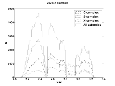
(a) Distribution of C, S, and X complex asteroids in the main belt.

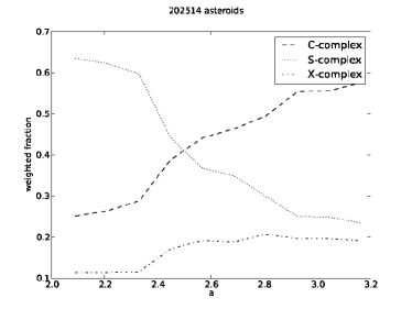
(b) Weighted fraction of asteroid complexes thought the main belt.

Figure 5: Composition of the main belt.

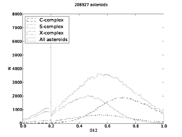
(a) With the artifact

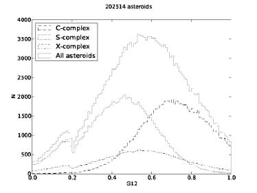
(b) Artifact corrected

Figure 6: Updated distribution of $G_{12}$ values in C, S and X complexes.

4 Conclusions

We have analyzed the photometric parameter $G_{12}$ for all known asteroids as well as $G_{12}$ distributions for asteroid families. We have strengthened our previous finding of $G_{12}$ homogeneity in some asteroid families and also confirmed a correlation between $G_{12}$ and taxonomy. $G_{12}$ could be potentially used in asteroid family membership classification. We have further analyzed asteroid families for C, S, or X complex preponderance.

We conclude that, although $G_{12}$ is related to surface properties, on its own it is mostly insufficient to unambiguously assign taxonomic complex of individual asteroids. Generally, the complex separation in the $G_{12}$ space is small. The $G_{12}$ distributions also overlap and, generally, no definitive conclusions should be made for individual objects based only on $G_{12}$ values. Rather probabilities of belonging to a given complex can be computed. All classification results for individual objects based on the $G_{12}$ values should be taken with caution and used rather to confirm previous results than to derive classifications based only on the current $G_{12}$ values.

In some cases $G_{12}$ values can, however, be an indication of asteroid taxonomic complex. Particularly, the C complex is the easiest to be separated, which was also confirmed by the high success ratio in the testing. Accordingly $G_{12}$ distributions can be used in verifying taxonomic complex preponderance in some asteroid families. We found a preponderance of C complex asteroids in several families. We compared our findings to the results available in the literature, and concluded that, based on the $G_{12}$ distributions in the families, we could confirm complex preponderance for several families available.

The $G_{12}$ values in conjunction with the SDSS colors could possibly result in a better separation of the different taxonomic complexes. An increased number of taxonomy classified asteroids and better quality data potentially leading to better constrained $G_{12}$ values could improve our knowledge of the $G_{12}$-taxonomy correlation. More detailed knowledge of asteroids surface properties would also benefit the classification problem. The Gaussian approximations of complex distributions could be replaced by more sophisticated distributions, and the a priori distributions for the Bayesian analysis could be replaced by those deriving from debiased taxonomic distributions. Particularly, a continuous debiased function describing the fraction of different complexes throughout the belt could be used.

References

- Barucci et al. (1987) Barucci, M. A., Capria, M. T., Coradini, A., Fulchignoni, M., 1987. Classification of asteroids using G-mode analysis. Icarus 72, 304–324.