Measurement of the electron density and magnetic field of the solar wind using millisecond pulsars

Abstract

The magnetic field of the solar wind near the Sun is very difficult to measure directly. Measurements of Faraday rotation of linearly polarized radio sources occulted by the solar wind provide a unique opportunity to estimate this magnetic field, and the technique has been widely used in the past. However Faraday rotation is a path integral of the product of electron density and the projection of the magnetic field on the path. The electron density near the Sun can be measured by several methods, but it is quite variable. Here we show that it is possible to measure the path integrated electron density and the Faraday rotation simultaneously at 6-10 $R_{\odot}$ using millisecond pulsars as the linearly polarized radio source. By analyzing the Faraday rotation measurements with and without the simultaneous electron density observations we show that these observations significantly improve the accuracy of the magnetic field estimates.

1 Introduction

The magnetic field in the solar corona and the inner solar wind is very important because it controls the structure and dynamics of the coronal plasma. Unfortunately it is very difficult to measure the magnetic field in this region directly. Optical observations can be made in the photosphere, and these can be extrapolated outwards into the corona (Schatten et al., 1969; Altschuler & Newkirk, 1969), but such extrapolations do not agree well with estimates made by extrapolating inwards space-craft measurements at Mercury (Burlaga, 2001).

It is possible to estimate the magnetic field in the quiet solar wind by measuring the Faraday rotation of linearly polarized radio waves propagating through the region of interest. Thus a good deal of work has been done using the Faraday rotation technique (e.g. Levy et al., 1969; Patzold et al., 1987; Bird & Edenhofer, 1990; Sakurai & Spangler, 1994a, b; Mancuso & Spangler, 1999, 2000; Jensen et al., 2005; Spangler, 2005; Ingleby et al., 2007). The Faraday rotation of the position angle of the linear polarization (in cgs units) is given by

$$\Delta\psi=\lambda^{2}\left[\frac{e^{3}}{2\pi m_{e}^{2}c^{4}}\int_{path}\!\!\!\!\!\!n_{e}(l)\mbox{\boldmath$B$}(l)\mbox{\boldmath$\cdot$}\mbox{d\boldmath$l$}\right].$$ (1)

The magnetic field of the inner corona is dominated by closed loops over active regions and open field lines over coronal holes (Guhathakurta & Fisher, 1998). Closed loops seldom extend past 2-3 $R_{\odot}$ and the magnetic field, as defined by bright striations in white light observations, appears to be radial outside of this distance (Guhathakurta & Fisher, 1995). At larger distances a tangential component builds up due to rotation of the Sun (Hundhausen, 1972), but in the regions of interest for Faraday rotation observations the magnetic field is predominantly radial. This has an important consequence for Faraday rotation observations. If the corona were spherically symmetric the sign of $B\cdot$d$l$ would reverse at the closest point of approach and the Faraday rotation would approach zero. So one cannot use the simple model of a spherically symmetric solar wind - Faraday rotation is a measure of the deviation from spherical symmetry. A further problem with interpreting Faraday rotation observations is that the electron density must be known. Fortunately the electron density can be measured by several methods and its average behavior is reasonably well understood (e.g. Bird et al., 1994; Guhathakurta et al., 1996). However it is time variable, and the path integration must be modeled carefully to obtain reliable estimates of the magnetic field.

With a pulsar one can also measure the group delay of the pulse passing through the solar wind. This is given by

$$\tau_{g}=\lambda^{2}\left[\frac{e^{2}}{2\pi m_{e}c^{3}}\int_{path}\!\!\!\!\!\!n_{e}(l)\mbox{d}l\right].$$ (2)

We will show that this constraint is very valuable because it allows us to estimate the ratio (F) of the instantaneous electron density $n_{e}(t)$ to the average $\langle n_{e}\rangle$. In our observations this factor lay in the range $0.64<F<1.77$. Correction of the magnetic field estimate by this factor is a significant improvement. However the group delay due to the solar wind is small and cannot be measured with sufficient accuracy for most pulsars. Fortunately the class of pulsars with millisecond periods (MSPs) has very high rotational stability and can be timed with a precision of the order of 100 ns (e.g. Manchester, 2008). This is sufficient to measure the solar wind contribution (You et al., 2007a). Simultaneous measurements of Faraday rotation and group delay can also be performed with suitably equipped spacecraft and such measurements have been very useful, but they not been possible since the Helios probes which worked up to 1985 (Hollweg et al., 1982).

Coronal modeling can be done most reliably near solar minimum when the magnetic field structure is relatively simple and stable. At this phase of the solar activity cycle it can be characterized by a “magnetic pole” which may be displaced from the rotational pole. The magnetic field is assumed to be radial everywhere (and decreases with distance like $R^{-2}$ to conserve flux) but is opposite in the opposite hemispheres. Thus the magnetic equator is a current-sheet where the field reverses. The current sheet appears above and below the rotational equator as the Sun rotates. The solar wind velocity is low and the electron density is high in a belt of about $\pm 20^{\circ}$ around the current sheet. However, the magnitude of the magnetic field is roughly the same in the fast and slow wind. Figure 1 shows the location of the current sheet and the slow wind belt during one of our observations. Here the current sheet, as estimated using the Wilcox Solar Observatory (WSO) data, is shown as a heavy solid line and the slow wind belt is bounded by dash-dotted lines. Points on the line of sight from the Earth to the pulsar at the time of observation are shown as a line of dots for which the spacing is 5^∘ subtended at the Sun. One can see that the line of sight crosses the current sheet twice between the Earth and the closest point of approach and it passes through two different low and high density regions. Thus there is a current sheet at the magnetic equator where the field reverses.

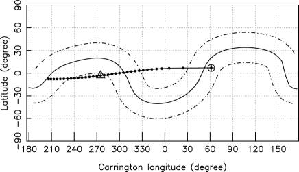
Figure 1: The current sheet as determined by the WSO with the “classic” extrapolation to a source surface at 2.5 $R_{\odot}$ is shown as a heavy solid line. The location of the slow wind belt ($\pm 20^{\circ}$ about the current sheet) is indicated by dashed lines. The path to PSR J1022+1001 on 2006 Aug 25 at 00:20 UT has been extrapolated back to the source surface along the streamlines assuming radial flow and a velocity of 400 km/s. The source-surface point corresponding to the point of closest approach to the Sun along the line of sight is indicated by a triangle and that corresponding to the Earth position by $\oplus$. The furthest point from the Earth which is shown subtends an angle of 85^∘ at the Sun.

However the location of the current sheet is subject to some error because a current-free potential-field model was used to extrapolate the photospheric observations of the WSO into the corona. Also the width of the slow wind belt is not well-defined and the density may vary with time. In this work we are concerned with the effect of these modeling errors on the final magnetic field estimate, and how these can be reduced using the additional constraint provided by a simultaneous group delay measurement. This was suggested by Ord et al. (2007), but they were unable to measure the group delay with sufficient accuracy in their observations. We do not have enough measurements to make a strong statement about the magnetic field of the solar wind, other than to show consistency with other measurements, but we have sufficient data to show the modeling errors one can expect and to compare them with statistical errors. In the following sections we will discuss: the observations and the primary analysis; the coronal model and the fitting process; the magnetic fields estimates and their sensitivity to model errors; and the prospects for future such observations.

2 Observations and Primary Analysis

The observations were part of the Parkes Pulsar Timing Array (PPTA) project which commenced in 2004 and has made observations of 20 MSPs at intervals of 2-3 weeks since then (Manchester, 2008). Here we restrict our analysis to the pulsar which provides the best observations for our purpose, PSR J1022$+$1001 which has ecliptic latitude $b_{e}=-0.06^{\circ}$, but two other MSPs regularly observed with the PPTA, J1730$-$2304 ($b_{e}=0.19^{\circ}$) and J1824$-$2452 ($b_{e}=-1.55^{\circ}$) are potentially useful. The observations analysed are those when the line of sight to PSR J1022$+$1001 happened to be close to the Sun - they were not deliberately scheduled to be near the Sun. As a result there are few observations useful for this work. All observations use the center beam of the Parkes 20-cm Multibeam receiver (Staveley-Smith et al., 1996) at frequencies close to 1400 MHz. All of the data were recorded in full-polarization mode. The back-end signal processing systems are Parkes digital filter bank systems (PDFB1 to PDFB4). Each observation has a total bandwidth of 256 MHz with 1024 channels. The duration of each observation is 64 minutes and the data were averaged with 1-min sub-integrations. A 2-min pulsed calibration signal was recorded before each pulsar observation. The flux density scale was set using observations of Hydra A. The cross-coupling between feed probes was measured using observations of PSR J0437$-$4715 covering a wide range of hour angles.

The primary analysis was done using PSRCHIVE software (Hotan et al., 2004). Initially, 5% of the band edges and radio frequency interference (RFI) were automatically removed. Then the data were flux- and polarization-calibrated and the cross-coupling between the feed polarizations was corrected using the pac/pcm algorithm in PSRCHIVE. In pulsar analysis the group delay is quantified by the “dispersion measure” DM which is the path integrated electron density in pc cm^-3. The Faraday rotation is quantified by the “rotation measure” RM, which is the term in square brackets in equation 1 in units of rad m^-2. We will use these measures in our further discussion.

The method of obtaining RM is similar to that discussed in Yan et al. (2011). We approached the final result with a series of three successive approximations. We first adjusted the RM to optimize the linearly polarized intensity integrated over the bandwidth. Then we separated each observation into upper and lower halves of the total band. An improved value of RM was determined using the weighted mean of position angle difference between the two halves of the band for each pulse phase bin. The RM also includes a time variable ionospheric component. We corrected it using an ionospheric model which is encoded in 2007 International Reference Ionophere (IRI) model. It was relatively small, ranging from $-$0.45 to $-$2.25 rad m^-2, but not negligible.

To obtain the final approximation to RM we used the corrected position angle vs pulse phase measured far from the Sun by Yan et al. (2011) as a reference template. We then found a weighted average of the differences of each observation near the Sun to this reference template. The normalized chi-squared of these weighted averages was typically about 1.3, indicating that the error estimates used in the weighted fit were reasonably accurate and the position-angle template was a good model when the pulsar was near the Sun.

To estimate the DM contribution from the solar wind, we used a simpler procedure. The DM variations due to the interstellar medium for PSR J1022$+$1001 are smaller than the measurement error (You et al., 2007b). So we simply estimated pulse arrival times in the normal way, by fitting a detailed timing model to the entire set of observations, excluding those near the Sun. We then obtained DM_⊙ by comparing the observed timing residual near the Sun with this distant average. There is a contribution from the ionosphere but, unlike the RM contribution, the ionospheric DM contribution is negligible compared with the measurement error.

The final RM and DM measurements used are summarized in Table 1 and plotted in Figure 2 vs distance from the Sun.

Table 1: Observations of the PSR J1022$+$1001 near the Sun. The ecliptic coordinates are $b_{e}=-0.06^{\circ}$ and $l_{e}=153.9^{\circ}$.

Date	UT	$R_{0}$	$I$	$L/I$	RM⊙	DM⊙
		(R⊙)	(mJy)	(%)	(rad m-2)	(10-3cm-3pc)
2005/08/29	02:15	7.5	3.0 $\pm$0.3	62	$-11.6\pm 0.15$	$3.6\pm 0.8$
2006/08/24	03:40	$-$11.3	8.0 $\pm$0.4	52	$-0.72\pm 0.06$	$1.2\pm 0.3$
2006/08/25	00:20	$-$8.2	4.6 $\pm$1.0	48	$-1.49\pm 0.24$	$0.3\pm 2.0$
2006/08/28	23:49	6.2	13.3 $\pm$1.3	58	$-23.3\pm 0.09$	$8.2\pm 0.6$
2006/08/30	00:02	9.9	12.4 $\pm$0.7	52	$-3.9\pm 0.05$	$3.6\pm 0.3$
2006/08/31	01:19	13.7	2.3 $\pm$0.4	54	$0.34\pm 0.16$	$2.0\pm 1.3$
2008/08/31	23:41	19.0	1.1 $\pm$0.2	48	$-0.18\pm 0.17$	$5.6\pm 0.9$
2009/08/30	02:01	11.2	3.2 $\pm$0.2	55	$0.17\pm 0.08$	$7.7\pm 0.4$

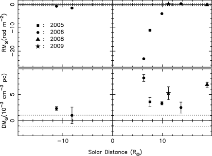
Figure 2: Observations of PSR J1022+1001 near the Sun. The abscissa is the distance from the Sun. The E limb data is plotted with a negative distance, and the W limb data with a positive distance. The observations for different years are marked by different symbols. The error bars on the RM are smaller than the symbol size.

3 Solar wind model fitting

We assume that the electron density is bimodal, as noted earlier. The average density in the two modes has been estimated (Guhathakurta & Fisher, 1995, 1998; Muhleman & Anderson, 1981; Allen, 1947); we use the same approximations as were used by You et al. (2007a). The density $n_{e}$ in the fast wind is

$$n_{e}(R)=(1.155R^{-2}+32.2R^{-4.39}+3254R^{-16.25})10^{11}\;{\rm m}^{-3}$$ (3)

and $n_{e}$ in the slow wind is

$$n_{e}(R)= (4.1R^{-2}+23.53R^{-2.7})10^{11}+$$ (4)

$$(1.5R^{-6}+2.99R^{-16})10^{14}\;{\rm m}^{-3}.$$

Here $R$ is the distance from the center of the Sun in $R_{\odot}$. To match the DM observations we scale the electron density by a factor F, and to minimize the number of free parameters we use the same factor in both the fast and slow wind.

We assume that the slow wind belt is centered on the current sheet as determined by the WSO photospheric observations extrapolated into the corona (McComas et al., 2000). However the width of the slow wind belt is variable and not precisely determined in any case (Mancuso & Spangler, 2000). Accordingly we have tested models with widths of $\pm 10^{\circ}$, $\pm 20^{\circ}$ and $\pm 30^{\circ}$.

The extrapolation is done with three similar, but subtly different, techniques referred to as: “classic”; “radial 250”; and “radial 325” in the WSO data base. The three models find a potential solution which is current free and radial at some source surface. The radial models both constrain the photospheric field to be radial and differ only in the source surface which is at 2.50 or 3.25 $R_{\odot}$. The classic model does not constrain the photospheric field to be radial but requires a somewhat ad hoc polar field correction. It assumes a source surface at 2.5 $R_{\odot}$. We assume that the magnetic field is the same in the fast and slow wind, that it is radial, and that it varies quadratically with solar distance. We take the polarity of the magnetic field from the corresponding WSO model.

To provide an idea of the range of the extrapolation models and a comparison with other solar wind observations, we plot the current sheets for the three models over the solar wind velocity measurements for 2006 from the STELAB in Figure 3. Here one can see that the three extrapolation models vary significantly in the maximum latitude extent of the current sheet, and that the width of the slow velocity belt is not clearly defined.

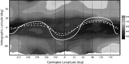
Figure 3: Solar wind velocity from STELAB, Nagoya U. This figure has been rotated in longitude to match Figure 1. The current sheet locations from the three WSO models have been overlaid. The “classic” model is a solid line, the “radial 250” model is dashed, and the “radial 325” model is dot-dashed.

It is helpful to examine the integrand of the path integrals to see where the maximum contributions arise. For numerical purposes we transform the path integral into an integral over the angle subtended at the Sun. This makes the range finite and compresses the integrand in a useful way. The integrands for group delay and Faraday rotation for the path shown in Figure 1 are shown in Figure 4. One can see that the contributions from the slow dense wind are dominant in both integrands and the location of the current sheet is very important in obtaining the Faraday rotation.

                                   

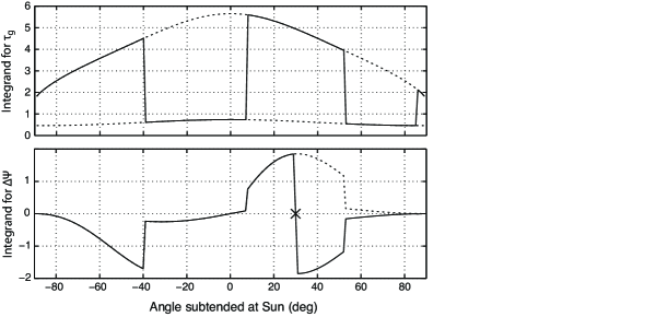
Figure 4: Integrands for group delay (top panel) and Faraday rotation (bottom panel) for the path shown in Figure 1. The integrands for fast and slow wind alone are shown dashed in the top panel. The integrand for Faraday rotation if the phase reversal at the current sheet were not present is shown dashed in the lower panel. The $\times$ marks the point near Carrington longitude $310\degr$ where the line of sight crosses the current sheet (cf. Figure 1).

The fitting procedure consists of three steps. First, we examine the LASCO C3 movies on the three days surrounding the observations and confirm that there was no obvious transient during the observing period. This was true of all the observations in Table 1. Second, we calculate the DM from one of the 9 models (3 extrapolation methods and 3 widths of the slow wind belt) and find the factor F necessary to match the observed DM in each case. Third, we use that factor F and an arbitrary $|B|$ to calculate the RM for that model, and scale $|B|$ until the model matches the observed RM. The DM and RM steps are repeated for all 9 models.

There were three observations that we could not model completely in this way. In one case, 2006 Aug 25, the DM measurement is not adequate to determine the factor F, so we set F=1. In the second case, 2009 Aug 30, all three models showed that the path was entirely in the slow wind. The electron density was 20% above its average (F = 1.2), but the RM was very small - within 2 $\sigma$ of zero. This would be expected if the path did not cross the current sheet. Two of the three extrapolation models indicated that the path would cross the current sheet and give a significant RM, but the third, the “radial 250” model did not indicate a current sheet crossing so the predicted RM = 0. In this case we have a consistent model but no estimate of the magnetic field. In the third case, 2008 Aug 31, all three models show that the path is almost entirely in the slow wind. The electron density was high (F = $3.4\pm 0.4$) and the RM was very small. The “radial 325” model predicted the wrong sign of RM indicating a significant error in the location of the current sheet. The “classic” model predicted $|B|=0.2\pm 0.2$ mG and the “radial 250” model $|B|=59\pm 56$ mG. We doubt that $|B|<0.4$ mG at 11.2 R_⊙ and suggest that the “radial 250” model is more consistent with the observation.

The results for the nine different models are shown in Table 2. One can see that the factor F varies from 0.5 to 3.0, which confirms that having simultaneous DM observations provides a strong constraint on the solar wind model. We have taken the mean of the 9 estimates of $|B|$ for each observation as the best estimate of $|B|$ for a given observation. The rms of these 9 estimates is a measure of the model sensitivity of that particular estimate. We also have an estimate of the statistical error derived from propagation of the errors on the primary measurements of DM and RM. These statistical errors are dominated by the error in measuring DM. Finally we find the $|B|$ estimate that would have been made in the absence of DM observations simply by setting F = 1 for each model and recalculating $|B|$. This summary is shown in Table 3. Here one can see that the model errors (merr) exceed the statistical (sterr) errors in every case, and the average effect of correcting for the observed DM substantially exceeds the model errors.

Table 2: Results of model sensitivity analysis using 3 WSO models and 3 widths for slow wind. Here $|B|$ in mG is estimated at the point where the line of sight is closest to the Sun.

Observation	mod	$\pm 10^{\circ}$		$\pm 20^{\circ}$		$\pm 30^{\circ}$
		F	$|B|$	F	$|B|$	F	$|B|$
2005/08/29	clas	0.9	48.9	0.6	33.1	0.5	26.6
02:16 UT	250	0.9	29.6	0.6	23.2	0.5	20.0
7.5 $R_{\odot}$	325	0.8	23.7	0.5	19.3	0.5	19.0
2006/08/28	clas	3.0	24.2	2.1	21.9	1.3	19.8
23:49 UT	250	2.7	21.8	1.4	17.2	0.9	14.8
6.2 $R_{\odot}$	325	2.4	20.8	1.3	16.4	0.8	15.0
2006/08/30	clas	2.3	12.0	1.4	12.7	1.0	10.4
00:02 UT	250	1.7	10.2	1.0	8.2	0.7	6.5
9.9 $R_{\odot}$	325	1.8	8.4	0.9	7.4	0.6	6.7
2006/08/25	clas	1.0	14.1	1.0	3.5	1.0	2.7
20:56 UT	250	1.0	28.5	1.0	3.4	1.0	3.4
$-8.2R_{\odot}$	325	1.0	10.6	1.0	2.3	1.0	1.2

Table 3: Final estimates of $|B|$ at the point where the line of sight is closest to the Sun. $|B|$ is given both corrected by measured DM and uncorrected. The measured DM exceeds that expected from the electron density model by the factor F.

Observation	$R_{0}$	$|B|$ (mG)				F
	($R_{\odot}$)	DMcor	uncor	merr	sterr	mean	merr	sterr
2005/08/29	7.5	27.0	42.3	$\pm 9.5$	$\pm 6.7$	0.64	$\pm 0.17$	$\pm 0.14$
2006/08/28	6.2	19.1	12.3	$\pm 3.4$	$\pm 1.4$	1.77	$\pm 0.80$	$\pm 0.13$
2006/08/30	9.9	9.2	8.0	$\pm 2.3$	$\pm 1.1$	1.27	$\pm 0.57$	$\pm 0.11$
2006/08/25	$-8.2$		7.7	$\pm 8.9$	$\pm 1.5$	1.0

4 Discussion of results

We have identified four primary contributions to the error on magnetic field estimates made using the Faraday rotation technique. In order of importance these are: failure to correct for DM variations ($\approx$50%); inaccuracy of estimation of the current sheet location ($\approx$25%); error in the DM measurement ($\approx$15%); and error in the Faraday rotation estimate ($\approx$1%). Thus use of simultaneous DM observations can roughly double the precision of the magnetic field estimates. The value of the PPTA for such measurements is clear. It provides a good timing model for the DM far from the Sun and a good template for the position-angle variations far from the Sun.

We have plotted our estimates of $|B|$ along with those of other authors in Figure 5. The estimates of Ord et al. (2007) and Smirnova et al. (2009) are not plotted because in both cases the authors only provide a measurement of the average line-of-sight component of the magnetic field and do not attempt to estimate $|B|$. Their estimates of the average line-of-sight components are consistent with other observations but do not put a useful constraint on $|B|$. Our estimates of $|B|$ are somewhat lower than the others, but are consistent with them, within the error bars. All the observations are broadly consistent with the Helios space craft measurements and an extrapolation like $R^{-2}$. Thus our measurements, although few in number, confirm the very important result that the potential field models of the corona seriously underestimate the magnitude of the magnetic field for $R>5R_{\odot}$.

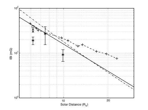
Figure 5: Magnetic field observations near the Sun. The measurements in Table 3 are plotted as * symbols with error bars. The extrapolated Helios measurements are a solid line (Burlaga, 2001), an average of the Patzold et al. (1987) observations ($|B|=1000(6R^{-3}+1.18R^{-2})$ mG) are a dot-dashed line and the observations of Gopalswamy & Yashiro (2011) are + symbols connected by a dashed line. The observation of Spangler (2005) is an open box and the range given by Ingleby et al. (2007) is a pair of connected x symbols.

We did not observe any transients near the Sun and would not have been able to analyze them with the technique we used. However it might be possible to do so if sufficient additional information, such as might be provided by STEREO, were available to constrain the geometry of the magnetic field. We note that Faraday rotation is capable of 1% precision by itself, and one might be able to measure rapid variations of magnetic field during transients with this accuracy.

We believe that more extensive observations of PSRs J1022$+$1001, J1730$-$2304, and J1824$-$2452 near the Sun, perhaps involving more telescopes to provide continuous coverage during the closest approach, would be valuable and should be undertaken at the next opportunity. There are five additional MSPs with ecliptic latitudes $\leq 2^{\circ}$ that may be suitable for precision timing: J0030$+$0451; J1614$-$2230; J1721$-$2457; J1802$-$2124; and J1811$-$24. Preliminary observations would be required to confirm that these are “good timers” before undertaking coronal measurements. The cluster of pulsars with a right ascension close to 18:00 would facilitate an intensive observing program in the last two weeks of December each year, but there are insufficient MSPs to monitor the corona on a regular basis.

References

- Allen (1947) Allen C. W., 1947, MNRAS, 107, 426
- Altschuler & Newkirk (1969) Altschuler M. D., Newkirk G., 1969, Solar Phys., 9, 131
- Bird & Edenhofer (1990) Bird M. K., Edenhofer P., 1990, Remote Sensing Observations of the Solar Corona. p. 13
- Bird et al. (1994) Bird M. K., Volland H., Paetzold M., Edenhofer P., Asmar S. W., Brenkle J. P., 1994, ApJ, 426, 373
- Burlaga (2001) Burlaga L. F., 2001, Planetary and Space Science, 49, 1619
- Gopalswamy & Yashiro (2011) Gopalswamy N., Yashiro S., 2011, ApJ, 736, L17+
- Guhathakurta & Fisher (1998) Guhathakurta M., Fisher R., 1998, ApJ, 499, L215+
- Guhathakurta & Fisher (1995) Guhathakurta M., Fisher R. R., 1995, Geophys. Res. Lett., 22, 1841
- Guhathakurta et al. (1996) Guhathakurta M., Holzer T. E., MacQueen R. M., 1996, ApJ, 458, 817
- Hollweg et al. (1982) Hollweg J. V., Bird M. K., Volland H., Edenhofer P., Stelzried C. T., Seidel, B. L., 1982, J. Geophys. Res., 87, 1
- Hotan et al. (2004) Hotan A. W., van Straten W., Manchester R. N., 2004, PASA, 21, 302
- Ingleby et al. (2007) Ingleby L. D., Spangler S. R., Whiting C. A., 2007, ApJ, 668, 520
- Jensen et al. (2005) Jensen E. A., Bird M. K., Asmar S. W., Iess L., Anderson J. D., Russell C. T., 2005, Adv. Space Res., 36, 1587
- Levy et al. (1969) Levy G. S., Sato T., Seidel B. L., Stelzried C. T., Ohlson J. E., Rusch W. V. T., 1969, Science, 166, 596
- Manchester (2008) Manchester R. N., 2008, in C. Bassa, Z. Wang, A. Cumming, & V. M. Kaspi ed., 40 Years of Pulsars: Millisecond Pulsars, Magnetars and More Vol. 983 of American Institute of Physics Conference Series, The Parkes Pulsar Timing Array Project. pp 584–592
- Mancuso & Spangler (1999) Mancuso S., Spangler S. R., 1999, ApJ, 525, 195
- Mancuso & Spangler (2000) Mancuso S., Spangler S. R., 2000, ApJ, 539, 480
- McComas et al. (2000) McComas D. J., Barraclough B. L., Funsten H. O., Gosling J. T., Santiago-Muñoz E., Skoug R. M., Goldstein B. E., Neugebauer M., Riley P., Balogh A., 2000, J. Geophys. Res., 105, 10419
- Muhleman & Anderson (1981) Muhleman D. O., Anderson J. D., 1981, ApJ, 247, 1093
- Ord et al. (2007) Ord S. M., Johnston S., Sarkissian J., 2007, Solar Phys., 245, 109
- Patzold et al. (1987) Patzold M., Bird M. K., Volland H., Levy G. S., Seidel B. L., Stelzried C. T., 1987, Solar Phys., 109, 91
- Sakurai & Spangler (1994a) Sakurai T., Spangler S. R., 1994a, ApJ, 434, 773
- Sakurai & Spangler (1994b) Sakurai T., Spangler S. R., 1994b, Rad. Sci., 29, 635
- Schatten et al. (1969) Schatten K. H., Wilcox J. M., Ness N. F., 1969, Solar Phys., 6, 442
- Smirnova et al. (2009) Smirnova T. V., Chashei I. V., Shishov V. I., 2009, Astronomy Reports, 53, 252
- Spangler (2005) Spangler S. R., 2005, Space Sci. Rev., 121, 189
- Staveley-Smith et al. (1996) Staveley-Smith L., Wilson W. E., Bird T. S., Disney M. J., Ekers R. D., Freeman K. C., Haynes R. F., Sinclair M. W., Vaile R. A., Webster R. L., Wright A. E., 1996, PASA, 13, 243
- Yan et al. (2011) Yan W. M., Manchester R. N., van Straten W., Reynolds J. E., Hobbs G., Wang N., Bailes M., Bhat N. D. R., Burke-Spolaor S., Champion D. J., Coles W. A., Hotan A. W., Khoo J., Oslowski S., Sarkissian J. M., Verbiest J. P. W., Yardley D. R. B., 2011, MNRAS, 414, 2087
- You et al. (2007a) You X. P., Hobbs G. B., Coles W. A., Manchester R. N., Han J. L., 2007a, ApJ, 671, 907
- You et al. (2007b) You X. P., Hobbs G., Coles W. A., Manchester R. N., Edwards R., Bailes M., Sarkissian J., Verbiest J. P. W., van Straten W., Hotan A., Ord S., Jenet F., Bhat N. D. R., Teoh A., 2007b, MNRAS, 378, 493