Simulations of chromospheric heating by ambipolar diffusion

Abstract

We propose a mechanism for efficient heating of the solar chromosphere, based on non-ideal plasma effects. Three ingredients are needed for the work of this mechanism: (1) presence of neutral atoms; (2) presence of a non-potential magnetic field; (3) decrease of the collisional coupling of the plasma. Due to decrease of collisional coupling, a net relative motion appears between the neutral and ionized components, usually referred to as “ambipolar diffusion”. This results in a significant enhancement of current dissipation as compared to the classical MHD case. We propose that the current dissipation in this situation is able to provide enough energy to heat the chromosphere by several kK on the time scale of minutes, or even seconds. In this paper, we show that this energy supply might be sufficient to balance the radiative energy losses of the chromosphere.

1 Introduction

The degree of plasma ionization in the lower solar atmosphere $-$ photosphere and chromosphere $-$ is very small. Using VAL-C model atmosphere as a reference (Vernazza et al. 1981), the abundance of ionized atoms, relative to neutral atoms, is as low as $10^{-4}$ at heights of temperature minimum, and it remains always well below unity even at larger heights. In addition to that, the collisional coupling of the plasma becomes less important with height. A simple calculation reveals that cyclotron frequency of hydrogen ions may exceed the collisional frequency already in the lower photosphere, for values of magnetic field strength expected for the quiet photosphere, see Figure 1.

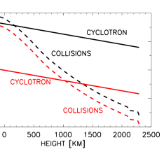
Figure 1.: Estimation of the collisional and cyclotron frequencies for electrons (black lines) and hydrogen ions (red lines) in the photosphere and chromosphere of the Sun. The magnetic field strength is assumed to vary with height as $B(z)=B_{0}\exp{(-z/H_{B})}$, with $B_{0}=100$ G and $H_{B}=600$ km.

These two factors may lead to a break of the assumption underlying magnetohydrodynamics (MHD) and lead to new effects, not taken into account in the classical approach, as ambipolar diffusion. In astrophysics, ambipolar (or neutral) diffusion usually refers to the decoupling of neutral and charged components. Ambipolar diffusion causes the magnetic field to diffuse through neutral gas due to collisions between neutrals and charged particles, the latter being frozen-in into the magnetic field.

There is an increasing number of evidences for the importance of deviations from MHD in different situations. The presence of neutral atoms in partially ionized plasmas significantly affects wave excitation and propagation (Kumar & Roberts 2003; Khodachenko et al. 2004, 2006; Forteza et al. 2007; Vranjes et al. 2008; Soler et al. 2009, 2010; Zaqarashvili et al. 2011). It is also important for magnetic reconnection (Brandenburg & Zweibel 1994, 1995; Sakai et al. 2006; Smith & Sakai 2008; Sakai & Smith 2009). Non-ideal plasma effects can modify the equilibrium balance of photospheric flux tubes (Khodachenko & Zaitsev 2002) and chromospheric structures, such as prominences (Arber et al. 2009; Gilbert et al. 2002). Another phenomenon potentially affected by non-ideal plasma effects is magnetic flux emergence (Leake & Arber 2006; Arber et al. 2007). Despite this increasing evidence, we are far from a complete understanding of the influence of these effects.

In this paper, we continue the investigation started in Khomenko & Collados (2012). There, we studied the consequences of the ambipolar diffusion into the heating of the magnetized solar chromosphere. In the presence of neutrals, the ambipolar (or neutral) diffusion is orders of magnitude larger than the classical Ohmic diffusion, leading to efficient Joule dissipation of electric currents. Our calculations have demonstrated that just by existing relatively weak (10–40 G), non-force-free magnetic fields, the chromospheric layers above 1000 km can be efficiently heated by current dissipation reaching an increase of temperature of 1-2 kK in a time interval of minutes. The work of ambipolar diffusion would stop when all the atoms become ionized or when the magnetic field becomes force-free ($\vec{J}\parallel\vec{B}$). We proposed that this heating mechanism may be efficient enough to balance the radiative losses of the chromosphere (see Khomenko & Collados 2012). Here we explore this possibility by including the radiative damping in our initial calculations.

2 Equations and numerical solution

We solve numerically the quasi-MHD equations of conservation of mass, momentum, internal energy, and the induction equation (Khomenko & Collados 2012).

$$\frac{\partial\rho}{\partial t}+\vec{\nabla}\left(\rho\vec{u}\right)=0$$ (1)

$$\rho\frac{D\vec{u}}{Dt}=\vec{J}\times\vec{B}+\rho\vec{g}-\vec{\nabla}p$$

$$\frac{1}{(\gamma-1)}\frac{Dp}{Dt}+\frac{\gamma}{(\gamma-1)}p\vec{\nabla}\vec{u}=\eta\mu_{0}\vec{J^{2}}+\eta_{A}\mu_{0}\vec{J_{\bot}^{2}}+Q_{\rm rad}$$

$$\frac{\partial\vec{B}}{\partial t}=\vec{\nabla}\times\left[(\vec{u}\times\vec{B})-\eta\mu_{0}\vec{J}-\eta_{A}\mu_{0}\vec{J_{\bot}}\right]$$

where the following definitions are used:

$$\rho=\sum_{\alpha=n,i,e}\rho_{\alpha};\,\,\,\vec{u}={1\over\rho}\sum_{\alpha=n,i,e}(\rho_{\alpha}\vec{u}_{\alpha});\,\,\,\vec{J}=en_{e}(\vec{u}_{i}-\vec{u}_{e});\,\,\,p=\sum_{\alpha=n,i,e}p_{\alpha}$$ (2)

and $\vec{J}_{\perp}$ is the component of the current perpendicular to the magnetic field. These equations are produced by summing up the equations for three different species (electrons ($e$), hydrogen ions ($i$) and neutral hydrogen ($n$)). When deriving them we neglected the non-diagonal components of the pressure tensor and assumed that the diffusion velocities $\vec{w}_{\alpha}=\vec{u}-\vec{u}_{\alpha}$ ($\alpha=e,i,n$) are small, neglecting terms containing $w_{\alpha}^{2}$. In the Ohm’s law we neglected the time variation of relative ion-neutral velocity $\vec{u}_{i}-\vec{u}_{e}$, the effects on the currents by partial pressure gradients of the three species, and the gravity force acting on electrons. The Hall term of the Ohm’s law does not appear in the energy equation and, consequently, has no impact on the thermal evolution of the system. For consistency, we removed the Hall term from the induction equation as well. The Ohmic and ambipolar diffusion coefficients are equal to:

$$\eta=\frac{m_{e}(\nu_{ei}+\nu_{en})}{e^{2}n_{e}\mu_{0}};\,\,\,\eta_{A}=\frac{(\rho_{n}/\rho)^{2}|B|^{2}}{(\rho_{i}\nu_{in}+\rho_{e}\nu_{en})\mu_{0}}$$ (3)

and the collisional frequencies are:

$$\nu_{in}=n_{n}\sqrt{\frac{8k_{B}T}{\pi m_{in}}}\sigma_{in};\,\,\,\nu_{en}=n_{n}\sqrt{\frac{8k_{B}T}{\pi m_{en}}}\sigma_{en};\,\,\,\nu_{ei}=\frac{n_{e}e^{4}\Lambda}{3m_{e}^{2}\epsilon_{0}^{2}}\left(\frac{m_{e}}{2\pi k_{B}T}\right)^{3/2}$$ (4)

where $m_{in}=m_{i}m_{n}/(m_{i}+m_{n})$ and $m_{en}=m_{e}m_{n}/(m_{e}+m_{n})$. The respective cross sections are $\sigma_{in}=5\times 10^{-19}$ m² and $\sigma_{en}=10^{-19}$ m². $\Lambda$ is the Coulomb logarithm.

After subtracting the equilibrium conditions, these equation are solved by means of our code mancha (Khomenko et al. 2008; Felipe et al. 2010; Khomenko & Collados 2012) with the inclusion of the physical ohmic and ambipolar diffusion terms in the equation of energy conservation and in the induction equation. As our code propagates non-linear perturbations to the magneto-static equilibrium, we treat the diffusion terms as perturbations. The radiative losses term $Q_{\rm rad}$ in the energy equation calculated from the solution of Radiative Transfer Equation in Local Thermodynamic Equilibrium (LTE) and grey approximation for the opacity dependence on wavelength $\lambda$.

$$Q_{\rm rad}=-\int_{\lambda}(\vec{\nabla}\vec{F}_{\lambda})d\lambda;\,\,\,\vec{F}_{\lambda}=\int_{4\pi}{I_{\lambda}(\vec{\mu})\vec{\mu}d\Omega}$$ (5)

where $\vec{F}_{\lambda}$ is radiative energy flux, $I_{\lambda}$ is specific intensity, $\vec{\mu}$ marks the direction and $d\Omega$ is a solid angle. Following the philosophy of our code, we also perturb the radiative cooling term, $\Delta Q_{\rm rad}=Q_{\rm rad}-Q_{\rm rad}(0)$, the zero-order term $Q_{\rm rad}(0)$ being eliminated from the equations as a part of equilibrium condition.

The equations are solved in two spatial dimensions, though the vector quantities are allowed to have three dimensions (2.5D approximation). As the temperature and the ionization state vary with time, we recalculate the ionization balance of the atmosphere at each time step, assuming LTE (Saha equations). We then update the neutral fraction, $\rho_{n}/\rho$, needed for the calculation of the ambipolar diffusion coefficient (Eq. 3).

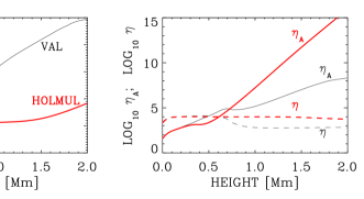
Figure 2.: Ionization fraction $\rho_{e}/\rho$ (left) and diffusion coefficients $\eta$, $\eta_{A}$ in m² s^-1 (right) as a function of height in the two flux tube models. Black thin lines: VAL-based tube; red thick lines: HOLMUL-based tube.

3 Flux tube model

In quiet regions of the solar chromosphere, diagnostic tools based on the Hanle effect point to magnetic field strengths of the order of tens Gauss (Trujillo Bueno et al. 2005; Centeno et al. 2010; Štěpán & Trujillo Bueno 2010). To simulate such non-active chromospheric conditions, we used a 2nd-order thin magnetic flux tube model as initial atmosphere (Pneuman et al. 1986; Khomenko et al. 2008). The model represents a horizontally infinite series of flux tubes that merge at some height in the chromosphere, preventing them from excessive opening with height. This magnetic field configuration is non-force-free. Here we used two flux tube models, the main difference between them is their (horizontally homogeneous) temperature structure. One has the vertical temperature structure of VAL-C (Vernazza et al. 1981), and the other has that of HOLMUL (Holweger & Mueller 1974). The magnetic field strength is similar in both cases, decreasing with height, from about 800 G in the photosphere to 35 G in the chromosphere. In the rest of the text, we will refer to these models as VAL-based and HOLMUL-based flux tubes.

While the VAL-C model atmosphere includes the chromospheric temperature increase, the temperature in the HOLMUL model monotonically decreases with height dictated by the conditions of radiative equilibrium. This peculiarity determines the ionization fraction and value of the ambipolar diffusion coefficients in the models (see Fig. 2). In the HOLMUL-based tube, the ionization fraction value does not exceed $10^{-3}$, even in the chromosphere. The values of the Ohmic diffusion coefficient $\eta$ (see Eq. 3) are similar in both models. The ambipolar diffusion $\eta_{A}$ is orders of magnitude larger than $\eta$ already above 1 Mm height. Due to the much lower ionization fraction in the HOLMUL-based model, the value of $\eta_{A}$ there significantly exceeds that of the VAL-based model. Such values of $\eta_{A}$ imply important current dissipation on very short time scales and a much quicker dissipation is expected in the cooler HOLMUL-based model.

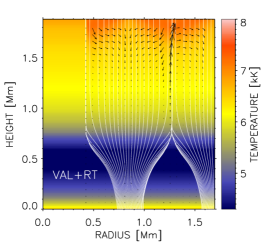
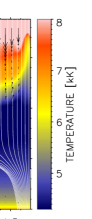
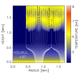
Figure 3.: Simulation snapshots after 800 s of evolution. Top left: VAL-C based flux tube with $Q_{\rm rad}=0$; top right: same but $Q_{\rm rad}\neq 0$; bottom left: HOLMUL-based flux tube with $Q_{\rm rad}=0$; bottom right: same, but $Q_{\rm rad}\neq 0$. The background color is temperature, the scale is the same for all panels. Vertical white lines are magnetic field lines. Arrows show the velocity field. For better visual comparison we keep unchanged the temperature structure from 0 to 0.42 Mm, though the variations are present in the simulations.

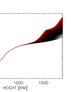
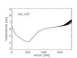
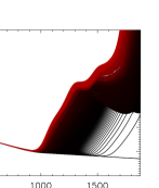
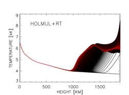
Figure 4.: Temperature as a function of height at horizontal position 0.6 Mm, see Fig. 3. Top left: VAL-C based flux tube with $Q_{\rm rad}=0$; top right: same but $Q_{\rm rad}\neq 0$; bottom left: HOLMUL-based flux tube with $Q_{\rm rad}=0$; bottom right: same, but $Q_{\rm rad}\neq 0$. Different lines are separated 1 sec in time at the upper two panels, and 0.5 sec in time at the lower two panels. Progressively more red colors indicate larger times till 800 sec since the start of the simulation.

Figure 5.: Time variations of temperature at $X=0.6$, $Z=1.8$ Mm in VAL-based flux tube (left) and HOLMUL-based flux tube (right). Dashed lines: $Q_{\rm rad}=0$; solid lines: $Q_{\rm rad}\neq 0$. First few time steps are shown by bullets, separated in time by 1 sec (left) and 0.5 sec (right).

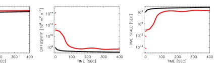
Figure 6.: Time variation of the ionization fraction $\rho_{e}/\rho$ (left); ambipolar diffusion coefficient $\eta_{A}$ (middle); and characteristic time scale $L^{2}/\eta_{A}$ (right) in the VAL-based flux tube (black) and HOLMUL-based flux tube (red), in the simulations with $Q_{\rm rad}=0$. The values at taken at $X=0.6$, $Z=1.8$ Mm. Bullets are separated 0.5 sec in time.

4 Heating of small-scale flux tubes

Here we describe four simulation runs: (i) VAL-based flux tube with $Q_{\rm rad}=0$; (ii) VAL-based flux tube with $Q_{\rm rad}\neq 0$; (iii) HOLMUL-based flux tube with $Q_{\rm rad}=0$; (iv) HOLMUL-based flux tube with $Q_{\rm rad}\neq 0$. The flux tube models are initially in magneto-static equilibrium, obtained without considering the diffusion terms. Without external perturbation, they do not evolve. After introducing the perturbation in the form of diffusion terms, we perturb the initial magnetic field structure via the induction equation. Then, as time evolves, this perturbation translates to the rest of the variables of the system and they start to change. Thanks to the Joule heating term in the energy equation ($\eta_{A}\mu_{0}J_{\bot}^{2}$, Eq. 1) the magnetic energy is efficiently converted into thermal energy, producing heat. This heat is balanced by the radiative cooling term $Q_{\rm rad}$.

Figure 3 shows snapshot from the four simulation runs 800 s after the introduction of the perturbation. At this time moment, the temperature has increased at the upper layers of the flux tubes in all simulations, but by a different amount. A more detailed view of the temperature behavior is provided in Figures 4 and 5. Fig. 4 gives the height dependence of the temperature at a fixed horizontal position inside the flux tube (X=0.6 Mm, close to flux tubes walls), for different time moments. Fig. 5 provides the time evolution of the temperature at a fixed point in the chromosphere, for all four simulations.

In all cases, the most important heating is achieved at the upper part of the domain, close to the tube borders. This behavior is expected because the term responsible for the heating ($\eta_{A}\mu_{0}J_{\bot}^{2}$) is orders of magnitude larger at these locations (see Fig. 9 in Khomenko & Collados 2012).

In the simulations with $Q_{\rm rad}=0$ (left panels of Figs. 3, 4) the relative temperature increase, achieved after 800 sec, is significantly larger in the cooler HOLMUL model. In the VAL-based model, the temperature at 1.8 Mm reaches 8200 K after 800 sec of the simulation, which is $\sim$1600 K above its initial value. In the HOLMUL-based model, it reaches 12000 K, i.e. $\sim$8200 K above its initial value. This disparity in the amount of heating is readily understood given the order-of-magnitude different $\eta_{A}$ values (Fig. 2). The temperature is visibly enhanced above $1-1.2$ Mm height. At these heights the action of the ambipolar diffusion becomes important in our model.

There is a large difference in the time scale of heating between the VAL-base and HOLMUL-based models. We can roughly define a time scale as $L^{2}/\eta_{A}$, setting a characteristic spatial scale of the system to $L=10^{5}$ m. Figure 6 shows temporal variations of the time scale in the VAL-based and HOLMUL-based models. It also shows variations of the ionization fraction and $\eta_{A}$. In the HOLMUL-based model the characteristic time scale is initially as low as $10^{-4}$ sec, producing an almost immediate increase of the temperature from 3700 K to 5700 K (Fig. 5, bullets on the right panel). This temperature rise causes an increase of the ionization fraction from $10^{-3}$ to $\sim 0.5$, and a drop of the $\eta_{A}$ some three orders of magnitude at the first few seconds. After the initial rapid variation, the evolution becomes smoother, with characteristic times around 100 sec. Note that VAL-based model does not show such quick changes at the beginning of the simulation, since $\eta_{A}$ is initially much smaller than in the HOLMUL-based model.

While the temperature constantly increases in the simulations with $Q_{\rm rad}=0$, there is an oscillatory-like balance established in the simulations with $Q_{\rm rad}\neq 0$ (Fig. 4, right panels; Fig. 5, solid lines). After an initial increase, we observe damped oscillations of temperature converging to some constant value. For example, at the location $X=0.6$, $Z=1.8$ Mm, the value of temperature to which the simulations converge is 7100 K (VAL-based, 500 K above the initial value), and 6000 K (HOLMUL-based, 2300 K above the initial value). Thus, keeping in mind all the approximations and simplifications of our modeling, we conclude that the Joule heating and radiative cooling terms in the energy equation can balance each other.

5 Conclusions

We have performed numerical simulations showing that the solar chromosphere can be effectively heated due to the Joule dissipation of electric currents, enhanced in the presence of neutral atoms (ambipolar diffusion). Our main conclusions are:

• The amount of heating and its time scale depend on the initial temperature of chromospheric magnetic structures. In cooler regions the heating can act extremely rapidly, reaching a temperature increase of 2 kK in few seconds time, while in the hotter regions the heating time scale is of the order of minutes.

• The Joule heating by ambipolar diffusion may be able to balance radiative losses of the chromosphere. Our simulations show that after a period of damped oscillations, the temperature stabilizes at some constant value. In the particular case of the simulations considered here this value is $6-7$ kK at 1.8 Mm.

Acknowledgments

This work is partially supported by the Spanish Ministry of Science through projects AYA2010-18029 and AYA2011-24808. This work contributes to the deliverables identified in FP7 European Research Council grant agreement 277829, “Magnetic connectivity through the Solar Partially Ionized Atmosphere”, whose PI is E. Khomenko (Milestone 4 and contribution toward Milestone 1).

References

- Arber et al. (2009) Arber, T. D., Botha, G. J. J., & Brady, C. S. 2009, ApJ, 705, 1183
- Arber et al. (2007) Arber, T. D., Haynes, M., & Leake, J. E. 2007, ApJ, 666, 541
- Brandenburg & Zweibel (1994) Brandenburg, A., & Zweibel, E. G. 1994, ApJ, 427, L91
- Brandenburg & Zweibel (1995) — 1995, ApJ, 448, 734
- Centeno et al. (2010) Centeno, R., Trujillo Bueno, J., & Asensio Ramos, A. 2010, ApJ, 708, 1579
- Felipe et al. (2010) Felipe, T., Khomenko, E., & Collados, M. 2010, ApJ, 719, 357
- Forteza et al. (2007) Forteza, P., Oliver, R., Ballester, J. L., & Khodachenko, M. L. 2007, A&A, 461, 731
- Gilbert et al. (2002) Gilbert, H. R., Hansteen, V. H., & Holzer, T. E. 2002, ApJ, 577, 464
- Holweger & Mueller (1974) Holweger, H., & Mueller, E. A. 1974, Solar Phys., 39, 19
- Khodachenko et al. (2004) Khodachenko, M. L., Arber, T. D., Rucker, H. O., & Hanslmeier, A. 2004, A&A, 422, 1073
- Khodachenko et al. (2006) Khodachenko, M. L., Rucker, H. O., Oliver, R., Arber, T. D., & Hanslmeier, A. 2006, Advances in Space Research, 37, 447
- Khodachenko & Zaitsev (2002) Khodachenko, M. L., & Zaitsev, V. V. 2002, Ap&SS, 279, 389
- Khomenko & Collados (2012) Khomenko, E., & Collados, M. 2012, ApJ, in press
- Khomenko et al. (2008) Khomenko, E., Collados, M., & Felipe, T. 2008, Solar Phys., 251, 589
- Kumar & Roberts (2003) Kumar, N., & Roberts, B. 2003, Solar Phys., 214, 241
- Leake & Arber (2006) Leake, J. E., & Arber, T. D. 2006, A&A, 450, 805
- Pneuman et al. (1986) Pneuman, G. W., Solanki, S. K., & Stenflo, J. O. 1986, A&A, 154, 231
- Sakai & Smith (2009) Sakai, J. I., & Smith, P. D. 2009, ApJ, 691, L45
- Sakai et al. (2006) Sakai, J. I., Tsuchimoto, K., & Sokolov, I. V. 2006, ApJ, 642, 1236
- Smith & Sakai (2008) Smith, P. D., & Sakai, J. I. 2008, A&A, 486, 569
- Soler et al. (2009) Soler, R., Oliver, R., & Ballester, J. L. 2009, ApJ, 699, 1553
- Soler et al. (2010) — 2010, A&A, 512, A28
- Trujillo Bueno et al. (2005) Trujillo Bueno, J., Merenda, L., Centeno, R., Collados, M., & Landi Degl’Innocenti, E. 2005, ApJ, 619, L191
- Štěpán & Trujillo Bueno (2010) Štěpán, J., & Trujillo Bueno, J. 2010, ApJ, 711, L133
- Vernazza et al. (1981) Vernazza, J. E., Avrett, E. H., & Loeser, R. 1981, apj, 45, 635
- Vranjes et al. (2008) Vranjes, J., Poedts, S., Pandey, B. P., & de Pontieu, B. 2008, A&A, 478, 553
- Zaqarashvili et al. (2011) Zaqarashvili, T. V., Khodachenko, M. L., & Rucker, H. O. 2011, A&A, 529, A82