Order-disorder transition in a model with two symmetric absorbing states

Abstract

We study a model of two-dimensional interacting monomers which has two symmetric absorbing states and exhibits two kinds of phase transition; one is an order-disorder transition and the other is an absorbing phase transition. Our focus is around the order-disorder transition, and we investigate whether this transition is described by the critical exponents of the two-dimensional Ising model. By analyzing the relaxation dynamics of “staggered magnetization,” the finite-size scaling, and the behavior of the magnetization in the presence of a symmetry-breaking field, we show that this model should belong to the Ising universality class. Our results along with the universality hypothesis support the idea that the order-disorder transition in two-dimensional models with two symmetric absorbing states is of the Ising universality class, contrary to the recent claim [K. Nam et al., J. Stat. Mech.: Theory Exp. (2011) L06001]. Furthermore, we illustrate that the Binder cumulant could be a misleading guide to the critical point in these systems.

I introduction

During recent decades, intense theoretical efforts have been devoted to classifying absorbing phase transitions (APTs) and, as a result, several universality classes have been found (for a review, see, e.g., Refs. Marro and Dickman (1999); Hinrichsen (2000); Ódor (2004); Lübeck (2004)). Although a firmly established classification principle is still desired, symmetry is unequivocally expected to play an important role in determining universality classes. On the one hand, if a model which has a single absorbing state and which does not have extra symmetry or conservation laws exhibits an APT, it is argued that this model should belong to the directed percolation (DP) universality class Janssen (1981); Grassberger (1982). On the other, many systems with two symmetric (sets of) absorbing states are known to form another universality class. Such examples with $Z_{2}$ symmetry are the probabilistic cellular automata model Grassberger et al. (1984), the interacting monomer-dimer (IMD) model Kim and Park (1994), the nonequilibrium kinetic Ising model Menyhárd (1994), and the interacting monomer-monomer model with infinitely many absorbing states Park and Park (2001), to cite only a few.

Although symmetry seems important, there are also some systems with $Z_{2}$ symmetry which do not share criticality with the above-mentioned models. Such exceptions can be found in Ref. Park and Park (2009). Hence, symmetry alone is not sufficient to determine the universality class and further studies are necessary to determine a guiding principle in terms of symmetry.

The starting point to develop a principle would be construction of a (coarse-grained) field theory for each universality class, followed by a renormalization group analysis. The connection between DP and the reggeon field theory has been clarified long time ago Cardy and Sugar (1980) (see also Janssen (1981); Grassberger (1982)). Endeavors have also been made to formulate a field theory for systems with $Z_{2}$-symmetric absorbing states. Cardy and Täuber Cardy and Täuber (1996, 1998) developed the field theory for the branching annihilating random walks with even numbers of offspring (BAWE) Takayasu and Tretyakov (1992), which has mod-2 conservation of particle number. Since $Z_{2}$ symmetry entails the mod-2 conservation of domain walls in one dimension, the BAWE in one dimension belongs to the same universality class as systems with two symmetric absorbing states. The mod-2 conservation, however, has nothing to do with the $Z_{2}$ symmetry in higher dimensions. In particular, the BAWE in higher dimensions shows trivial transitions Cardy and Täuber (1996, 1998), which is not the case for two-dimensional models with $Z_{2}$ symmetry Droz et al. (2003); Al Hammal et al. (2005); Vazquez and López (2008); Nam et al. (2011). In this regard, the field theory of the BAWE cannot be a coarse-grained description for models with $Z_{2}$ symmetry in $d$ dimensions. Thus, there was a theoretical request to develop a field theory with $Z_{2}$ symmetry in higher dimensions and, as a response, a phenomenological Langevin equation was introduced Al Hammal et al. (2005) (see also Ref. Canet et al. (2005) for an analysis of the corresponding field theory by the nonperturbative renormalization group method).

Recently, however, this phenomenological Langevin equation description has been challenged Nam et al. (2011). The Langevin equation predicts that there are in general two transitions in two dimensions; an order-disorder transition which is concomitant with the $Z_{2}$ symmetry breaking (SB) and an APT (see Ref. Droz et al. (2003) for the first observation of two transitions in a microscopic model). Numerical analysis of the Langevin equation revealed Al Hammal et al. (2005) that the $Z_{2}$ SB transition is of the Ising class and the APT is of the DP class. Although a Monte Carlo simulation of the two-dimensional IMD model also found a $Z_{2}$ SB transition followed by an APT, it was claimed that the critical behavior for the $Z_{2}$ SB transition is not of the Ising class Nam et al. (2011). In fact, no Monte Carlo simulations studies up to now, to our knowledge, have clearly shown that the $Z_{2}$ SB occurring in a system with two symmetric absorbing states is described by the Ising critical exponents, which was the motivation of Ref. Nam et al. (2011). If the claim in Ref. Nam et al. (2011) turns out to be true, a different coarse-grained description from that suggested is called for. Even more seriously, the conclusion in Ref. Nam et al. (2011) questions the validity of the theory that any continuous $Z_{2}$ SB transition between ordered and disordered phases should be described by the scalar $\phi^{4}$ theory Grinstein et al. (1985), which was the motivation to introduce the model-$A$ type (according to the Hohenberg-Halperin classification scheme Hohenberg and Halperin (1977)) interaction to the Langevin equation Al Hammal et al. (2005).

Hence, it is necessary to study the $Z_{2}$ SB transition exhibited by a two-dimensional model with two symmetric absorbing states more extensively to make a firm conclusion concerning the universality class. In this paper, we thoroughly investigate the SB transition. The model studied in this paper will be called the two dimensional interacting monomers (2DIM) model which is a two-dimensional version of the model studied in Ref. Park and Park (2008).

The paper is organized as follows: After introducing a model and appropriate order parameters in Sec. II, we present numerical analysis of the SB transition in Sec. III. Section IV discusses the claim in Ref. Nam et al. (2011), studies the absorbing phase transition to confirm the DP transition, and then summarizes the paper.

II Model

The 2DIM model is defined on a square lattice with size $L^{2}$ ($L$ is assumed to be even). Every site is indexed by a two dimensional vector $\bm{x}=(i,j)$ with integer components $i$ and $j$ ($i,j=0,1,\ldots,L-1$). Periodic boundary conditions are assumed. For later purposes, the lattice is subdivided into two sublattices $E$ and $O$. The sublattice $E$ ($O$) is defined as a set of sites $\bm{x}=(i,j)$ with $i+j$ even (odd). Each site is either occupied by a monomer or vacant. Two monomers are not allowed to occupy a single site at the same time. Each site is given a state variable $a_{\bm{x}}$ which takes the value 1 (0) if site ${\bm{x}}$ is occupied (vacant). A configuration is characterized by state variables at all sites.

The dynamic rules are as follows: A monomer attempts to adsorb on a randomly chosen vacant site (called a target site). Depending on the number $n$ of occupied nearest neighbors of the target site, the fate of the monomer will be different. If $n=0$, the monomer adsorbs with rate 1. On the other hand, if $n\neq 0$, the monomer adsorbs with rate $n\lambda_{n}$, but the adsorbed monomer immediately forms a dimer with a randomly chosen monomer among $n$ monomers on the nearest neighbor sites, and the dimer is desorbed in no time. Effectively, an adsorption event on a vacant site with occupied nearest neighbors removes one monomer from the lattice. If all nearest neighbors of the target site are occupied, that is, if $n=4$, a monomer is not allowed to adsorb on the target site, which amounts to setting $\lambda_{4}$ to zero. Since $\lambda_{4}=0$, any configuration with all vacant sites surrounded by monomers is an absorbing state.

To write the master equation for the above dynamics in a succinct way, we introduce a mathematical notation; for any configuration $C$ with the state variable $a_{\bm{y}}$ for every site $\bm{y}$, $C_{\bm{x}}$ stands for the configuration obtained by changing the state variable at site $\bm{x}$ to $1-a_{\bm{x}}$ and by keeping all other state variables the same as in $C$. Using this notation, the master equation can be written as

$$\frac{d}{dt}P(C;t)=\sum_{\bm{x}}\left[W_{CC_{\bm{x}}}P(C_{\bm{x}};t)-W_{C_{\bm{x}}C}P(C;t)\right],$$ (1)

with the transition rate

$$W_{C_{\bm{x}}C}=\delta_{a_{\bm{x}},0}\delta_{n_{\bm{x}},0}+\delta_{a_{\bm{x}},1}\sum_{\bm{y}}{}^{\prime}\sum_{k=1}^{3}\lambda_{k}\delta_{a_{\bm{y}},0}\delta_{n_{\bm{y}},k},$$ (2)

where $\sum{}^{\prime}$ means the sum over nearest neighbor vectors $\bm{y}$ of site $\bm{x}$, $a_{\bm{x}}$ ($a_{\bm{y}}$) is the state variable at site $\bm{x}$ ($\bm{y}$) in the configuration $C$, $n_{\bm{x}}$ ($n_{\bm{y}}$) means the number of occupied nearest neighbors of site $\bm{x}$ ($\bm{y}$) in $C$, and $\delta$ is the Kronecker delta symbol. By observing that $(C_{\bm{x}})_{\bm{x}}=C$, one can easily find the transition rate $W_{CC_{\bm{x}}}$.

To simulate the master equation, we have used the following algorithm. First, we make a list of vacant sites with at least one vacant nearest neighbor. For convenience, we will refer to such a vacant site as an active site. Assume that there are $N_{t}$ active sites at time $t$. A target site out of $N_{t}$ active sites is selected at random with equal probability. If all nearest neighbors of the target site are vacant, it becomes occupied with probability $\Delta t$ which is defined as

$$\Delta t=\frac{1}{\textrm{max}(1,\lambda_{1},2\lambda_{2},3\lambda_{3})}.$$ (3)

If the target site has $n$ occupied nearest neighbors ($n=1$, 2, or 3), a configuration change can occur with probability $n\lambda_{n}\Delta t$. If a change is destined, one monomer out of $n$ is selected with equal probability and it is removed from the system, which mimics the dimer desorption explained above. After the above attempt, time increases by $\Delta t/N_{t}$ and the list of active sites is updated in an appropriate way. We repeat the above procedure until $t$ exceeds a preassigned maximum observation time or no active site exists in the system. For convenience, we set $\lambda_{1}=2\lambda_{2}=3\lambda_{3}=\lambda$ in what follows and study phase transitions by tuning $\lambda$.

Now we will specify the initial condition studied in this paper. At $t=0$, the sublattice $O$ is empty, but a site in the sublattice $E$ is occupied with probability $m_{0}$ ($0\leq m_{0}<1$). With this initial condition, there are only two absorbing states; the sublattice $E$ is fully occupied and the sublattice $O$ is empty, or vice versa. In this sense, absorbing states have perfect ‘anti-ferromagnetic’ order. The absorbing state with the sublattice $E$ ($O$) filled with monomers will be called the even (odd) absorbing state.

Since we expect two transitions (an APT and a $Z_{2}$ SB transition), two quantities that are respectively called the density of active sites and the ‘staggered magnetization’ will be measured during simulations.

The density of active sites at time $t$ is defined as

$$\phi(t,L)\equiv\frac{1}{L^{2}}\sum_{\bm{x}}\delta_{a_{\bm{x}},0}(1-\delta_{n_{\bm{x}},4}),$$ (4)

where $n_{\bm{x}}$ is the number of occupied nearest neighbors of site $\bm{x}$ in a configuration at time $t$. If the system is in one of the two absorbing states at time $t$, $\phi(t,L)$ is obviously zero. We define the (averaged) density of active sites in the thermodynamic limit as

$$\rho(t)\equiv\lim_{L\rightarrow\infty}\langle\phi(t,L)\rangle,$$ (5)

where $\langle\ldots\rangle$ stands for the average over all independent realizations.

The staggered magnetization (SM) is defined as

$${\cal M}(t,L)\equiv\frac{1}{L^{2}}\left[\sum_{\bm{x}\in E}-\sum_{\bm{x}\in O}\right]\left[2a_{\bm{x}}(t)-1\right].$$ (6)

If the system is in the even (odd) absorbing state, the SM is ${\cal M}(t,L)=1$ ($-1$). The (averaged) SM at time $t$ in the thermodynamic limit is defined as

$$m(t)\equiv\lim_{L\rightarrow\infty}\langle{\cal M}(t,L)\rangle.$$ (7)

Figure 1: Phase diagram of the 2DIM model. $\lambda_{c}$ is the transition point of the order-disorder transition and $\lambda_{a}$ is that of the absorbing phase transition.

Since the initial condition gives

$$\left\langle a_{\bm{x}}\right\rangle=\begin{cases}0&\text{ if }\bm{x}\in O,\\ m_{0}&\text{ if }\bm{x}\in E,\end{cases}$$ (8)

$$\left\langle\delta_{a_{\bm{x}},0}\left(1-\delta_{n_{\bm{x}},4}\right)\right\rangle=\begin{cases}1-m_{0}^{4}&\text{ if }\bm{x}\in O,\\ 1-m_{0}&\text{ if }\bm{x}\in E,\end{cases}$$ (9)

we get

$$\langle{\cal M}(0,L)\rangle=m_{0},\quad\langle\phi(0,L)\rangle=1-\frac{1}{2}m_{0}\left(1+m_{0}^{3}\right).$$ (10)

Note that with the above initial condition, $m(t)$, which is defined in the thermodynamic limit, will remain positive for all finite $t$ if $0<m_{0}<1$ and the order-disorder phase transition is defined by the infinite-time limit of $m(t)$ such that

$$\mathfrak{M}\equiv\lim_{t\rightarrow\infty}m(t)=\begin{cases}\text{nonzero,}&\text{ordered phase,}\\ 0,&\text{disordered phase.}\end{cases}$$ (11)

As we will see later, the 2DIM model exhibits two transitions: an order-disorder transition occurring at $\lambda=\lambda_{c}$ and an absorbing phase transition occurring at $\lambda=\lambda_{a}<\lambda_{c}$. The schematic phase diagram is depicted in Fig. 1.

III Numerical analysis of the order-disorder transition

In this section, we present the simulation results, focusing on the order-disorder transition. Rather than studying the Binder cumulant, we analyze how $m(t)$ approaches the steady state value. This approach is also known as the nonequilibrium relaxation method Ozeki and Ito (2007).

At criticality, the SM is expected to decay as Suzuki (1985); Nam et al. (2008)

$$m(t)\sim t^{-\beta/(\nu z)},$$ (12)

with the critical exponents $\beta$, $\nu$, and $z$ defined as,

$$\mathfrak{M}\sim(\lambda_{c}-\lambda)^{\beta},\quad\xi\sim|\lambda_{c}-\lambda|^{-\nu},\quad\tau\sim|\lambda_{c}-\lambda|^{-\nu z},$$ (13)

where $\lambda_{c}$ is the critical point, $\xi$ is the correlation length, and $\tau$ is the relaxation time. For the two dimensional Ising model, $\beta=\frac{1}{8}$ and $\nu=1$ are known exactly (see, for instance, Ref. Baxter (1982)), but $z\simeq 2.17$ Nam et al. (2008) is known only numerically; nonetheless it serves well for our purpose. In simulations, we set $m_{0}=0.9$ (initial condition) and observed how $\langle{\cal M}(t,L=2^{11})\rangle$ behaves up to $t=5\times 10^{5}$. When we study the finite-size scaling later, the finite size effect is argued to be negligible up to the observation time in this case, so $\langle{\cal M}(t,L=2^{11})\rangle$ can be regarded as $m(t)$.

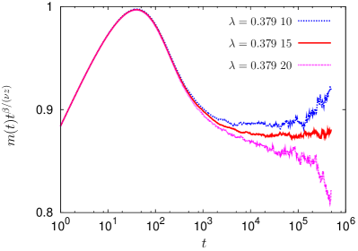
Figure 2: (Color online) Plots of $m(t)t^{\beta/(\nu z)}$ vs $t$ with Ising critical exponents $\beta=\frac{1}{8}$, $\nu=1$, and $z=2.17$ for $\lambda=0.379~{}10$, 0.379 15, and 0.379 20 (from top to bottom) on a semilogarithmic scale.

In Fig. 2, we depict the behavior of $m(t)t^{\beta/(\nu z)}$ for three different values of $\lambda$ as a function of $t$ on a semilogarithmic scale, using the critical exponents of the two-dimensional Ising model. The numbers of independent simulation runs for $\lambda=0.3791$, 0.379 15, and 0.3792 are 280, 912, and 160, respectively. In the ordered (disordered) phase, the curve is expected to veer up (down), and at criticality the curve should be flat, if the correct exponents are used. Thus, Fig. 2 supports the idea that the order-disorder transition in the 2DIM model is of the Ising type with the critical point $\lambda_{c}=0.379~{}15(5)$, where the number in parentheses indicates the error of the last digit.

Note that the power-law behavior of $m(t)$ is observable only for $t>10^{4}$, which implies that the 2DIM model has stronger corrections to scaling than the two-dimensional Ising model (for example, Fig. 1 in Ref. Nam et al. (2008) shows that the two-dimensional Ising model is already in the scaling regime from $t=10$). As we will see later, the strong corrections to scaling also plague the behavior of the Binder cumulant, which will be given as the reason why previous studies could not successfully report the universal value of the Binder cumulant (see Sec. IV.2).

To have further support for the Ising critical behavior, we also studied the finite size scaling. At criticality, scaling collapses for the magnetization ${\cal M}$ and for the absolute value of the magnetization $|{\cal M}|$ are expected with the scaling forms

$$\langle{\cal M}(t,L)\rangle=L^{-\beta/\nu}f(t/L^{z}),$$ (14)

$$\langle|{\cal M}(t,L)|\rangle=L^{-\beta/\nu}g(t/L^{z}),$$ (15)

where $f$ and $g$ are (universal) scaling functions. To check the finite-size scaling at criticality, we simulated the systems with sizes of $L=2^{7}$, $2^{8}$, $2^{9}$, and $2^{10}$. The numbers of independent simulation runs for $L=2^{7}$, $2^{8}$, $2^{9}$, and $2^{10}$ are 160 000, 40 000, 10 000, and 2504, respectively. The resulting scaling collapse is presented in Fig. 3 which indeed shows a nice collapse of $\langle{\cal M}(t,L)\rangle$ onto a single curve when the Ising critical exponents are employed. The scaling collapse is also nice for the average of the absolute value of ${\cal M}$ (inset of Fig. 3).

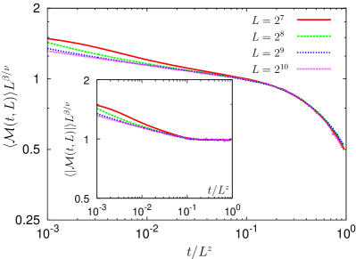
Figure 3: (Color online) Plots of $\langle{\cal M}(t,L)\rangle L^{\beta/\nu}$ vs $t/L^{z}$ with Ising critical exponents at criticality on a double logarithmic scale. Inset: Plots of $\langle|{\cal M}(t,L)|\rangle L^{\beta/\nu}$ vs $t/L^{z}$ at $\lambda=\lambda_{c}$.

As a by-product of the finite-size scaling, we can estimate the time after which the finite-size effect becomes significant to be $t\approx 0.1L^{z}$ (about $1.5\times 10^{6}$ for $L=2^{11}$) and, in turn, we affirm that the relaxation dynamics of $m(t)$ is faithfully presented in Fig. 2.

Furthermore, we also studied how the symmetry-breaking field $h$ affects the behavior of the magnetization at criticality. Like the Ising model, the SM at the critical point is supposed to behave as Nam et al. (2008)

$$m(t)=h^{1/\delta}H(th^{\nu z/(\beta\delta)}),$$ (16)

where $\delta=15$ for the two-dimensional Ising model Baxter (1982) and $H$ is a universal scaling function. It is worth while to investigate a scaling collapse of $m(t)h^{-1/\delta}$ plotted as a function of $th^{\nu z/(\beta\delta)}$, using the Ising critical exponents. Note that for the two-dimensional Ising model $\nu z/(\beta\delta)\approx 1.16$.

To introduce the symmetry-breaking field, we follow the idea in Ref. Hwang et al. (1998). Now the transition rates take the form

$$W_{C_{\bm{x}}C}= \left(1-\frac{1-(-1)^{i+j}}{2}h\right)\delta_{a_{\bm{x}},0}\delta_{n_{\bm{x}},0}$$ (17)

$$+\delta_{a_{\bm{x}},1}\sum_{\bm{y}}{}^{\prime}\sum_{k=1}^{3}\frac{\lambda}{k}\delta_{a_{\bm{y}},0}\delta_{n_{\bm{y}},k},$$

where $i$ and $j$ are components of the lattice vector $\bm{x}$ and $0<h<1$. Recall that we have set $k\lambda_{k}=\lambda$ for $k=1,2,3$. By Eq. (17), adsorption on the sublattice $E$ is more probable than on the sublattice $O$, which eventually breaks the symmetry between even and odd absorbing states.

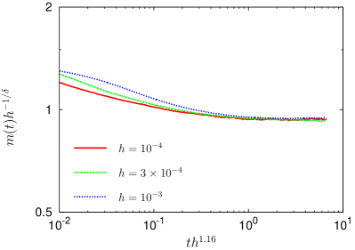
Figure 4: (Color online) Scaling collapse plot of $m(t)h^{-1/\delta}$ as a function of $th^{1.16}$ on a double logarithmic scale with the Ising critical exponent $\delta=15$.

With these modified transition rates, we simulated a system with size $L=2^{9}$ at $\lambda=\lambda_{c}$ for different values of $h$. In actual simulations, we have only to change the probability of adsorption on a vacant site in the sublattice $O$ without occupied nearest neighbors to $(1-h)\Delta t$. The resulting scaling plot is depicted in Fig. 4 which shows a nice scaling collapse. It again supports the idea that the 2DIM model should belong to the Ising universality class. To make sure that the finite-size effect is negligible, we also studied systems with size $L=2^{8}$ and obtained almost same figure as Fig. 4 (not shown here).

IV Discussion and Summary

Up to now, we have shown that the critical behavior of the order-disorder transition in the 2DIM model is of the Ising class. In this section, we will discuss the behavior of the density of active sites $\rho(t)$ and the Binder cumulant at the order-disorder transition point $\lambda_{c}$, which will be compared with the similar studies in Ref. Nam et al. (2011). Also, to confirm the universality, we discuss the critical behavior of the absorbing phase transition.

IV.1 Behavior of $\rho$ and its fluctuation at $\lambda=\lambda_{c}$

In Ref. Nam et al. (2011), diverging fluctuation of the order parameter of the absorbing phase transition was suspected to be a possible reason why the two dimensional IMD model should not belong to the Ising class. However, this order parameter, in our case $\phi$ defined in Eq. (4), seems related to the energy density of the Ising model in that $\phi$ is measured as a correlation between nearest neighbors. Since the fluctuation of the (Ising) energy is the specific heat which diverges logarithmically at criticality in two dimensions, it is actually plausible that the fluctuation of $\phi$ (times system size) diverges at criticality even though the 2DIM model belongs to the Ising class.

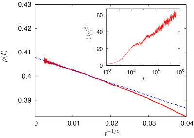
Figure 5: (Color online) Plots of $\rho(t)$ vs $t^{-1/z}$ with the Ising dynamic exponent $z=2.17$ at criticality. The straight line is the result of a linear function fitting. Inset: Plots of $(\delta\rho)^{2}$ vs $t$ at $\lambda=\lambda_{c}$ on a semilogarithmic scale.

To confirm that $\rho(t)=\langle\phi\rangle$ indeed is linked to the (average) energy density of the Ising model, we analyze how $\rho(t)$ behaves at the order-disorder transition point. Since the energy at criticality approaches the steady-state value in a power-law fashion with exponent $(\nu d-1)/(\nu z)$ Nam et al. (2008), $\rho(t)$ is expected, if it is indeed related to the energy, to approach the steady-state value $\rho^{*}$ in such a way that

$$\rho^{*}-\rho(t)\sim t^{-(\nu d-1)/(z\nu)}\approx t^{-1/z},$$ (18)

where we have set $\nu=1$ (the Ising critical exponent) and $d=2$. Hence if $\rho(t)$ is plotted as a function of $t^{-1/z}$, the curve becomes straight for small $t^{-1/z}$ and approaches $\rho^{*}$ as $t^{-1/z}\rightarrow 0$ (equivalently, $t\rightarrow\infty$). As Fig. 5 reveals, $\rho$ approaches the ordinate as a straight line for $t^{-1/z}<0.02$, as anticipated. Note that the time $t^{-1/z}=0.02$ roughly corresponds to $t=5\times 10^{3}$ after which $m(t)$ enters the scaling regime (see Fig. 2).

We also analyzed how the fluctuation of the active site density defined as

$$\left(\delta\rho\right)^{2}\equiv\lim_{L\rightarrow\infty}L^{2}\left(\langle\phi(t,L)^{2}\rangle-\langle\phi(t,L)\rangle^{2}\right)$$ (19)

behaves at $\lambda=\lambda_{c}$. The inset of Fig. 5 shows logarithmic behavior of $(\delta\rho)^{2}$ as in the two-dimensional Ising model.

Thus, we conclude that the active site density $\phi(t,L)$ is indeed associated with the energy of the Ising model. Actually, the logarithmic behavior of $(\delta\rho)^{2}$ is compatible with the slow divergence of the fluctuation observed in Ref. Nam et al. (2011).

IV.2 Binder cumulant

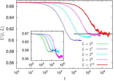
Figure 6: (Color online) Plots of $U(t,L)$ vs $t$ at criticality ($\lambda=\lambda_{c}$) on a semilogarithmic scale ($L=2^{7}$, $2^{8}$, $2^{9}$, and $2^{10}$ from left to right). As a guide to the eyes, we also plot a straight line indicating the universal Binder cumulant of the Ising universality class, 0.611. Inset: Plots of $U(t,L)$ vs $t$ in the disordered phase (at $\lambda=0.3795>\lambda_{c}$) for $L=2^{6}$, $2^{7}$, $2^{8}$, and $2^{9}$ from left to right.

Since the Binder cumulant is believed to take a universal number at criticality, we should study whether the Binder cumulant at $\lambda=\lambda_{c}$ approaches to the universal value as $L\rightarrow\infty$. Defining the Binder cumulant at time $t$ as

$$U(t,L)=1-\frac{\left\langle{\cal M}(t,L)^{4}\right\rangle}{3\left\langle{\cal M}(t,L)^{2}\right\rangle^{2}},$$ (20)

we numerically study how $U(t,L)$ behaves for different values of $L$.

In Fig. 6 we present simulation results for $U(t,L)$ for $\lambda=\lambda_{c}=0.379~{}15$ and for $\lambda=0.3795>\lambda_{c}$ (Inset). For $\lambda=0.3795$, the numbers of independent samples simulated for $L=2^{6}$, $2^{7}$, $2^{8}$, and $2^{9}$ are 200 000, 50000, 14000, and 4000, respectively and data for $\lambda=\lambda_{c}$ were collected while we studied the finite size scaling.

Since the system has absorbing states and any finite system will eventually fall into one of the absorbing states even in the active phase, there are obviously two characteristic time scales. One is $\tau_{q}$ when the system enters the quasi-stationary state and the other is $\tau_{a}$ when the system falls into one of the absorbing states. At $\lambda=\lambda_{c}$, $\tau_{q}$ diverges with system size as $\tau_{q}\sim L^{z}$, but $\tau_{a}$ should increase exponentially with $L$ because the SB transition point is in the active phase of the absorbing phase transition. Hence, to find the universal value of the Binder cumulant at the SB transition point, the observation time should be larger than $\tau_{q}$ but much smaller than $\tau_{a}$. Actually, except for the case of $L=2^{6}$, no simulation results in an absorbing state and, even for $L=2^{6}$, only $\leq 0.2\%$ of simulation runs falls into an absorbing state up to the observation time. Hence, in our analysis, the Binder cumulant is not influenced by the existence of absorbing states.

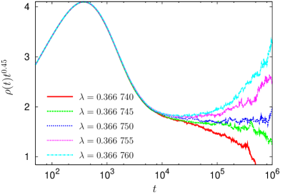
Figure 7: (Color online) Plots of $\rho(t)t^{0.45}$ vs $t$ near the critical point of the absorbing phase transition on a semilogarithmic scale.

At $\lambda=\lambda_{c}$, $U(t,L)$ in the (quasi-)stationary state increase with system size but shows a clear signature of saturating behavior to the universal number 0.611 Kamieniarz and Blöte (1993) as $L\rightarrow\infty$. Note that if the system size is not large enough, the Binder cumulant could miidetify the critical point. The unexpected behavior of the Binder cumulant should be attributed to the strong corrections to scaling already observed in Fig. 2.

The inset of Fig. 6 depicts the behavior of $U(t,L)$ at $\lambda=0.3795>\lambda_{c}$ (disordered phase). If the system size is not larger than $L=2^{8}$, one may conclude that the critical point is around 0.3795, with the value of the Binder cumulant around 0.59, which is comparable to the value reported in Ref. Nam et al. (2011). Hence we conclude that the critical point reported in Ref. Nam et al. (2011) is actually in the disordered phase.

IV.3 Absorbing phase transition

Finally, we discuss the critical behavior of the absorbing phase transition. Since the symmetry is already broken, it is expected that the model should belong to the DP class Droz et al. (2003); Al Hammal et al. (2005). To confirm this, we study the system with the initial SM $m_{0}=0.1$. In Fig. 7, we plot $\rho(t)t^{0.45}$ as a function of $t$ on a semilogarithmic scale, where $0.45$ is the critical exponent of the DP class. For $\lambda=0.366\;750$, the curve becomes flat from around $t=5\times 10^{4}$. In the active (absorbing) phase, the curves veer up (down) as usual. Thus we conclude that the critical point of the absorbing transition is $\lambda_{a}=0.366\;750(5)$ and the critical behavior is of the DP class.

Note that exponential decay of $\rho$ in the absorbing phase is observed in Fig. 7, which might look inconsistent with the power-law decay in the whole absorbing phase reported in Ref. Nam et al. (2011). However, there is a clear distinction. Since the initial SM is nonzero in our case, coarsening has not played any role. Indeed, we also observe power-law behavior in the absorbing phase if $m_{0}$ is set to zero just as in Ref. Nam et al. (2011) (data not shown).

IV.4 Summary

To sum up, we studied a model of two-dimensional interacting monomers, focusing on the order-disorder phase transition. Numerical analysis showed that the 2DIM model should belong to the Ising universality class, contrary to a recent claim Nam et al. (2011). We observed that analysis of the Binder cumulant is not an efficient method to find the critical point in two dimensional models with two symmetric absorbing states. We also reconfirmed that the absorbing phase transition occurring in the 2DIM model after the symmetry is broken is described by two-dimensional directed percolation.

Although we did not directly study the interacting monomer-dimer model, we believe that the conclusion in this paper should be applicable to the IMD model studied in Ref. Nam et al. (2011) because of the universality hypothesis. Since the two different models, IMD and 2DIM, have strong corrections to scaling at the symmetry-breaking transition point, unlike the Ising model, the origin of these strong corrections seems to be related to the presence of an absorbing state even for $\lambda>\lambda_{c}$ (disordered phase). If this is the case, it is an interesting question as to why and how the absorbing states affect the corrections to scaling; this is beyond the scope of the present paper and is deferred to a later presentation.