Multi-frequency polarization properties of ten quasars on deca-parsec scales at $z>3$

Abstract

Global VLBI (EVN+VLBA) polarization observations at 5 and 8.4 GHz of ten high redshift ($z>3$) quasars are presented. The core and jet brightness temperatures are found through modelling the self-calibrated uv–data with Gaussian components, which provide reliable estimates of the flux density and size of individual components. The observed high core brightness temperatures (median $T_{\rm b,\,core}=4\times 10^{11}$ K) are consistent with Doppler boosted emission from a relativistic jet orientated close to the line-of-sight. This can also explain the dramatic jet bends observed for some of our sources since small intrinsic bends can be significantly amplified due to projection effects in a highly beamed relativistic jet. We also model-fit the polarized emission and, by taking the minimum angle separation between the model-fitted polarization angles at 5 and 8.4 GHz, we calculate the minimum inferred Faraday rotation measure (RM_min) for each component. We also calculate the minimum intrinsic RM in the rest frame of the AGN (RM${}_{\rm min}^{\rm intr}$ = RM${}_{\rm min}(1+z)^{2}$), first subtracting the integrated (presumed foreground) RM in those cases where we felt we could do this reliably. The resulting mean core $|$RM${}_{\rm min}^{\rm intr}|$ is 5580 rad m^-2, with a standard deviation of 3390 rad m^-2, for four high-z quasars for which we believe we could reliably remove the foreground RM. We find relatively steep core and jet spectral index values, with a median core spectral index of $-0.3$ and a median jet spectral index of $-1.0$. Comparing our results with RM observations of more nearby Active Galactic Nuclei at similar emitted frequencies does not provide any significant evidence for dependence of the quasar nuclear environment with redshift. However, more accurate RM and spectral information for a larger sample of sources would be required before making any conclusive statements about the environment of quasar jets in the early universe.

1 Introduction

Quasars at $z>3$ and with GHz flux densities of the order of 1 Jy have luminosities of $\sim 10^{28}$ W Hz^-1, making them the most luminous, steady radio emitters in the Universe. In this paper, we present 5 and 8.4 GHz global VLBI polarization observations of ten quasars at $z>3$. There have been several recent studies of high-redshift jets on VLBI scales (e.g., Gurvits et al., 2000; Frey et al., 2008; Veres et al., 2010) but our observations are the first to explore this region of “luminosity – emitted frequency” parameter space in detail with polarization sensitivity. In the standard $\Lambda$CDM cosmology (H${}_{0}=70$ km s^-1 Mpc^-1, $\Omega_{\Lambda}=0.7$ and $\Omega_{M}=0.3$), the angular diameter distance reaches a maximum at $z\sim 1.6$ (e.g., Hogg, 1999), meaning that more distant objects actually begin to increase in apparent angular size with increasing $z$. As a consequence, the linear scale for observations of objects at $z\sim 3$ is similar to objects at $z\sim 0.7$. Therefore, our measurements allow us to study pc-scale structures at emitted frequencies of $\sim$20–45 GHz in comparison with properties of low-redshift core-dominated Active Galactic Nuclei (AGN) at 22 and 43 GHz (e.g., O’Sullivan & Gabuzda, 2009) at matching length scale and emitted frequency.

An important question we try to address with these observations is whether or not quasar jets and their surrounding environments evolve with cosmic time. Any systematic differences in the polarization properties or the frequency dependence of the polarization between high and low redshift sources would suggest that conditions in the central engines, jets, and/or surrounding media of quasars have evolved with redshift. Previous observations of high redshift quasars (e.g., Frey et al., 1997; Paragi et al., 1999) often show that these quasars can be strongly dominated by compact cores and that their extremely high apparent luminosities are likely due to large Doppler boosting, implying that their jets move at relativistic velocities and are pointed close to our line of sight. With this geometry, it is difficult to distinguish emerging jet components from the bright core. However, high resolution polarization observations have proven very effective in identifying barely resolved but highly polarized jet components, whose intensity is swamped by the intensity of the nearby core, but whose polarized flux is comparable to or even greater than that of the core (e.g., Gabuzda, 1999). Thus, polarization sensitivity can be crucial to understanding the nature of compact jets in the highest redshift quasars.

There is also some evidence that the VLBI jets of high redshift quasars are commonly bent or distorted; one remarkable case revealed by VSOP observations is of 1351-018 (Gurvits et al., 2000) where the jet appears to bend through almost $180^{\circ}$. Polarization observations can help elucidate the physical origin of these observed changes in the jet direction in the plane of the sky since the direction of the jet polarization can reflect the direction of the underlying flow. In some quasars (Cawthorne et al., 1993; O’Sullivan & Gabuzda, 2009), the observed polarization vectors follow curves in the jet, indicating that the curves are actual physical bends, while in others, remarkable uniformity of polarization position angle has been observed over curved sections of jet, suggesting that the apparent curves correspond to bright regions in a much broader underlying flow. One possible origin for bends could be collisions of the jet with denser areas in the surrounding medium as suggested, for example, in the case of the jet in the radio galaxy 4C 41. 17 (Gurvits et al., 1997). The polarization information allows us to test for evidence of such interaction, where the Faraday rotation measure (RM) and degree of polarization should increase substantially in those regions.

In Section 2, we describe our observations and the data reduction process. Descriptions of the results for each source are given in Section 3, while their implications for the jet structure and environment are discussed in Section 4. Our conclusions are presented in Section 5. We use the $S\propto\nu^{\alpha}$ definition for the spectral index.

2 Observations and Data Reduction

Ten high-redshift ($z>3$) AGN jets (listed in Table 1), which were all previously successfully imaged using global VLBI baselines, were targeted for global VLBI polarization observations at 4.99 and 8.415 GHz with two IFs of 8 MHz bandwidth at each frequency. These sources do not comprise a complete sample in any sense, and were chosen based on the previous VLBI observations of Gurvits et al. (2000), which indicated the presence of components with sufficiently high total intensities to suggest that it was feasible to detect their polarization.

The sources were observed for 24 hours on 2001 June 5 with all 10 antennas of the NRAO Very Long Baseline Array (VLBA) plus six antennas of the European VLBI Network (EVN) capable of fast frequency switching between 5 and 8.4 GHz (see Table 2 for a list of the telescopes used). The target sources were observed at alternating several-minute scans at the two frequencies. This led to practically simultaneous observations at the two frequencies with a resolution of $\sim 1.1$ mas at 5 GHz and $\sim 0.7$ mas at 8.4 GHz (for the maximum baseline of 11,200 km from MK to NT).

Table 1: Basic information for the high-redshift quasars and VLBI data presented in this paper.

(1)	(2)	(3)	(4)	(5)	(6)	(7)	(8)	(9)	(10)
Name	z	Linear Scale	Freq.	Beam	BPA	$I_{\rm total}$	$I_{\rm peak}$	$\sigma_{I,\rm{rms}}$	$L_{\nu}$
		[pc mas-1]	[GHz]	[mas$\times$mas]	[deg]	[mJy]	[mJy/bm]	[mJy/bm]	[$10^{28}$ W Hz-1]
0014$+$813	3.38	7.55	4.99	$1.10\times 0.95$	$-85.9$	861.4	583.2	0.3	2.10
			8.41	$0.95\times 0.68$	$-85.1$	645.1	445.6	0.9	1.57
0636$+$680	3.17	7.71	4.99	$1.25\times 0.91$	$-1.3$	348.8	270.0	0.3	0.76
			8.41	$0.82\times 0.62$	$5.3$	281.4	162.7	0.5	0.62
0642$+$449	3.41	7.53	4.99	$1.70\times 0.85$	$-15.6$	2248.2	1974.9	0.7	5.55
			8.41	$1.03\times 0.70$	$14.4$	2743.9	2460.4	3.9	6.77
1351$-$018	3.71	7.30	4.99	$3.51\times 1.10$	$-7.0$	788.0	662.2	0.4	2.23
			8.41	$2.07\times 0.86$	$-2.8$	594.0	534.2	1.4	1.68
1402$+$044	3.21	7.68	4.99	$3.52\times 0.95$	$-7.7$	831.7	617.4	0.5	1.86
			8.41	$2.03\times 0.75$	$-6.8$	719.7	488.2	0.3	1.61
1508$+$572	4.30	6.88	4.99	$1.23\times 0.97$	$15.2$	291.1	248.7	0.2	1.04
			8.41	$0.80\times 0.76$	$8.9$	198.3	170.3	0.5	0.71
1557$+$032	3.90	7.16	4.99	$3.81\times 0.97$	$-8.2$	287.0	249.6	0.3	0.88
			8.41	$2.06\times 0.80$	$-8.8$	255.8	239.1	1.0	0.78
1614$+$051	3.21	7.68	4.99	$3.74\times 0.98$	$-8.1$	792.9	588.9	0.5	1.77
			8.41	$1.99\times 0.80$	$-9.4$	465.0	333.6	1.0	1.04
2048$+$312	3.18	7.70	4.99	$2.17\times 1.12$	$-21.2$	547.0	192.7	1.5	1.20
			8.41	$2.06\times 0.71$	$-16.2$	539.1	253.9	0.6	1.19
2215$+$020	3.55	7.42	4.99	$3.45\times 1.03$	$-7.6$	271.0	190.6	0.2	0.71
			8.41	$2.06\times 0.71$	$-6.8$	174.3	122.6	0.3	0.46

Column designation: 1 - source name (IAU B1950.0); 2 - redshift; 3 - projected distance, in parsecs, corresponding to 1 mas on the sky; 4 - observing frequency in GHz; 5 - size of convolving beam in mas$\times$mas at the corresponding frequency for each source; 6 - beam position angle (BPA), in degrees; 7 - total flux density, in mJy, from CLEAN map; 8 - peak brightness, in mJy beam^-1; 9 - brightness rms noise, in mJy beam^-1, from off-source region; 10 - monochromatic total luminosity at the corresponding frequency in units of $10^{28}$ W Hz^-1.

Table 2: List of telescopes included in the global VLBI experiment.

Telescope Location	Code	Diameter	Comment
		[m]
EVN
Effelsberg, Germany	EB	100
Medicina, Italy	MC	32
Noto, Italy	NT	32
Toruń, Poland	TR	32	Failed
Jodrell Bank, UK	JB	25
Westerbork, Netherlands	WB	93∗
VLBA, USA
Saint Croix, VI	SC	25
Hancock, NH	HN	25
North Liberty, IA	NL	25
Fort Davis, TX	FD	25
Los Alamos, NM	LA	25	Failed
Pietown, NM	PT	25
Kitt Peak, AZ	KP	25
Owens Valley, CA	OV	25
Brewster, WA	BR	25
Mauna Kea, HI	MK	25

^∗ Equivalent diameter for the phased array, $\sqrt{14}\times 25$ m.

The data were recorded at each telescope with an aggregate bit rate of 128 Mbits/s, recorded in 8 base-band channels at 16 Msamples/sec with 2-bit sampling, and correlated at the Joint Institute for VLBI in Europe, Dwingeloo, The Netherlands. Los Alamos (LA) was unable to take data due to communication problems and Toruń (TR) also failed to take data, so both were excluded from the processing.

The 5 and 8.4 GHz VLBI data were calibrated independently using standard techniques in the NRAO AIPS package. In both cases, the reference antenna for the VLBI observations was the Kitt Peak telescope. The instrumental polarizations (‘D-terms’) at each frequency were determined using observations of 3C 84, using the task LPCAL and assuming 3C 84 to be unpolarized. The polarization angle ($2\chi=\arctan\frac{U}{Q}$) calibration was achieved by comparing the total VLBI-scale polarizations observed for the compact sources 1823+568 (at 5 GHz) and 2048+312 (at 8.4 GHz) with their polarizations measured simultaneously with the NRAO Very Large Array (VLA) at both 5 and 8.4 GHz, and rotating the VLBI polarization angles to agree with the VLA values. We obtained 2 hours of VLA data, overlapping with the VLBI data on June 6. The VLA angles were calibrated using the known polarization angle of 3C 286 at both 5 and 8.4 GHz (see AIPS cookbook, chapter 4). At 5 GHz, we found $\Delta\chi_{\rm 5\,GHz}=\chi_{\rm VLA}-\chi_{\rm VLBI}=67.5^{\circ}$ and at 8.4 GHz, $\Delta\chi_{\rm 8.4\,GHz}=\chi_{\rm VLA}-\chi_{\rm VLBI}=83.5^{\circ}$.

3 Results

Table 1 lists the 10 high-z quasars, their redshifts, the FWHM beam sizes at 5 and 8.4 GHz, the total CLEAN flux and the peak flux densities of the 5 and 8.4 GHz maps, the noise levels in the maps, and the 5 and 8.4 GHz luminosities, calculated assuming a spectral index of zero and isotropic radiation. Since the emission from these sources is likely relativistically boosted, the true luminosity is probably smaller by a factor of 10–100 (e.g., Cohen et al., 2007). Figure 1 gives an example of the sparse but relatively uniform uv coverage obtained for this experiment. The 5-GHz uv coverage for 2048+312 is shown; the 8.4 GHz is essentially identical but scaled accordingly.

The DIFMAP software package (Shepherd, 1997) was used to fit circular and/or elliptical Gaussian components to model the self-calibrated source structure. The brightness temperatures in the source frame were calculated for each component from the integrated flux and angular size according to

$$T_{b}=1.22\times 10^{12}\frac{S_{\text{total}}(1+z)}{d_{\max}d_{\min}\nu^{2}}$$ (1)

where the total flux density is measured in Jy, the FWHM size is measured in mas and the observing frequency is measured in GHz. The limiting angular size for a Gaussian component ($d_{\rm lim}$) was also calculated to check whether the component size reflects the true size of that particular jet emission region or not. From Lobanov (2005), we have

$$d_{\rm lim}=\sqrt{\frac{\ln 2}{\pi}b_{\rm max}b_{\rm min}\ln\left(\frac{\rm S/N}{{\rm S/N}-1}\right)}$$ (2)

where $b_{\rm max}$ and $b_{\rm min}$ are the major and minor axes of the FWHM beam and S/N is the signal-to-noise ratio of a particular component. In other words, component sizes smaller than this value yielded by the model-fitting are not reliable. Table 3 shows the results of the total intensity model-fitting for each source. For clarity of comparison, the component identified as the core has been defined to be at the origin, and the positions of the jet components determined relative to this position. The errors in the model-fitted positions were estimated as $\Delta r=\sigma_{\rm rms}d\sqrt{1+S_{\rm peak}/\sigma_{\rm rms}}/2S_{\rm peak}$ and $\Delta\theta=\arctan(\Delta r/r)$, where $\sigma_{\rm rms}$ is the residual noise of the map after the subtraction of the model, $d$ is the model-fitted component size and $S_{\rm peak}$ is the peak flux density (e.g., Fomalont, 1999; Lee et al., 2008; Kudryavtseva et al., 2010). These are formal errors, and may yield position errors that are appreciably underestimated in some cases; when this occurs we use a $1\sigma$ error estimate of $\pm 0.1$ beamwidths in the structural position angle of the component in question.

Polarization model fits, listed in Table 4, were found using the Brandeis VISFIT package (Roberts et al., 1987; Gabuzda et al., 1989) adapted to run in a linux environment by Bezrukovs & Gabuzda (2006). The positions in Table 4 have been shifted in accordance with our cross-identification of the corresponding intensity cores, when we consider this cross-identification to be reliable. The errors quoted for the model-fitted components are formal $1\sigma$ errors, corresponding to an increase in the best fitting $\chi^{2}$ by unity; again, we have adopted a 1$\sigma$ error estimate of $\pm 0.1$ beamwidths in the structural position angle of the component in question when the position errors are clearly underestimated.

Before constructing spectral-index maps, images with matched resolution must be constructed at the two frequencies. Since the intrinsic resolutions of the 8.4 and 5-GHz images were not very different (less than a factor of two), we achieved this by making a version of the final 8.4-GHz image with the same cell size, image size and beam as the 5-GHz image. The two images must also be aligned based on optically thin regions of the structure: the mapping procedure aligns the partially optically thick cores with the map origin, whereas we expect shifts between the physical positions of the cores at the two frequencies. When possible, we aligned the two images by comparing the positions of optically thin jet components at the two frequencies derived from model-fits to the VLBI data, or using the cross-correlation technique of Croke & Gabuzda (2008). After this alignment, we constructed spectral-index maps in AIPS using the task COMB.

In the absence of Faraday rotation, we expect the polarization angles for corresponding regions at the two frequencies to coincide; in the presence of Faraday rotation of the electric vector position angle (EVPA), which occurs when the polarized radiation passes through regions of magnetized plasma, the observed polarization angles will be subject to a rotation by RM$\lambda^{2}$, where RM is the Faraday rotation measure and $\lambda$ is the observing wavelength. We are not able to unambiguously identify the action of Faraday rotation based on observations at only two frequencies; however, Faraday rotation provides a simple explanation for differences in the polarization angles observed at the two frequencies. We accordingly calculated tentative Faraday rotation measures, $\textrm{RM}_{min}=(\chi_{\rm 5~{}GHz}-\chi_{\rm 8.4~{}GHz})/(\lambda^{2}_{\rm 5~{}GHz}-\lambda^{2}_{\rm 8.4~{}GHz})$, based on the results of the polarization model fitting,taking the minimum difference between the component EVPAs. We also constructed tentative RM maps in AIPS using the task COMB. In both cases, if Faraday rotation is operating, the derived RM values essentially represent a lower limit for the true Faraday rotation (assuming an absence of $n\pi$ rotations in the observed angles).

With our two frequencies, the n$\pi$ ambiguity in the RM corresponds to $n$ times 1350 rad m^-2. Table 4 lists the values of RM_min and the corresponding intrinsic polarization angle $\chi_{0}$, obtained by extrapolating to zero wavelength. However, we emphasize that polarization measurements at three or more wavelengths are required to come to any firm conclusions about the correct RM and $\chi_{0}$ values for these sources.

The main source of uncertainty for the RMs (apart from possible $n\pi$ ambiguities) comes from the EVPA calibration, which we estimate is accurate to within $\pm 3^{\circ}$; this corresponds to an RM error of $\pm 23$ rad m^-2 between 5 and 8.4 GHz. We have also attempted to obtain the correct sign and magnitude of the RM in the immediate vicinity of the AGNs by subtracting the integrated RMs derived from lower-frequency VLA measurements centered on our sources, obtained from the literature. Note that these represent the integrated RMs directly along the line of sight toward our sources, rather than along a nearby sight-line; the typical uncertainties in such measurements when based on observations at several frequencies near 1–2 GHz are typically no larger than about $\pm 5$ rad/m². Because of the lower resolution of these measurements and the greater prominence of the jets at lower frequencies, the polarization detected in such observations usually originates fairly far from the VLBI core, where we expect the overall RM local to the source to be negligible. Therefore, the lower-frequency integrated RMs usually correspond to the foreground (Galactic) contribution to the overall RM detected in our VLBI data, and subtracting off this value should typically help isolate the RM occurring in the immediate vicinity of the AGN. Due to the extremely high redshifts of these sources it can be very important to remove the foreground RM before estimating the intrinsic minimum RM in the source rest frame, RM${}_{\rm min}^{\rm intr}=(1+z)^{2}({\rm RM}_{\rm min}-{\rm RM}_{\rm Gal})$. Table 4 also lists ${\rm RM}_{\rm Gal}$ and RM${}_{\rm min}^{\rm intr}$ for sources which have measured integrated RMs in the literature. We take the polarization angles measured at the two frequencies to essentially be equal (negligible RM) within the errors if they agree to within $6^{\circ}$, and do not attempt to correct such angles for Galactic Faraday rotation, since there can be some uncertainty about interpreting integrated RMs as purely Galactic foreground RMs, and the subtraction of the integrated values from such small nominal VLBI RM values could lead to erroneous results in some cases.

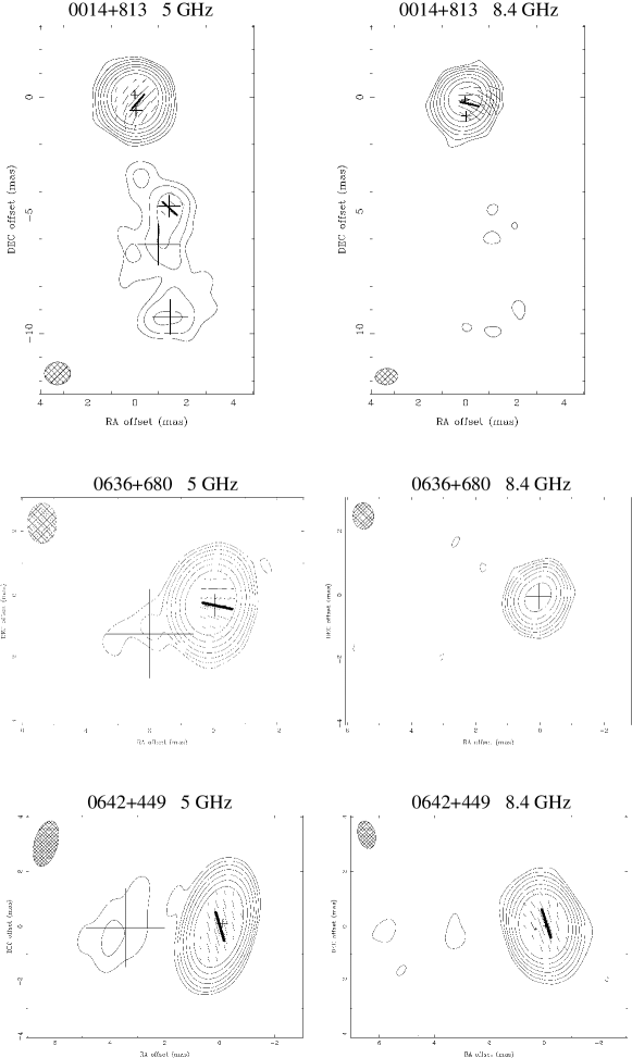
Figure 2: Total intensity ($I$) and polarization ($p$) maps for all sources at 5 GHz (left) and 8.4 GHz (right). The image axes show the relative offset from the image centre in milliarcseconds. The beamsize is indicated by an inset in each image (see Table 1 for details). The model-fitted total intensity components are indicated by the ”+” symbols while the position and angle of the polarized component model-fits are indicated by the boldface line. In all cases the contour levels increase in factors of 2 from the indicated total intensity cutoff (see Table 5). The length of the $p$ sticks represent the relative polarized intensity.

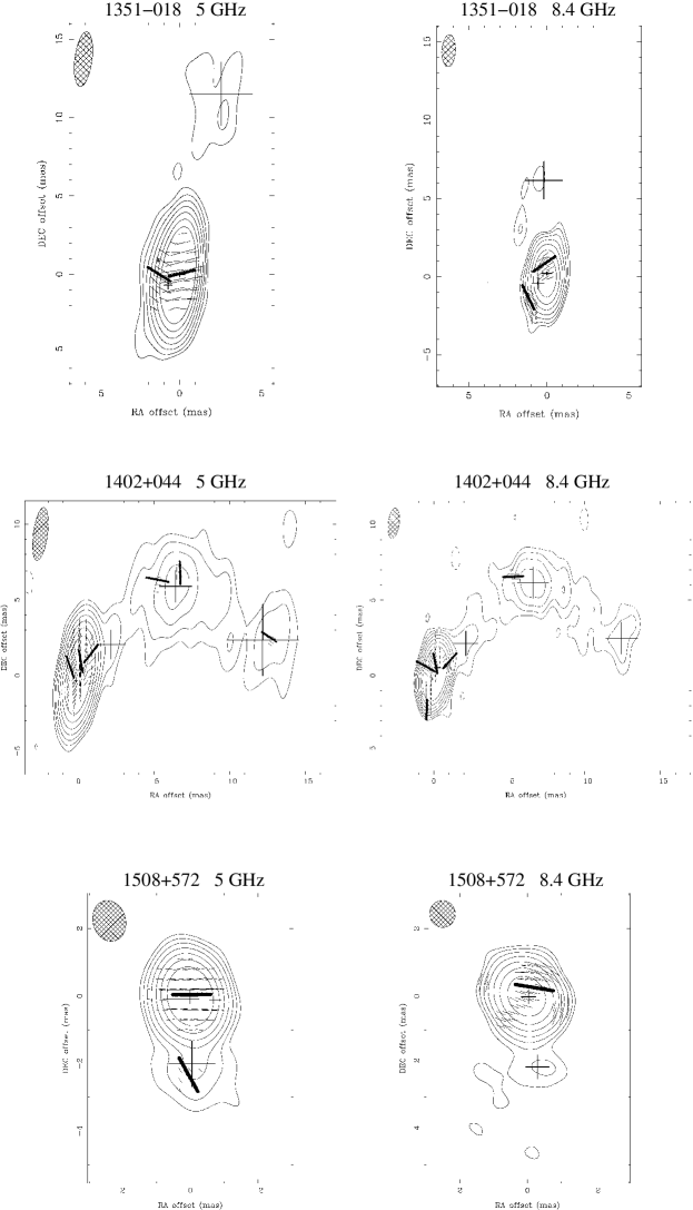
Figure 2: continued.

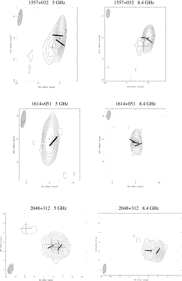
Figure 2: continued.

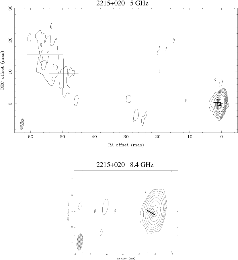
Figure 2: continued.

For each source, we present the total-intensity distributions at 5 and 8.4 GHz overlaid with EVPA sticks in Fig. 2 and also plot the positions of the model-fitted total intensity and polarization components. The derived spectral-index and RM_min distributions generally do not show unexpected features, and are not presented here; these can be obtained by contacting S.P. O’Sullivan directly.

Table 3: Total intensity model fit parameters of all sources.

(1)	(2)	(3)	(4)	(5)	(6)	(7)	(8)	(9)	(10)
Name	Freq.	Comp.	$r$	$\theta$	$I_{\rm tot}$	$d_{\rm max}$	$d_{\rm min}$	$d_{\rm lim}$	$T_{\rm b}$
	[GHz]		[mas]	[deg]	[mJy]	[mas]	[mas]	[mas]	[$\times 10^{10}$ K]
0014$+$813	4.99	A	–	–	$617\pm 20$	0.53	0.32	0.03	$78.2\pm 6.4$
		B	$0.66\pm 0.10$	$-175.7\pm 1.2$	$196\pm 11$	0.53	0.53	0.05	$15.2\pm 2.3$
		C	$4.93\pm 0.10$	$-162.8\pm 1.1$	$13\pm 3$	0.92	0.92	0.21	$0.32\pm 0.21$
		D	$6.41\pm 0.21$	$-171.0\pm 1.9$	$16\pm 4$	1.75	1.75	0.19	$0.11\pm 0.08$
		E	$9.51\pm 0.16$	$-170.9\pm 1.0$	$17\pm 4$	1.49	1.49	0.18	$0.16\pm 0.11$
	8.41	A	–	–	$547\pm 36$	0.46	0.13	0.04	$65.9\pm 11.0$
		B	$0.74\pm 0.07$	$-178.3\pm 1.7$	$85\pm 14$	0.40	0.40	0.09	$3.9\pm 1.7$
0636$+$680	4.99	A	–	–	$344\pm 15$	0.69	0.35	0.03	$28.9\pm 3.1$
		B	$2.22\pm 0.54$	$140.3\pm 9.0$	$6\pm 3$	2.76	2.76	0.23	$0.02\pm 0.02$
	8.41	A	-	-	$286\pm 21$	0.78	0.38	0.04	$7.4\pm 1.4$
0642$+$449	4.99	A	–	–	$2209\pm 60$	0.41	0.28	0.02	$417\pm 28$
		B	$3.22\pm 0.45$	$92.5\pm 7.5$	$45\pm 14$	2.86	2.86	0.15	$0.12\pm 0.11$
	8.41	A	–	–	$2313\pm 134$	0.16	0.16	0.03	$731\pm 103$
		A1	$0.20\pm 0.09$	$158.1\pm 0.8$	$458\pm 60$	0.09	0.09	0.08	$439\pm 138$
1351$-$018	4.99	A	–	–	$681\pm 23$	0.77	0.23	0.05	$89.5\pm 7.5$
		B	$1.01\pm 0.16$	$132.7\pm 1.0$	$79\pm 8$	0.48	0.48	0.14	$7.9\pm 2.0$
		C	$1.64\pm 0.12$	$56.6\pm 0.5$	$14\pm 3$	0.17	0.17	0.32	–
		D	$11.85\pm 0.59$	$-12.9\pm 2.8$	$17\pm 5$	4.02	4.02	0.30	$0.02\pm 0.02$
	8.41	A	–	–	$578\pm 37$	0.67	0.06	0.06	$125.9\pm 20.1$
		B	$0.83\pm 0.12$	$138.5\pm 9.7$	$13\pm 6$	0.76	0.76	0.40	$0.18\pm 0.19$
		C	$5.96\pm 0.63$	$-2.1\pm 5.8$	$3\pm 3$	2.43	2.43	1.06	$0.003\pm 0.008$
1402$+$044	4.99	A	–	–	$330\pm 17$	0.23	0.23	0.05	$130.0\pm 16.7$
		B	$0.76\pm 0.25$	$-24.5\pm 1.3$	$374\pm 19$	0.46	0.46	0.04	$36.9\pm 4.6$
		C	$3.33\pm 0.15$	$-44.4\pm 4.5$	$19\pm 5$	1.93	1.93	0.23	$0.11\pm 0.08$
		D	$9.07\pm 0.14$	$-46.6\pm 0.9$	$64\pm 9$	2.13	2.13	0.11	$0.29\pm 0.12$
		E	$12.64\pm 0.50$	$-77.7\pm 2.3$	$44\pm 10$	4.72	4.72	0.18	$0.04\pm 0.03$
	8.41	A	–	–	$300\pm 19$	0.14	0.14	0.07	$111.1\pm 17.5$
		B	$0.83\pm 0.16$	$-23.7\pm 1.0$	$336\pm 21$	0.43	0.43	0.06	$13.4\pm 2.1$
		C	$3.23\pm 0.29$	$-43.3\pm 5.5$	$13\pm 5$	1.62	1.62	0.27	$0.03\pm 0.04$
		D	$9.22\pm 0.20$	$-46.2\pm 1.2$	$55\pm 11$	2.07	2.07	0.15	$0.09\pm 0.05$
		E	$12.83\pm 0.32$	$-77.8\pm 1.5$	$20\pm 7$	2.09	2.09	0.18	$0.03\pm 0.03$
1508$+$572	4.99	A	–	–	$276\pm 11$	0.45	0.28	0.03	$56.1\pm 5.3$
		B	$2.00\pm 0.12$	$-178.4\pm 3.3$	$14\pm 3$	1.37	1.37	0.13	$0.20\pm 0.11$
	8.41	A	–	–	$196\pm 14$	0.42	0.14	0.03	$30.0\pm 5.2$
		B	$1.94\pm 0.14$	$-172.1\pm 3.7$	$6\pm 3$	0.70	0.70	0.20	$0.11\pm 0.13$
1557$+$032	4.99	A	–	–	$262\pm 12$	0.70	0.26	0.06	$34.0\pm 3.9$
		B	$2.64\pm 0.17$	$139.4\pm 2.4$	$14\pm 3$	1.24	1.24	0.26	$0.22\pm 0.13$
	8.41	A	–	–	$252\pm 15$	0.49	0.12	0.05	$35.0\pm 5.1$
		B	$2.16\pm 0.37$	$148.5\pm 9.2$	$15\pm 5$	2.46	2.46	0.18	$0.02\pm 0.02$
1614$+$051	4.99	A	–	–	$566\pm 24$	0.37	0.37	0.05	$63.5\pm 6.7$
		B	$1.26\pm 0.16$	$-154.4\pm 0.7$	$229\pm 15$	0.54	0.54	0.08	$12.4\pm 2.1$
	8.41	A	–	–	$347\pm 28$	0.24	0.24	0.07	$32.4\pm 6.5$
		B	$1.26\pm 0.12$	$-154.1\pm 0.7$	$117\pm 17$	0.37	0.37	0.12	$4.6\pm 1.6$
2048$+$312	4.99	A	–	–	$393\pm 38$	1.78	1.24	0.10	$3.7\pm 1.0$
		B	$1.55\pm 0.11$	$65.7\pm 2.2$	$126\pm 21$	1.43	1.43	0.17	$1.3\pm 0.6$
		C	$8.86\pm 0.36$	$56.8\pm 2.0$	$20\pm 10$	1.68	1.68	0.44	$0.14\pm 0.19$
	8.41	A	–	–	$411\pm 23$	0.80	0.44	0.04	$8.4\pm 1.2$
		B	$1.49\pm 0.07$	$80.6\pm 2.6$	$129\pm 14$	1.29	1.29	0.07	$0.56\pm 0.18$
2215$+$020	4.99	A	–	–	$141\pm 9$	0.26	0.26	0.08	$45.9\pm 7.3$
		B	$0.52\pm 0.11$	$108.0\pm 2.2$	$73\pm 7$	0.39	0.39	0.12	$10.7\pm 2.4$
		C	$1.53\pm 0.10$	$79.1\pm 5.4$	$11\pm 3$	1.26	1.26	0.30	$0.15\pm 0.10$
		D	$50.52\pm 1.52$	$79.1\pm 1.6$	$33\pm 11$	9.17	9.17	0.17	$0.009\pm 0.009$
		E	$57.71\pm 2.48$	$74.7\pm 2.3$	$19\pm 8$	11.26	11.26	0.23	$0.003\pm 0.004$
	8.41	A	–	–	$94\pm 7$	0.20	0.20	0.06	$19.0\pm 3.5$
		B	$0.50\pm 0.08$	$115.7\pm 1.3$	$66\pm 6$	0.22	0.22	0.07	$10.7\pm 2.4$
		C	$0.95\pm 0.07$	$95.5\pm 3.6$	$17\pm 3$	0.64	0.64	0.14	$0.32\pm 0.2$

Column designation: 1 - source name (IAU B1950.0); 2 - observing frequency, in GHz; 3 - component identification; 4 - distance of component from core, in mas; 5 - position angle of component with respect to the core, in degrees; 6 - total flux of model component, in mJy; 7 - FWHM major axis of Gaussian component, in mas; 8 - FWHM minor axis of Gaussian component, in mas; 9 - Minimum resolvable size, in mas; 10 - measured brightness temperature in units of $10^{10}$K.

Table 4: Polarization model fit parameters of all sources.

(1)	(2)	(3)	(4)	(5)	(6)	(7)	(8)	(9)	(10)	(11)	(12)
Name	Freq.	Comp.	$r$	$\theta$	$p$	$\chi$	$m$	RMmin	$\chi_{0}$	RMGal	RM${}_{\rm min}^{\rm intr}$
	[GHz]		[mas]	[deg]	[mJy]	[deg]	[%]	[rad m-2]	[deg]	[rad m-2]	[rad m-2]
0014$+$813	4.99	A	–	–	$4.5\pm 0.3$	$-40.9$	$1.1\pm 0.3$	384	$-120\pm 13$	$9^{a}$	$7194\pm 525$
		B	$4.72\pm 0.10$	$-163.5\pm 2.1$	$1.3\pm 0.5$	47.7	$20.0\pm 4.5$	–	–	–	–
	8.41	A	–	–	$2.3\pm 0.2$	$-92.2$	$0.7\pm 0.2$
0636$+$680	4.99	A	–	–	$4.1\pm 0.3$	78.4	$1.7\pm 0.5$	–	–	–	–
	8.41	–	–	–	–	–	–
0642$+$449	4.99	A	–	–	$21.2\pm 1.8$	15.6	$1.1\pm 0.4$	–	–	–	–
	8.41	A	–	–	$68.2\pm 4.2$	15.3	$2.6\pm 0.7$
1351$-$018	4.99	A	–	–	$5.2\pm 0.4$	$-76.2$	$0.9\pm 0.3$	$-223$	$-30\pm 6$	$-8^{a}$	$-4770\pm 599$
		B	$1.45\pm 0.11$	$100.3\pm 2.7$	$2.8\pm 0.7$	52.3	$2.7\pm 0.5$	199	$11\pm 3$	$-8^{a}$	$4592\pm 646$
	8.41	A	–	–	$4.1\pm 0.4$	$-46.4$	$0.5\pm 0.2$
		B	$2.38\pm 0.16$	$155.9\pm 2.4$	$1.7\pm 0.5$	25.7	$1.3\pm 0.4$
1402$+$044	4.99	A	–	–	$3.1\pm 0.3$	15.7	$1.8\pm 0.5$	$-199$	$57\pm 12$	–	–
		B	$0.77\pm 0.11$	$-61.5\pm 1.8$	$11.2\pm 1.1$	4.1	$2.0\pm 0.7$	$-57$	$16\pm 12$	–	–
		C	$1.50\pm 0.12$	$-60.9\pm 3.3$	$1.6\pm 0.5$	$-26.2$	$2.9\pm 0.8$	141	$-55\pm 15$	–	–
		D	$8.12\pm 0.15$	$-45.4\pm 0.9$	$1.1\pm 0.4$	83.8	$17.8\pm 5.4$	$-59$	$96\pm 49$	–	–
		E	$9.56\pm 0.14$	$-49.2\pm 1.2$	$2.0\pm 0.5$	$-1.5$	$9.1\pm 2.1$	–	–	–	–
		F	$13.41\pm 0.10$	$-81.9\pm 1.7$	$1.6\pm 0.5$	49.8	$21.2\pm 6.2$	–	–	–	–
	8.41	A1	$2.77\pm 0.20$	$177.5\pm 3.4$	$5.8\pm 0.6$	$-6.2$	$3.2\pm 0.7$
		A	–	–	$2.3\pm 0.5$	42.3	$1.5\pm 0.3$
		B	$0.54\pm 0.09$	$-60.1\pm 2.7$	$7.4\pm 0.7$	11.7	$1.3\pm 0.3$
		C	$1.48\pm 0.08$	$-72.3\pm 2.4$	$2.8\pm 0.6$	$-45.1$	$1.2\pm 0.3$
		D	$8.26\pm 0.11$	$-43.0\pm 0.9$	$2.8\pm 0.6$	91.7	$22.9\pm 9.1$
1508$+$572	4.99	A	–	–	$7.5\pm 0.9$	$-89.4$	$2.9\pm 0.8$	–	–	–	–
		B	$2.36\pm 0.18$	$177.3\pm 1.4$	$0.6\pm 0.3$	36.1	$16.9\pm 5.7$	–	–	–	–
	8.41	A	–	–	$4.0\pm 1.2$	$-93.4$	$1.3\pm 0.4$
1557$+$032	4.99	A	–	–	$3.4\pm 0.5$	54.2	$1.7\pm 0.5$	$-49$	$64\pm 40$	3a	$-1249\pm 713$
		B	$1.77\pm 0.19$	$19.5\pm 3.6$	$0.7\pm 0.3$	85.2	$1.8\pm 0.5$	68	$71\pm 32$	3a	$1561\pm 642$
	8.41	A	–	–	$3.5\pm 0.4$	60.8	$1.2\pm 0.4$
		B	$1.25\pm 0.09$	$59.1\pm 1.7$	$2.1\pm 0.3$	76.2	$6.0\pm 0.7$
1614$+$051	4.99	C	$1.51\pm 0.10$	$-95.7\pm 1.0$	$3.8\pm 0.5$	$-38.5$	$1.8\pm 0.5$	522	$-107\pm 10$	8c	$9110\pm 488$
	8.41	A	–	–	$2.9\pm 0.6$	62.4	$3.4\pm 0.7$
		B	$0.82\pm 0.08$	$-119.1\pm 2.9$	$6.5\pm 0.9$	78.7	$2.1\pm 0.4$
		C	$1.55\pm 0.09$	$-121.9\pm 3.2$	$2.6\pm 0.5$	$-69.8$	$2.0\pm 0.3$
2048$+$312	4.99	A	–	–	$3.8\pm 0.6$	$-39.5$	$3.3\pm 0.2$	–	–	–	–
		B	$2.31\pm 0.11$	$88.1\pm 1.6$	$1.1\pm 0.5$	$-61.2$	$4.7\pm 0.4$	–	–	–	–
	8.41	A	–	–	$5.5\pm 0.7$	$-35.0$	$2.2\pm 0.3$
		B	$2.04\pm 0.09$	$86.6\pm 1.9$	$1.4\pm 0.5$	$-93.6$	$6.2\pm 0.6$
2215$+$020	4.99	A	–	–	$0.6\pm 0.2$	57.0	$0.9\pm 0.4$	–	–	–	–
	8.41	A	–	–	$1.5\pm 0.4$	53.8	$1.3\pm 0.5$

Column designation: 1 - source name (IAU B1950.0); 2 - observing frequency, in GHz; 3 - component identification; 4 - distance of component from core component, in mas; 5 - position angle of component with respect to core component, in degrees; 6 - polarized flux of component, in mJy; 7 - EVPA of component, in degrees (nominal error of $\pm 3^{\circ}$ from calibration, which is much greater than any model-fit errors); 8 - Degree of polarization, in per cent, taken from a 3x3 pixel area in degree of polarization image centred on the model-fitted position; 9 - minimum rotation measure obtained from minimum separation between $\chi_{\rm 5~{}GHz}$ and $\chi_{\rm 8.4~{}GHz}$, in rad m^-2 (with nominal error of $\pm 28$ rad m^-2); 10 - intrinsic EVPA, in degrees, as corrected by RM_min. 11 - integrated (Galactic) RM, in rad m^-2, from literature ^aTaylor et al. (2009), ^bOren & Wolfe (1995). 12 - intrinsic minimum RM corrected for Galactic contribution where RM${}_{\rm min}^{\rm intr}=({\rm RM}_{\rm min}-{\rm RM}_{\rm Gal})(1+z)^{2}$.

Table 5: Total Intensity and Polarization image cutoff values.

	5 GHz		8.4 GHz
Source name	$I$ cutoff	$p$ cutoff	$I$ cutoff	$p$ cutoff
	[mJy/bm]	[mJy/bm]	[mJy/bm]	[mJy/bm]
0014$+$813	1.2	0.7	2.8	1.3
0636$+$680	0.9	0.7	1.5	0.2
0642$+$449	3.6	2.4	5.0	11.0
1351$-$018	1.3	1.1	4.0	1.3
1402$+$044	2.0	1.4	1.1	1.7
1508$+$572	1.1	0.7	1.5	1.8
1557$+$032	1.1	0.9	1.0	1.2
1614$+$051	1.7	1.1	4.2	1.5
2048$+$312	6.0	1.9	1.9	1.5
2215$+$020	0.7	0.7	1.6	0.9

3.1 0014+813

This source was discovered in the radio and classified as a flat spectrum radio quasar by Kuehr et al. (1981). Kuehr et al. (1983) obtained a redshift of 3.366, and found the source to be exceptionally bright in the optical but unpolarized, while Kaspi et al. (2007) found very little optical variability for the source. From VLBA observations at 8 GHz over 5 years, Piner et al. (2007) did not detect any outward motion. The source was observed by the Swift satellite in 2007 January from optical to hard X-rays. Through construction of the spectral energy distribution (SED), Ghisellini et al. (2009) show that it may harbour one of the largest black hole masses ever inferred. By associating the strong optical–UV emission with a thermal origin from a standard optically-thick geometrically-thin accretion disk they estimate a black hole mass of $\sim 4\times 10^{10}M_{\odot}$.

Our 5 GHz image shows a core-jet structure extending Southwards to $\sim 11$ mas, consistent with the VSOP Space-VLBI image at 1.6 GHz of Hirabayashi et al. (1998), which has about a factor of two worse resolution than our own image in the North-South direction. At 8.4 GHz the extended jet emission is very faint. If we cross-identify an intensity component in the inner jet with the innermost jet component at 5 GHz in order to align our images, we obtain a physically reasonable spectral index map. After applying this same relative shift to the polarization model fits, both fits indicate a polarized component close to the origin, with a residual offset between frequencies of less than 0.20 mas; we accordingly have identified both components with the core polarization. A comparison of the corresponding model-fitted core EVPAs indicates a minimum RM of 384 rad m^-2.

3.2 0636+680

This source has been observed previously on mas scales in the radio at 5 GHz by Gurvits et al. (1994) and more recently by Fey & Charlot (1997) with the VLBA at 2.3 and 8.6 GHz who found it to be unresolved. Their resolution at 8.6 GHz ($1.3\times 1.2$ mas) is similar to our resolution at 5 GHz ($1.25\times 0.91$ mas). It was first reported as a GPS source by O’Dea (1990). The redshift of 3.17 is quoted from the catalogue of Veron-Cetty & Veron (1989).

Due to the lack of extended jet emission at 8.4 GHz the images could not be aligned based on their optically thin jet emission. Polarized emission was detected in the core in our 5 GHz map at the level of $m\sim$1–2%; no polarized emission was detected at 8.4 GHz above 0.2 mJy.

3.3 0642+449

This extremely luminous quasar ($L_{\rm 8.4\,GHz}=6.8\times 10^{28}$ W Hz^-1; the highest in our sample) is regularly observed by the MOJAVE team with the VLBA at 15 GHz, who have reported subluminal speeds of $\beta\sim 0.76$ for an inner jet component (Lister et al., 2009). A 5-GHz global VLBI image by Gurvits et al. (1992) shows the jet extending almost 10 mas to the East while Volvach (2003) find the jet extending $\sim 5$ mas to the East from EVN observations at 1.6 GHz.

Our 5-GHz image is consistent with the images of Gurvits et al. (1992) and Volvach et al. (2000), with no extended jet emission detected at 8.4 GHz. Due to the lack of extended jet emission at 8.4 GHz the images could not be aligned based on their optically thin jet emission. Polarized emission is detected in the core at both 5 and 8.4 GHz; the minimum difference between the model-fitted polarization angles is less than $1^{\circ}$, nominally indicating negligible Faraday rotation.

3.4 1351-018

This radio loud quasar is the third most distant source in our sample with a redshift of 3.707 (Osmer et al., 1994). It was observed by the VSOP Space-VLBI project at 1.6 and 5 GHz (Frey et al., 2002). It has a complex pc-scale structure with the jet appearing to bend through $\sim 130^{\circ}$. The high resolution space-VLBI images ($1.56\times 0.59$ mas at 5 GHz) clearly resolve an inner jet component within 1 mas of the core with a position angle of $\sim 120^{\circ}$, which was also detected at 8.6 GHz by Fey & Charlot (2000).

Our 5-GHz image is dominated by the core emission, but the polarization gives a clear indication of the presence of an inner jet component, which is also indicated by the intensity model fitting. Although two polarized components are visible in the 8.4-GHz map, the relationship between these and the total-intensity structure is not entirely clear. The polarization angle of the polarized feature slightly north of the core is similar to the EVPA of the 5-GHz core, and we have on this basis identified this polarization with the 8.4-GHz core. The beam is relatively large in the North–South direction, and it is possible that this has contributed to the shift of this polarization from its true position relative to the intensity structure. If this identification is correct, the minimum RM obtained for the core is $-223$ rad m^-2.

3.5 1402+044

This flat-spectrum radio quasar has a redshift of 3.208 (Barthel et al., 1990). Although the source structure is fairly complex, the intensity structures match well at the two frequencies. The components in the innermost jet lie along a position angle of $-24^{\circ}$, consistent with the higher resolution image of Yang et al. (2008), who find an inner jet direction of $-26^{\circ}$ from 5-GHz VSOP data.

Polarized components A, B, C, and D agree well between the two frequencies, although it is not clear how these correspond in detail to the intensity components in the same regions. There is an additional polarized component A1 in the 8.4-GHz core, which does not have a counterpart in intensity or at 5 GHz; it is difficult to be sure whether this is a real feature or an artefact.

The core polarization structure at both 5 and 8.4 GHz shows three distinct features within the core region. If we compare this with the VSOP space-VLBI image of Yang et al. (2008) at 5 GHz we see that a similar type of structure is seen in total intensity. This indicates how the polarized emission can give information about the jet structure on scales smaller than is seen in the $I$ image alone.

3.6 1508+572

This is the most distant object in our sample at a redshift of 4.30 (Hook et al., 1995). Hence, the frequencies of the emitted synchrotron radiation are the highest in our sample at 24.6 and 44.6 GHz. The images presented here are the first observations to show the direction of the inner pc-scale jet. This quasar also has an X-ray jet extending in a south-westerley direction on kpc (arcsecond) scales detected with Chandra (Siemiginowska et al., 2003; Yuan et al., 2003). Cheung (2004) detected a radio jet in the same region using the VLA at 1.4 GHz.

Although an optically thin jet component is detected at both frequencies roughly 2 mas to the south of the core, this component proved too weak to be used to align the two images. Both the core and this jet component were detected in polarization at 5 GHz, while only the core was detected at 8.4 GHz. The smallest angle between the 5 and 8.4 GHz core EVPAs is only $1^{\circ}$, which we take to indicate an absence of appreciable Faraday rotation.

3.7 1557+032

This quasar is the second most distant object in our sample with a redshift of 3.90 (McMahon et al., 1994).

There are two distinct polarized components in the core region where only one total intensity component is distinguished; the fact that these two components are visible and model fit at both frequencies with similar positions and polarization angles suggests that they are real. This appears to be a case when the polarized emission provides information on scales smaller than those evident in the total intensity image.

3.8 1614+051

This quasar, at a redshift of 3.212 (Barthel et al., 1990), has been observed by Fey & Charlot (2000) with the VLBA at 2.3 and 8.6 GHz, who observed the jet to lie in position angle $-158^{\circ}$. Our 8.4 GHz image shows the source clearly resolved into a core and inner jet, extending in roughly this same position angle.

Both our 5 and 8.4-GHz data are best fit with two components, whose positions agree well at the two frequencies. One polarized component was model-fit at 5 GHz (Table 4); its position does not completely agree with the positions of either of the two $I$ components, although it clearly corresponds to jet emission. Polarization from both of the $I$ components is detected at 8.4 GHz (Table 4), as well as another region of polarized emission between them. Component C in the 8.4-GHz polarization fit is weak, but its position agrees with that of the jet $I$ component fit at this frequency, suggesting it may be real.

3.9 2048+312

Veron-Cetty & Veron (1993) found a redshift of 3.185 for this quasar. The apparent shift in the position of the peak between 5 and 8.4 GHz is an artefact of the mapping process; the model fits indicate a core and inner jet whose positions agree well at the two frequencies, as well as another weaker jet component further from the core detected at 5 GHz.

This is a promising candidate source for follow-up multi-frequency polarization observations because the jet is well resolved with VLBI and has a strongly polarized core and jet.

3.10 2215+020

Drinkwater et al. (1997) found an emission redshift of 3.572 for this quasar. Lobanov et al. (2001) present a 1.6 GHz VSOP space-VLBI image of this source showing the jet extending to almost 80 mas ($\sim 600$ pc) with a particularly bright section between 45 and 60 mas. The extent of this jet is $\sim 4$ times greater than in any other pc-scale jet observed for quasars with $z>3$.

Our 5 GHz image has similar resolution to the Lobanov et al. (2001) image but is less sensitive to the extended jet emission hence, our image has a similar but sparser intensity distribution. We also detect the particularly bright region, where the jet changes direction from East to North-East on the plane of the sky.

4 Discussion

4.1 Brightness Temperature

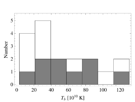
Figure 3: Histogram of core brightness temperature, in units of $10^{10}K$ at 5 GHz (grey) and 8.4 GHz (white) for 9 sources (0642+449 excluded).

The median core brightness temperature at 5 GHz is $5.6\times 10^{11}$ K, while at 8.4 GHz, the median value is slightly smaller at $3.2\times 10^{11}$ K. This can also be seen from a histogram of the core brightness temperature (Figure 3) where the 8.4 GHz values populate a larger majority of the lower bins. This may be as a result of the 8.4 GHz data probing regions of the jet where the physical conditions are intrinsically different, leading to lower observed brightness temperatures, similar to the results of Lee et al. (2008) at 86 GHz. However, it is difficult to separate this effect from any bias due to the resolution difference between 5 and 8.4 GHz. Furthermore, due to the relatively small difference between the median values, a larger sample size would be required to determine whether this is a real effect or just scatter in the data for the small number of sources observed here.

The maximum core brightness temperature at 5 GHz is $4.2\times 10^{12}$ K found in 0642+449 and the minimum value is $3.7\times 10^{10}$ K found in 2048+312. At 8.4 GHz, the maximum and minimum values are $7.3\times 10^{12}$ K (0642+449) and $7.4\times 10^{10}$ K (0636+680). Assuming that the intrinsic brightness temperature does not exceed the equipartition upper limit of $T_{eq}\sim 10^{11}$ K (Readhead, 1994), we can consider the observed core brightness temperatures in excess of this value to be the result of Doppler boosting of the approaching jet emission. Using the equipartition jet model of Blandford & Königl (1979) for the unresolved core region, we can estimate the Doppler factor ($\delta$) required to match the observed brightness temperatures ($T_{\rm b,obs}\sim 3\times 10^{11}\delta^{5/6}$). In most cases the Doppler factors required are modest, with values ranging from 1 to 5, except for 0642+449 which requires a Doppler factor of 23 at 5 GHz and 46 at 8.4 GHz.

From the observed brightness temperatures of the individual jets components, we can investigate the assumption of adiabatic expansion following Marscher (1990), Lobanov et al. (2001) and Pushkarev et al. (2008), who model the individual jet components as independent relativistic shocks with adiabatic energy losses dominating the radio emission. Note that this description of the outer jet differs from the $N\propto r^{-2}$, $B\propto r^{-1}$ case describing the compact inner jet region, which is not adiabatic. With a power-law energy distribution of $N(E)\propto E^{2\alpha-1}$ and a magnetic field described by $B\propto d^{-a}$, where $d$ is the transverse size of the jet and $a=1$ or $2$ corresponds to a transverse or longitudinal magnetic field orientation, we obtain

$$T_{\rm b,\,jet}=T_{\rm b,\,core}\left(\frac{d_{\rm core}}{d_{\rm jet}}\right)^{a+1-\alpha(a+4/3)}$$ (3)

which holds for a constant or weakly varying Doppler factor along the jet. Hence, we can compare the expected jet brightness temperature ($T_{\rm b,\,jet}$) with our observed values by using the observed core brightness temperature ($T_{\rm b,\,core}$) along with the measured size of the core and jet components ($d_{\rm core}$ and $d_{\rm jet}$) for a particular jet spectral index. We apply this model to the sources with extended jet structures to see if this model is an accurate approximation of the jet emission and also as a diagnostic of regions where the physical properties along the jet may change.

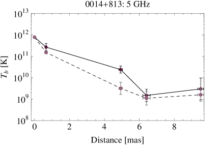
Figure 4: Brightness temperature ($T_{b}$) for components along the jet of 0014+813 at 5 GHz. The points connected by the dashed line represent the observed brightness temperatures while the points connected by the solid line represent the model values.

Figure 4 shows the comparison of this model (solid line) with the observed brightness temperatures (dashed line) along the jet of 0014+813 at 5 GHz. From the spectral index distribution obtained between 5 and 8.4 GHz, we adopt a jet spectral index of $\alpha=-1.0$ and assume a transverse magnetic field orientation ($a=1$) from inspection of the jet EVPAs (Fig. 2).The two jet components furthest from the core agree relatively well with the model, however, the two jet components closest to the core are substantially weaker than expected. Given the high RM for this source, it is also possible that the intrinsic magnetic field orientation is longitudinal; using a value of $a=2$ yields model brightness temperatures for these components that are within our measurement errors. Unfortunately, the extended jet emission at 8.4 GHz is not detected so we cannot constrain the jet RM and we also cannot rule out a change in the Doppler factor along the jet due to either an intrinsic change in the jet dynamics or a change in the jet direction. Clearly there are not enough observational constraints for this source to convincingly test the applicability of this model.

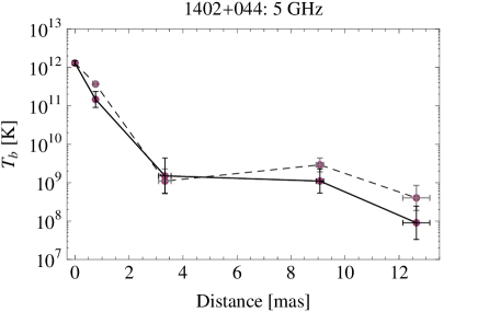
(a) 5 GHz data. Dashed line: observed; Solid line: model prediction with $\alpha=-0.5$.

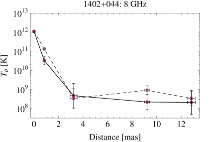
(b) 8.4 GHz data. Dashed line: observed; Solid line: model prediction with $\alpha=-0.5$.

Figure 5: Brightness temperature ($T_{b}$) for components along the jet of 1402+044 for both 5 and 8.4 GHz. The points connected by the dashed line represent the observed brightness temperatures while the points connected by the solid line represent the model values.

The observed brightness temperatures in the jet of 1402+044 at both 5 and 8.4 GHz (Figure 5) are in reasonable agreement with the model predictions for $\alpha=-0.5$, which is consistent with the overall jet spectral index distribution. Since the EVPA orientation implies a transverse magnetic field (Figure 2), we use $B\propto d^{-1}$. The jet components at 1 mas and 9 mas from the core both have observed brightness temperatures slightly higher than would be expected for radio emission dominated by adiabatic losses. Using flatter spectral index values of $\alpha=0.0$ and $\alpha=-0.3$, respectively, for these two components brings the model brightness temperatures within the measurement errors. Hence, it is likely that these components are subject to strong reacceleration mechanism that temporarily overcomes the energy losses due to the expansion of the jet.

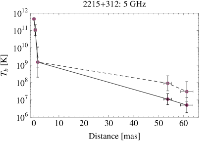
Figure 6: Brightness temperature ($T_{b}$) for components along the jet of 2215+312 at 5 GHz. The points connected by the dashed line represent the observed brightness temperatures while the points connected by the solid line represent the model values.

Applying the analysis to the jet of 2215+020 at 5 GHz (Figure 6), we see that the model matches the observed values very well for the two inner jet components using our measured spectral index of $\alpha=-0.7$ and a transverse magnetic field ($a=1$). However, the extended components brightness temperatures at 50–60 mas from the core are higher than expected by the adiabatic expansion model. This suggests different physical conditions in this region of the jet creating a less steep spectral index (using $\alpha=-0.5$ brings the model in line with the observed values). This far from the core it is likely that the Doppler factor has changed with either a change in the jet viewing angle or speed, possibly from interaction with the external medium. This is consistent with the observed strong brightening of the jet along with its change in direction from East to North-East, shown in Figure 2. Our results are very similar to those of Lobanov et al. (2001) who employed the same model for this source at 1.6 GHz.

4.2 Jet Structure and Environment

The added value of polarization observations in providing information on the compact inner jet structure is clear from the images of 1402+044 (Figure 2), 1557+032 (Figure 2) and 1614+051 (Figure 2), where polarized components are resolved on scales smaller than obtained from the total intensity image alone. For 1402+044, a higher resolution VSOP image at 5 GHz (Yang et al., 2008) resolved three components in the compact inner jet region consistent with what we find from the polarization structure of our lower resolution images where only one total intensity component is visible. In the case of 1557+032 and 1614+051, the identification of multiple polarized components in the core region, where again only one total intensity component is directly observed, suggests that observations at higher frequencies and/or longer baselines provided by, for example, the VSOP-2 mission (Tsuboi, 2009) are likely to resolve the total intensity structure of the core region. Hence, the polarization information is crucial in identifying the true radio core and helping to determine whether it corresponds to the $\tau=1$ frequency-dependent surface first proposed by Blandford & Königl (1979) or a stationary feature such as a conical shock (Cawthorne, 2006; Marscher, 2009) for a particular source.

For the sources with extended jets, substantial jet bends are observed. This is not a surprise since as long as the observations imply relativistic jet motion close to the line of sight, small changes in the intrinsic jet direction will be strongly amplified by projection effects. For example, an observed right-angle bend could correspond to an intrinsic bend of only a few degrees (e.g., Cohen et al., 2007). In the case of 1351-018, the jet appears to bend through $\sim 130^{\circ}$ (Figure 2) from a South-Easterly inner jet direction to a North-Westerly extended jet direction (see also Frey et al., 2002). The polarization distribution in the core region also supports an South-Easterly inner jet direction. This may be due to a helical jet motion along the line-of-sight as proposed, for example, for the jet of 1156+295 by Hong et al. (2004) or small intrinsic bends due to shocks or interactions with the external medium amplified by projection effects in a highly beamed relativistic jet (e.g., Homan et al., 2002). The jet bend at $\sim 400$ pc from the core of 2215+020 at 5 GHz may be due to a shock that also causes particle reacceleration, increasing the observed jet emission.

The core degree of polarization found in these sources is generally in the range 1–3%. Given that the emitted frequencies are in the range 20–45 GHz, we can compare these values to the core degrees of polarization observed in low-redshift AGN jets at 22 and 43 GHz (O’Sullivan & Gabuzda, 2009). In general, the core degree of polarization is higher in the low-redshift objects with values typically in the range 3–7%. This could be due to intrinsically more ordered jet magnetic field structures at lower redshifts or more likely, selection effects, since the AGN in O’Sullivan & Gabuzda (2009) were selected on the basis of known rich polarization structure while the high-redshift quasars had unknown polarization properties on VLBI scales. Another likely possibility is that the effect of beam depolarization (different polarized regions adding incoherently within the observing beam) is significantly reducing the observed polarization at 5 and 8.4 GHz due to our much larger observing beam compared with the VLBA at 22 and 43 GHz (factor of $\sim$3 better resolution even considering the longer baselines in the global VLBI observations).

Due to the extremely high redshifts, an observed RM of 50 rad m^-2 at $z\sim 3.5$ (average redshift for the sources in our sample) is equivalent to a nearby source with an RM of 1000 rad m^-2. The mean core $|$RM${}_{\rm min}^{\rm intr}|$ for our sample is $5580\pm 3390$ rad m^-2. Naively comparing our results with the 8–15 GHz sample of 40 AGN reported in Zavala & Taylor (2003, 2004), which has a median intrinsic core RM of $\sim 400$ rad m^-2 (and a median redshift of 0.7), suggests that the VLBI core RMs are higher in the early universe. However, RMs of the order of $10^{4}$ rad m^-2 have been measured in low to medium redshift sources at similar emitted frequencies (e.g., Attridge et al., 2005; Algaba et al., 2010); while some of the largest jet RM estimates, of order $10^{5}$ rad m^-2, have come through observation from 43–300 GHz of sources with redshifts ranging from $\sim 0.1$–2 (Jorstad et al., 2007). Furthermore, 15–43 GHz RM measurements of BL Lac objects from Gabuzda et al. (2006) and O’Sullivan & Gabuzda (2009) have a median intrinsic RM of $\sim 3000$ rad m^-2 and a median redshift of 0.34. Hence, from the small sample of minimum RM values presented in this paper it is not clear whether these sources are located in intrinsically denser environments or if the large RMs are simply due to the fact that the higher emitted frequencies are probing further upstream in the jet where it is expected that the electron density is higher and/or the magnetic field is stronger.

Our results from 5 to 8.4 GHz generally show flat to slightly steep core spectral indices with a median value of $\alpha=-0.3$. However, there is a large range of values going from $0.7$ for 0642+449 to $-1.0$ in the case of 1614+051. In the majority of cases, we find steep jet spectral indices ranging from $\alpha\sim-0.5$ to $-1.5$ with a median value of $\alpha=-1.0$. High-redshift objects are often searched for through their steep spectral index due to the relatively higher emitted frequencies for a particular observing frequency. The $z$–$\alpha$ correlation, as it is known, (i.e., steeper $\alpha$ at higher $z$) has been very successful (e.g., Broderick et al., 2007, and references therein) in finding high-redshift radio galaxies. While steeper spectral index values are expected simply from the higher rest frame emitted frequencies, Klamer et al. (2006) show that this cannot completely explain the correlation. The possible physical explanation they present is that the sources with the steepest spectral index values are located in dense environments where the radio source is pressure confined and hence, loses its energy more slowly. This effect might also apply to the dense nuclear environments of our sample of quasar jets. To test this we have plotted the core spectral index versus $|$RM${}_{\rm min}^{\rm intr}|$ in Figure 7. The data suggest that this is a useful avenue of investigation with a Spearman Rank test giving a correlation coefficient of -0.95, but clearly more data points are needed to determine whether there truly is a correlation or not.

Further observations of these sources with much better frequency coverage is required to properly constrain the spectral and RM distributions and to make detailed comparisons with low redshift sources to further investigate the quasar environment through cosmic time.

5 Conclusion

We have successfully observed and imaged 10 high-redshift quasars in full polarization at both 5 and 8.4 GHz using global VLBI. Model fitting two-dimensional Gaussian components to the total intensity data enabled estimation of the brightness temperature in the core and out along the jet. The observed high core brightness temperatures are consistent with modestly Doppler-boosted emission from a relativistic jet orientated relatively close to our line-of-sight. This can also explain the dramatic jet bends observed for some of our sources.

The core degrees of polarization are somewhat lower than observed from nearby AGN jets at similar emitted frequencies. However, beam depolarization is likely to have a stronger effect on these sources compared to the higher resolution observations of nearby sources. Model-fitting the polarization data enabled estimation of the minimum RM for each component since obtaining the exact value of the RM requires observations at three or more frequencies. For sources in which we were able to remove the integrated (foreground) RM, we calculated the minimum intrinsic RM and found a mean core $|$RM${}_{\rm min}^{\rm intr}|$ of 5580 rad m^-2 for four quasars with values ranging from $-1249$ rad m^-2 to 9110 rad m^-2. We found relatively steep core and jet spectral index values with a median core spectral index of $-0.3$ and a median jet spectral index of $-1.0$. We note that the expectation of denser environments at higher redshifts leading to larger RMs can also lead to steeper spectral indices through strong pressure gradients (Klamer et al., 2006) and that this hypothesis is not inconsistent with our results.

Several of the sources presented in this paper are interesting candidates for follow-up multi-frequency observations to obtain more accurate spectral and RM information in order to make more conclusive statements about the environment of quasar jets in the early universe and to determine whether or not it is significantly different to similar lower redshift objects.

Figure 1: Example plot of the uv coverage obtained for a representative source, 2048+312 at 5 GHz.

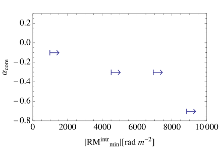
Figure 7: Plot of the intrinsic minimum RM (RM${}_{\rm min}^{\rm intr}$) versus the core spectral index between 5 and 8.4 GHz for each source. A Spearman Rank test gives a correlation coefficient of -0.95. However, more data points are required to determine whether there is a correlation or not.

References

- Algaba et al. (2010) Algaba J. C., Gabuzda D. C., Smith P. S., 2010, MNRAS, 411, 85
- Attridge et al. (2005) Attridge J. M., Wardle J. F. C., Homan D. C., 2005, ApJ, 633, L85
- Barthel et al. (1990) Barthel P. D., Tytler D. R., Thomson B., 1990, A&AS, 82, 339
- Bezrukovs & Gabuzda (2006) Bezrukovs V., Gabuzda D., 2006, in Proceedings of the 8th European VLBI Network Symposium
- Blandford & Königl (1979) Blandford R. D., Königl A., 1979, ApJ, 232, 34
- Broderick et al. (2007) Broderick J. W., Bryant J. J., Hunstead R. W., Sadler E. M., Murphy T., 2007, MNRAS, 381, 341
- Cawthorne (2006) Cawthorne T. V., 2006, MNRAS, 367, 851
- Cawthorne et al. (1993) Cawthorne T. V., Wardle J. F. C., Roberts D. H., Gabuzda D. C., Brown L. F., 1993, ApJ, 416, 496
- Cheung (2004) Cheung C. C., 2004, ApJ, 600, L23
- Cohen et al. (2007) Cohen M. H., Lister M. L., Homan D. C., Kadler M., Kellermann K. I., Kovalev Y. Y., Vermeulen R. C., 2007, ApJ, 658, 232
- Drinkwater et al. (1997) Drinkwater M. J., Webster R. L., Francis P. J., Condon J. J., Ellison S. L., Jauncey D. L., Lovell J., Peterson B. A., Savage A., 1997, MNRAS, 284, 85
- Fey & Charlot (1997) Fey A. L., Charlot P., 1997, ApJS, 111, 95
- Fey & Charlot (2000) Fey A. L., Charlot P., 2000, ApJS, 128, 17
- Fomalont (1999) Fomalont E. B., 1999, in G. B. Taylor, C. L. Carilli, & R. A. Perley ed., Synthesis Imaging in Radio Astronomy II Vol. 180 of ASPC Series, Image Analysis. p. 301
- Frey et al. (1997) Frey S., Gurvits L. I., Kellermann K. I., Schilizzi R. T., Pauliny-Toth I. I. K., 1997, A&A, 325, 511
- Frey et al. (2002) Frey S., Gurvits L. I., Lobanov A. P., Schilizzi R. T., Kawaguchi N., Gabányi K., 2002, in E. Ros, R. W. Porcas, A. P. Lobanov, & J. A. Zensus ed., Proceedings of the 6th EVN Symposium p. 89
- Frey et al. (2008) Frey S., Gurvits L. I., Paragi Z., É. Gabányi K., 2008, A&A, 484, 39
- Gabuzda (1999) Gabuzda D. C., 1999, New Astron. Rev., 43, 691
- Gabuzda et al. (2006) Gabuzda D. C., Rastorgueva E. A., Smith P. S., O’Sullivan S. P., 2006, MNRAS, 369, 1596
- Gabuzda et al. (1989) Gabuzda D. C., Wardle J. F. C., Roberts D. H., 1989, ApJ, 338, 743
- Ghisellini et al. (2009) Ghisellini G., Foschini L., Volonteri M., Ghirlanda G., Haardt F., Burlon D., Tavecchio F., 2009, MNRAS
- Gurvits et al. (2000) Gurvits L. I., Frey S., Schilizzi R. T., Kellermann K. I., Lobanov A. P., Kawaguchi N., Kobayashi H., Murata Y., Hirabayashi H., Pauliny-Toth I. I. K., 2000, Advances in Space Research, 26, 719
- Gurvits et al. (1992) Gurvits L. I., Kardashev N. S., Popov M. V., Schilizzi R. T., Barthel P. D., Pauliny-Toth I. I. K., Kellermann K. I., 1992, A&A, 260, 82
- Gurvits et al. (1994) Gurvits L. I., Schilizzi R. T., Barthel P. D., Kardashev N. S., Kellermann K. I., Lobanov A. P., Pauliny-Toth I. I. K., Popov M. V., 1994, A&A, 291, 737
- Gurvits et al. (1997) Gurvits L. I., Schilizzi R. T., Miley G. K., Peck A., Bremer M. N., Roettgering H., van Breugel W., 1997, A&A, 318, 11
- Hirabayashi et al. (1998) Hirabayashi H., Hirosawa H., Kobayashi H., Murata Y., Edwards P. G., Fomalont E. B., Fujisawa K., Ichikawa T., Kii T., Lovell J. E. J., the VSOP Collaboration. 1998, Science, 281, 1825
- Hogg (1999) Hogg D. W., 1999, arXiv:astro-ph/9905116
- Homan et al. (2002) Homan D. C., Wardle J. F. C., Cheung C. C., Roberts D. H., Attridge J. M., 2002, ApJ, 580, 742
- Hong et al. (2004) Hong X. Y., Jiang D. R., Gurvits L. I., Garrett M. A., Garrington S. T., Schilizzi R. T., Nan R. D., Hirabayashi H., Wang W. H., Nicolson G. D., 2004, A&A, 417, 887
- Hook et al. (1995) Hook I. M., McMahon R. G., Patnaik A. R., Browne I. W. A., Wilkinson P. N., Irwin M. J., Hazard C., 1995, MNRAS, 273, 63
- Jorstad et al. (2007) Jorstad S. G., Marscher A. P., Stevens J. A., Smith P. S., Forster J. R., Gear W. K., Cawthorne T. V., Lister M. L., Stirling A. M., Gómez J. L., Greaves J. S., Robson E. I., 2007, AJ, 134, 799
- Kaspi et al. (2007) Kaspi S., Brandt W. N., Maoz D., Netzer H., Schneider D. P., Shemmer O., 2007, ApJ, 659, 997
- Klamer et al. (2006) Klamer I. J., Ekers R. D., Bryant J. J., Hunstead R. W., Sadler E. M., De Breuck C., 2006, MNRAS, 371, 852
- Kudryavtseva et al. (2010) Kudryavtseva N., Britzen S., Witzel A., Ros E., Karouzos M., Aller M. F., Aller H. D., Terasranta H., Eckart A., Zensus A. J., 2010, arXiv1007.0989K
- Kuehr et al. (1983) Kuehr H., Liebert J. W., Strittmatter P. A., Schmidt G. D., Mackay C., 1983, ApJ, 275, L33
- Kuehr et al. (1981) Kuehr H., Witzel A., Pauliny-Toth I. I. K., Nauber U., 1981, A&AS, 45, 367
- Lee et al. (2008) Lee S., Lobanov A. P., Krichbaum T. P., Witzel A., Zensus A., Bremer M., Greve A., Grewing M., 2008, AJ, 136, 159
- Lister et al. (2009) Lister M. L., Cohen M. H., Homan D. C., Kadler M., Kellermann K. I., Kovalev Y. Y., Ros E., Savolainen T., Zensus J. A., 2009, AJ, 138, 1874
- Lobanov (2005) Lobanov A. P., 2005, arXiv:astro-ph/0503225
- Lobanov et al. (2001) Lobanov A. P., Gurvits L. I., Frey S., Schilizzi R. T., Kawaguchi N., Pauliny-Toth I. I. K., 2001, ApJ, 547, 714
- Marscher (1990) Marscher A. P., 1990, in J. A. Zensus & T. J. Pearson ed., Parsec-scale radio jets Interpretation of Compact Jet Observations. p. 236
- Marscher (2009) Marscher A. P., 2009, in Hagiwara Y., Fomalont E., Tsuboi M., Murata Y., eds, Approaching Micro-Arcsecond Resolution with VSOP-2: Astrophysics and Technology. Vol. 402. ASP Conf. Ser., San Francisco., p. 194
- McMahon et al. (1994) McMahon R. G., Omont A., Bergeron J., Kreysa E., Haslam C. G. T., 1994, MNRAS, 267, 9
- O’Dea (1990) O’Dea C. P., 1990, MNRAS, 245, 20
- Oren & Wolfe (1995) Oren A. L., Wolfe A. M., 1995, ApJ, 445, 624
- Osmer et al. (1994) Osmer P. S., Porter A. C., Green R. F., 1994, ApJ, 436, 678
- O’Sullivan & Gabuzda (2009) O’Sullivan S. P., Gabuzda D. C., 2009, MNRAS, 400, 26
- O’Sullivan & Gabuzda (2009) O’Sullivan S. P., Gabuzda D. C., 2009, MNRAS, 393, 429
- Paragi et al. (1999) Paragi Z., Frey S., Gurvits L. I., Kellermann K. I., Schilizzi R. T., McMahon R. G., Hook I. M., Pauliny-Toth I. I. K., 1999, A&A, 344, 51
- Piner et al. (2007) Piner B. G., Mahmud M., Fey A. L., Gospodinova K., 2007, AJ, 133, 2357
- Pushkarev et al. (2008) Pushkarev A., Kovalev Y., Lobanov A., 2008, in The role of VLBI in the Golden Age for Radio Astronomy http://pos.sissa.it/cgi-bin/reader/conf.cgi?confid=72, p.103
- Readhead (1994) Readhead A. C. S., 1994, ApJ, 426, 51
- Roberts et al. (1987) Roberts D. H., Gabuzda D. C., Wardle J. F. C., 1987, ApJ, 323, 536
- Shepherd (1997) Shepherd M. C., 1997, in G. Hunt & H. Payne ed., Astronomical Data Analysis Software and Systems VI Vol. 125 of ASPC Series, Difmap: an Interactive Program for Synthesis Imaging. p. 77
- Siemiginowska et al. (2003) Siemiginowska A., Smith R. K., Aldcroft T. L., Schwartz D. A., Paerels F., Petric A. O., 2003, ApJ, 598, 15
- Simard-Normandin et al. (1981) Simard-Normandin M., Kronberg P. P., Button S., 1981, ApJS, 45, 97
- Taylor et al. (2009) Taylor A. R., Stil J. M., Sunstrum C., 2009, ApJ, 702, 1230
- Tsuboi (2009) Tsuboi M., 2009, in Y. Hagiwara, E. Fomalont, M. Tsuboi, & M. Yasuhiro ed., Approaching Micro-Arcsecond Resolution with VSOP-2: Astrophysics and Technology. ASP Conf. Series. p. 30
- Veres et al. (2010) Veres P., Frey S., Paragi Z., Gurvits L. I., 2010, A&A
- Veron-Cetty & Veron (1989) Veron-Cetty M., Veron P., 1989, A Catalogue of quasars and active nuclei. ESO Scientific Report, Garching: European Southern Observatory (ESO).
- Veron-Cetty & Veron (1993) Veron-Cetty M., Veron P., 1993, A&AS, 100, 521
- Volvach et al. (2000) Volvach A. E., Nesterov N. S., Mingaliev M. G., 2000, Kinematika i Fizika Nebesnykh Tel Supplement, 3, 21
- Volvach (2003) Volvach O., 2003, in Quasar Cores and Jets, 25th IAU GA, 23-24 July 2003, Sydney, Australia. Vol. 18
- Yang et al. (2008) Yang J., Gurvits L., Lobanov A., Frey S., Hong X., 2008, A&A, 489, 517
- Yuan et al. (2003) Yuan W., Fabian A. C., Celotti A., Jonker P. G., 2003, MNRAS, 346, L7
- Zavala & Taylor (2003) Zavala R. T., Taylor G. B., 2003, ApJ, 589, 126
- Zavala & Taylor (2004) Zavala R. T., Taylor G. B., 2004, ApJ, 612, 749