Quantum state transmission in a cavity array via two-photon exchange

Abstract

The dynamical behavior of a coupled cavity array is investigated when each cavity contains a three-level atom. For the uniform and staggered intercavity hopping, the whole system Hamiltonian can be analytically diagonalized in the subspace of single-atom excitation. The quantum state transfer along the cavities is analyzed in detail for distinct regimes of parameters, and some interesting phenomena including binary transmission, selective localization of the excitation population are revealed. We demonstrate that the uniform coupling is more suitable for the quantum state transfer. It is shown that the initial state of polariton located in the first cavity is crucial to the transmission fidelity, and the local entanglement depresses the state transfer probability. Exploiting the metastable state, the distance of the quantum state transfer can be much longer than that of Jaynes-Cummings-Hubbard model. A higher transmission probability and longer distance can be achieved by employing a class of initial encodings and final decodings.

PACS number: 42.50.Pq, 05.60.Gg, 03.67.Hk

I INTRODUCTION

It is an important task in quantum information processing when a quantum state is transferred from one location to another. It refers to not only quantum communication zeilinger , but also large-scale quantum computing lloyd . Different protocols are proposed to realize quantum state transfer (QST). For example, based on measurement and reconstruction, an unknown quantum state can be faithfully transferred to an arbitrarily distant location via quantum teleportation ben . During the quantum teleportation, the measured result instead of the quantum state is transferred by a classical communication channel. Alternatively, a quantum state can be sent through a channel directly. There are two types of such state transfer which depends on the transfer distance. For long distance communication, the information encoded in photons can be transferred by an optical fiber cirac97 ; boozer , which has been widely used in quantum communication and cryptography applications muller ; ursin . Compared with the long distance communication, a kind of short distance communication which can be used between adjacent quantum processors was recently introduced bose03 . Using an unmodulated spin chain as a channel, the state transmits from one end of the chain to another with some fidelity. Subsequently, many schemes are proposed to gain higher even perfect transfer fidelity chr ; chr05 ; ross09 ; linden2004 ; zou ; bish ; lukin11 .

On account of the possibility of individual addressing, an array of coupled cavities is probably a promising candidate for simulating spin chains. The coupled cavities can be realized in various physical systems kimble , such as photonic crystals hen , superconducting resonators scho , and cavity-fiber-cavity system sera . So far, the Heisenberg chains of spin $1/2$ har2007 , of any high spin cho , and with next-nearest-neighbor interactions chen are simulated in the coupled cavities. In these simulation processes, the cavity field is ingeniously removed, and the same procedure occurs when the QST is investigated in Ref. li09 . However, the array of coupled cavities, a hybrid system combining the spinor atom and photons, would provide richer phenomena than the pure spin chains or Bose-Hubbard model hartmann2006 ; greentre2006 ; mak2008 . For this reason, the temporal dynamics kim08 ; mak ; ciccarello and the binary transmission zhang10 ; yang11 , i.e., the QST including both components in one-dimensional (1D) coupled cavities, are analyzed in detail.

The binary transmission mentioned above is restricted in single-excitation subspace, i.e., only one photon transfers along the cavities in cascades, and usually the transfer distant extensively depends on the lifetime of atomic excitation state. Quite recently, the two-photon propagation in waveguide has been attracting increasing interest from many researchers, such as two-photon transport in 1D waveguide coupled to a two-level emitter fan07 , a three-level emitter roy , and a nonlinear cavity law . Compared with one-photon electric-dipole E1 transition, the two-photon 2E1 transition that emits two photons simultaneously is a second-order transition mokler . Therefore, the metastable state decaying via 2E1 transition has remarkable longer lifetime than the excited state decaying via E1 transition. The typical example is the lifetime for the $2^{2}S_{1/2}$ state in hydrogen is of the order of fractions of a second, which is several orders longer than that of single-photon excitation state. The long lifetime of the metastable state could provide sufficient operation time to transfer information. More recently, Law et al. reveal that the photons trend to bound together law2011 in the two-excitation subspace when the ratio of vacuum Rabi frequency to the tunneling rate between cavities exceeds a critical value. Motivated by these aspects, it is desired to explore the short distance binary transmission of the model that bounding two photons as a quasiparticle alex2010 ; alex .

In this work, we investigate the binary transmission in 1D array of coupled cavities, each of which contains a three-level atom. By adiabatically eliminating the intermediate state, the individual cavity can be described by the two-photon Jaynes-Cummings (JC) model with a metastable state and a ground state. In the single-atom excitation subspace, the system Hamiltonian is able to be diagonalized exactly. It allows us to focus on the binary transmission with the explicit expression of the excitation population. We consider the uniform and staggered intercavity hopping in different parameters regimes, especially in the strong coupling and strong hopping limits. With the uniform hopping, we find that the initial state of polariton located in the first cavity is essential to the transmission fidelity. When the polariton is a pure atomic state, an oscillation behavior in the envelopment of fidelity occurs and the state transfer probability increases obviously. On resonance, we reveal the optimal transmission time is mainly governed by the intercavity hopping strength and the system size. We also show that the exploiting of the metastable state overcomes the deficit of short transfer distance during the lifetime of excitation state mak . With the staggered hopping, the excitation population trends to be localized in the first several cavities and slows down the transfer speed. This phenomenon becomes more distinct as the distortion of the hopping strength enlarges. In the free evolution of the system, the transmission fidelity drops quickly as the size of the array increases. How to enhance the fidelity of the transmission is important, since the fidelity of QST is expected to be better than that by using straightforward classical communication. We finally demonstrate that a class of initial encoding and final decoding process, which is currently used in spin chains zou ; bish , can also greatly improve the performance of binary transmission.

The paper is organized as follows. In Sec. II, we discuss the dynamics of an array of coupled cavities with the uniform coupling. In Sec. III, we consider the general situation with staggered coupling between the adjacent cavities. Section IV gives an effective method to improve the fidelity of the quantum state transfer by encoding and decoding limited qubits in strong coupling regime. In Sec. V, we give a brief conclusion to the paper.

II THEORY MODEL

We consider an array of coupled cavities, each of which contains a three-level atom in cascade configuration. The individual cavity is tuned to two-photon resonance with the metastable state $\left|e\right\rangle$ and the ground state $\left|g\right\rangle$, and these two states are coupled to an intermediate state $\left|i\right\rangle$ with a single mode of the electromagnetic field with coupling strengths $g_{1}$ and $g_{2}$ respectively. The intermediate level is detuned by the amount $\delta$ from the average of the energies of the $\left|e\right\rangle$ and $\left|g\right\rangle$. In the large detuning condition $|\delta|>>g_{1},g_{2}$, the intermediate state can be adiabatically eliminated, and the Hamiltonian of one individual cavity can be written as a two-photon JC model buzek ; alex1998 (here $\hbar=1$)

$$\mathcal{H}^{(i)}=\omega_{a}\sigma_{ee}^{(i)}+\omega_{c}a_{i}^{\dagger}a_{i}+\lambda\left(\sigma_{eg}^{(i)}a_{i}^{2}+\sigma_{ge}^{(i)}a_{i}^{\dagger 2}\right),$$ (1)

where $a_{i}$ ($a_{i}^{\dagger}$) is the photonic annihilation (creation) operator, and $\sigma_{ge}^{(i)}=\left|g\right\rangle^{(i)(i)}\left\langle e\right|$ ($\sigma_{eg}^{(i)}=\left|e\right\rangle^{(i)(i)}\left\langle g\right|$) is atomic transition operator in the $i$th cavity, $\omega_{c}$ is the resonance frequency of the cavity and $\omega_{a}$ is the effective energy of atom. The metastable state $\left|e\right\rangle$ and the ground state $\left|g\right\rangle$ is coupled by a two-photon process with strength $\lambda$, which is given as $\lambda=g_{1}g_{2}/\delta$. The two-photon JC model has been experimentally realized in high-Q superconducting microwave cavity brune1987 .

In Hamiltonian (1), the operator $Q^{(i)}=a_{i}^{\dagger}a_{i}+$ $\sigma_{ee}^{(i)}-\sigma_{gg}^{(i)}$ commutes with $\mathcal{H}^{(i)}$, implying that the total number of atomic inversion and photonic excitation is conserved. The two-photon JC Hamiltonian can be diagonalized analytically. Spanned by the subspace $\left\{\left|e,n-2\right\rangle^{(i)},\left|g,n\right\rangle^{(i)}\right\}$ ($n$ $\geq$ $2$), where $n$ is the number of photons, the Hamiltonian can be written by the polaritonic state as

$$\mathcal{H}_{n}^{(i)}=\left(\begin{array}[]{cc}\omega_{a}+n\omega_{c}-2\omega_{c}&\lambda\sqrt{n\left(n-1\right)}\\ \lambda\sqrt{n\left(n-1\right)}&n\omega_{c}\end{array}\right).$$ (2)

The eigenvalues and eigenfunctions of $\mathcal{H}_{n}^{(i)}$ can be written in terms of the dressed-state representation

$$\left|\pm,n\right\rangle^{(i)} = \chi^{\pm}(\theta_{n})\left|g,n\right\rangle^{(i)}\pm\chi^{\mp}(\theta_{n})\left|e,n-2\right\rangle^{(i)},$$ (3)

$$E_{\pm,n}^{(i)} = \frac{\Delta}{2}+n\omega_{c}\pm 2\chi_{n},\quad\left(n\geqslant 2\right)$$ (4)

where $\tan\theta_{n}={2\lambda\sqrt{n(1+n)}}/(\Delta+2\chi_{n})$, $\chi^{+}\left(x\right)=\sin x$, $\chi^{-}\left(x\right)=\cos x$, $\chi_{n}=\sqrt{n(n-1)\lambda^{2}+\Delta^{2}/4}$, and the detuning $\Delta=\omega_{a}-2\omega_{c}$.

The $N$ cavities linked via two-photon exchange are described by the Hamiltonian

$$\mathcal{H}=\sum\limits_{i=1}^{N}\mathcal{H}^{(i)}+\xi\sum\limits_{i,j=1}^{N}A_{ij}\left(a_{i}^{\dagger 2}a_{j}^{2}+a_{i}^{2}a_{j}^{\dagger 2}\right),$$ (5)

where $\xi$ is the intercavity coupling of double photons and $A$ is the adjacency matrix of the connectivity graph. Here the photons only hop between the nearest-neighbor cavities, so the matrix element is given by $A_{ij}=\delta_{i,j\pm 1}$.

Since the hopping between cavities does not change the number of photons, the operator $Q=\sum\nolimits_{i}Q^{(i)}$ commutes with the Hamiltonian $\mathcal{H}$. For simplicity, the analysis is restricted to the case of $Q=2-N$, i.e., the system contains only single-atom excitation or two-photon excitation. Here it is assumed that all the cavities are equal. Then we extract the site indexes from the atomic and field operators, and define them as a set of bare bases which form a complete Hilbert space. The system bases thus can be written as $\left|M\right\rangle\otimes\left|g,2\right\rangle$ and $\left|M\right\rangle\otimes\left|e,0\right\rangle$ $(M=1,2,...,N)$, which denote that there are two photons or an atomic excitation at cavity $M$. In these restricted bases, the Hamiltonian (5) can be represented as

$$\mathcal{H}_{\mathrm{res}}=\frac{\Delta}{2}I_{N}\otimes Z+\sqrt{2}\lambda I_{N}\otimes X+2\xi A\otimes\frac{I_{2}-Z}{2},$$ (6)

where $I_{m}$ is the $m\times m$ identity matrix and $X$, $Z$ are the pauli operators acting on the certain site of cavity. If the open chain of the coupled cavity is considered, i.e., the hard-wall boundary conditions are assumed, the eigenvectors of the adjacency matrix $A$ are chr ; mak $\left|m\right\rangle=\sqrt{\frac{2}{N+1}}\sum\nolimits_{M}\sin\left(\frac{mM\pi}{N+1}\right)\left|M\right\rangle$, with corresponding eigenvalues $E_{m}=-2\cos\frac{m\pi}{N+1}$ for all $m=1,2,...,N$. For a 1D chain of cavities, the Hamiltonian $\mathcal{H}_{\mathrm{res}}$ can be expressed in the bases $\left\{\left|m\right\rangle\otimes\left|e,0\right\rangle,\left|m\right\rangle\otimes\left|g,2\right\rangle\right\}$ as block diagonal matrixes, in which the $m$th block appears as

$$\mathcal{H}_{\mathrm{res}}(m)=\left(\begin{array}[]{cc}\frac{\Delta}{2}&\sqrt{2}\lambda\\ \sqrt{2}\lambda&-\frac{\Delta}{2}-4\xi\cos\frac{m\pi}{N+1}\end{array}\right).$$ (7)

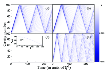
Figure 1: (Color online) The probability of the certain cavity as a function of time with the length of the chain $N=101$ and on resonance $\Delta=0$ for the initial state $\beta=\pi/4$. The upper two plots show the population of atom (a) and photon (b) in the strong J-C coupling regime ($\lambda=200\xi$), and the lower two plots are the population of atom (c) and photon (d) in the strong hopping regime ($\lambda=\xi/200$). The inset of (c) shows the population of the atom in the first cavity slowly decreases with time.

Then the block matrix can be diagonalized, the eigenvalues are $E_{\pm}^{m}=-2\xi\cos\left(\frac{m\pi}{N+1}\right)\pm\sqrt{\left[\frac{\Delta}{2}+2\xi\cos\left(\frac{m\pi}{N+1}\right)\right]^{2}+2\lambda^{2}}$, and the corresponding eigenvectors are $\left|m,\pm\right\rangle=\left|m\right\rangle\otimes\left|\pm\right\rangle$, where the dressed state $\left|\pm\right\rangle=[\left(\Delta-2E_{\mp}^{m}\right)\left|e,0\right\rangle+2\sqrt{2}\lambda\left|g,2\right\rangle]/\sqrt{\left(\Delta-2E_{\mp}^{m}\right)^{2}+8\lambda^{2}}$. With these analytical expressions, the time evolution of arbitrary $N$ cavities can be straightforwardly derived. In the following, the quantum state transfer is studied in such model. It should be emphasized that there exist two channels, either atomic or photonic, to transfer information, which is different from state transfer in a pure spin chain. In this model, the sender and receiver can select which qubit is encoded and decoded. The ground state of the system $\left|g,0\right\rangle^{\otimes N}$ with a zero eigenenergy will not involve any evolution by the Hamiltonian $\mathcal{H}$. So only the propagation of the excitation state for atom and photons needs to be considered.

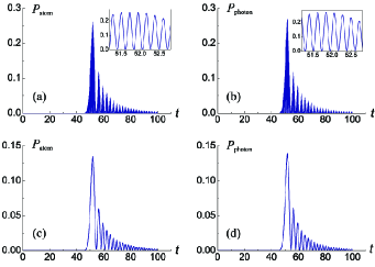
Figure 2: (Color online) Dynamics of the transfer probabilities of atom and photon respectively in strong coupling limit. The system parameters are $\ \Delta=0,\lambda=10,\xi=1,N=100$ for (a) and (b) $\beta=\pi/2$, (c) and (d) $\beta=\pi/4$. The insets of (a) and (b) show the oscillation behavior in the envelopment.

The influence of the initial state located in the first cavity is investigated. Supposing that the initial state is an entangled state in the first cavity

$$\left|\varphi(t=0)\right\rangle=\left|M=1\right\rangle\otimes\left(\cos\beta\left|g,2\right\rangle+\sin\beta\left|e,0\right\rangle\right),$$ (8)

the state at time $t$ is given by $\left|\varphi(t)\right\rangle=U(t)\left|\varphi(0)\right\rangle$, where $U(t)=e^{-i\mathcal{H}t}$ is the evolution operator of the whole system. Hence one has

$$\left|\varphi(t)\right\rangle=\sum\limits_{M,m=1}^{N}\left|M\right\rangle\otimes\left[f_{M,m}^{+}\left(t\right)\left|+\right\rangle+f_{M,m}^{-}\left(t\right)\left|-\right\rangle\right],$$ (9)

where the probability amplitudes are given by

$$f_{M,m}^{\pm}\left(t\right) = \frac{2}{N+1}e^{-iE_{\pm}^{m}t}\chi^{\pm}\left(\beta-\alpha_{m}\right)$$ (10)

$$\times\sin\left(\frac{m\pi}{N+1}\right)\sin\left(\frac{mM\pi}{N+1}\right),$$

with $\tan\alpha_{m}=-\{[\left(\Delta-2E_{+}^{m}\right)^{2}+8\lambda^{2}]/[\left(\Delta-2E_{-}^{m}\right)^{2}+8\lambda^{2}]\}^{1/2}$. Thus, the probabilities of occupation for atom and photons at the $s$th cavity are given by

$$P_{\mathrm{atom/photon,s}}=\left|\sum\limits_{m=1}^{N}\left[f_{s,m}^{\pm}\chi^{-}(\alpha_{m})\pm f_{s,m}^{\mp}\chi^{+}\left(\alpha_{m}\right)\right]\right|^{2}.$$ (11)

It is assumed that the system is on resonant condition, i.e., $\Delta=0$. If the coupling in each cavity dominates the evolution, i.e., in the so called strong coupling limit $\lambda>>\xi$, the Hamiltonian becomes$\ \mathcal{H}_{\mathrm{res}}=\xi A\otimes I_{2}$ which has ignored the fast-rotating terms in the interaction picture. Such Hamiltonian mimics two Heisenberg spin chains kay2008 in atomic and photonic channels respectively. Then the information transferred from sender to receiver can be encoded in either channel with speed $\xi$, and the selectivity of channels may be useful in binary communication. Compared with the Ref. mak , due to the bounding effect of photon discussed here, the time for the quantum state transfer is reduced by half given the both system have the same hopping strength (see Fig. 1 (a) and (b)). In other limit, that the hopping dominates the evolution, i.e., $\xi>>\lambda$, the Hamiltonian reduces to $\mathcal{H}_{\mathrm{res}}=2\xi A\otimes\left(I_{2}-Z\right)/2$. Governed by such Hamiltonian, only the photon is delocalized on the whole coupled cavity array with double speed $2\xi$ (Fig. 1 (d)), whereas the atomic population is trapped in the first cavity without dispersion (Fig. 1 (c) and the inset in it).

In the following of this section, we focus our interest on the binary transmission in the strong coupling limit. We find that the temporal evolution of the state vector sensitively depends on the initial state of the system. When $\beta=\pi/2$, i.e., the initial localized excitation is purely atomic, Figs. 2 (a) and (b) show that both probabilities oscillate in each envelopment and have the same transmission behavior. When $\beta=\pi/4$, the initial state is the maximum entangled state localized in the first cavity. Meanwhile $\alpha_{m}\simeq-\pi/4$ in the strong coupling limit on resonance. Then the transfer probabilities can be expressed simply as $P_{\mathrm{atom/photon,N}}\simeq 2\left|\sum\nolimits_{m}e^{-iE_{+}^{m}t}\sin\left(\frac{m\pi}{N+1}\right)\sin\left(\frac{mN\pi}{N+1}\right)\right|^{2}/\left(N+1\right)^{2}$. Figs. 2 (c) and (d) show that the evolution of system has a similar behavior as that of $\beta=\pi/2$. However, due to the coherence of the initial local state, the oscillation in each envelopment disappears. Furthermore, the maximum of transition probability is $0.135$ and $0.139$ for atom and photon at time $51.84$ and $51.73$ respectively, which are about half of those for $\beta=\pi/2$.

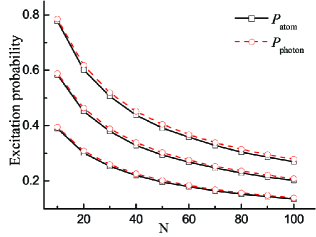
Figure 3: (Color online) The binary transmission probabilities verse the number of cavities with different $\beta$. From top to bottom, $\beta=0$, $\beta=\pi/6$, and $\beta=\pi/4$, with the system parameters are $\Delta=0$, $\lambda=10$, and $\xi=1$.

The maximum of transmission probabilities for various cavity lengths with different $\beta$ is numerically evaluated. Fig. 3 shows that the entangled state located in the first cavity does not provide any benefit to the transmission probability, and the transition probability of atomic channel is slightly less than that of photonic channel for various values of $\beta$. Also, the maximum transmission probabilities decrease with the number of cavities $N$.

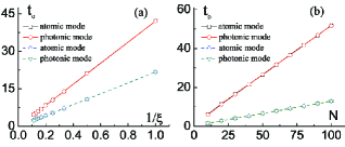
Figure 4: (Color online)   On resonance, the optimal time $t_{o}$ of binary transmission as a function of (a) $\xi$, from top to bottom, $N=80$ and $N=40$ with $\lambda=80$ and $\beta=0$; (b) $N$, from top to bottom, $\xi=1$ and $\lambda=10$, $\xi=4$ and $\lambda=40$ with $\beta=0$.

The binary-channel optimal time $t_{o}$ can be explored when the transmission probability achieves its maximum. It is found that the time $t_{o}$ is not sensitive to the cavity-atom coupling $\lambda$ in the strongly coupling limit, while it is highly dependent on the number of the cavities $N$ and intercavity hopping amplitude $\xi$. As shown in Fig. 4 (a), $t_{o}$ of atomic and photonic modes is plotted with respect to $1/\xi$ for $N=40$ and $N=80$ with $\lambda=80$ when two photons are initially located in the first cavity. The atomic optimal time is nearly identical to that of the photonic mode. A linear dependence of both $t_{o}$ on $1/\xi$ is depicted, and the ratio increases with respect to the length of the cavity array $N$, as is also confirmed in Fig. 4 (b). The farther the distance is, the more time the propagation needs. The time $t_{o}$ scales linearly with $N$ for atomic and photonic modes. Therefore, the optimal time satisfies $t_{o}\sim N/\xi$. Thus, the optimal time can be tuned by controlling intercavity hopping strength and system size.

Finally, we give a comparison between this scheme and that based on the Jaynes-Cummings-Hubbard model mak . We note that in contrast to single-photon JC coupling $g$ used in that model, the two-photon coupling strength $\lambda\simeq g^{2}/\delta\sim 0.1g$ (assuming $g_{1}=g_{2}=g$). To preserve the strong coupling condition, $\lambda=10\xi$ for instance, the speed of the quantum transfer will reduce to $2\xi\simeq 0.02g$ considering the photon’s bounding effect, which is about $1/5$ of that of the Jaynes-Cummings-Hubbard model. With the same parameters used in Figs. 2 (c) and (d), the maximum excitation probabilities of atom and field are $0.139$ and $0.141$ at time $10.41$ and $10.40$ mak . It is clear that the weakening of the transmission fidelity in our scheme is less than $0.01$, which is nearly neglectable. However, due to the long lifetime of metastable states, the distance of the propagation can obviously increase during the lifetime of atom. For instance, the spontaneous emission lifetimes of the $D_{5/2}$ metastable state and the $P_{1/2}$ level of ⁴⁰Ca⁺ ion trapped in high finesse optical cavity are about $1s$ blatt04 and $7ns$ buzek01 respectively, which leads to an increase of propagation distance with a seven order of magnitude when the metastable state is exploited in the scheme.

III STAGGERED HOPPING

Compared with the uniform hopping, a parabolic hopping was firstly advanced in theory to achieve the perfect quantum transfer, and the dynamic behavior of such kind of hopping is elaborately investigated in 1D Jaynes-Cummings-Hubbard model mak . Recently, there is another kind of hopping ciccarello called staggered hopping draws much interest. Some models with the staggered next-nearest coupling have been widely studied in condensed matter physics. For instance, a Peierls distorted chain pei can be used as a data bus huo08 to transfer the information. In this section, we consider the staggered pattern of hopping strengths, i.e., the hopping strength of the next-nearest cavities are different between odd-to-even and even-to-odd, which is controlled by the distortion of the hopping strength $\kappa$. To solve this model, we exploited the same process dealt with Eq. (5), which first diagonalize the auxiliary Hilbert space spanned by the site of the cavity $\{\left|M\right\rangle\}$. Here the matrix element of the adjacency matrix $A$ in $\mathcal{H}_{\mathrm{res}}$ is rewritten as $A_{ji}=A_{ij}=[1-\kappa(-1)^{i}]\delta_{i+1,j}$, $(i\leqslant j)$. Here, we assume that the number of the cavities is odd, and hence the numbers of strong bonds and weak bonds are equal. The eigenvectors of this adjacency matrix are given as

$$\left|o\right\rangle =\frac{2}{\kappa-1}\sqrt{\frac{\kappa}{\tau^{N+1}-1}}\sum\limits_{M=1}^{\frac{N+1}{2}}\tau^{M-1}\left|2M-1\right\rangle,$$ (12)

$$\left|m\right\rangle_{\pm} =\sqrt{\frac{2}{N+1}}\bigg{[}\sum\limits_{M=1}^{\frac{N-1}{2}}\sin\left(\frac{2mM\pi}{N+1}\right)\left|2M\right\rangle$$

$$\pm\sum\limits_{M=1}^{\frac{N+1}{2}}\sin\left(\frac{2mM\pi}{N+1}+\theta_{m}\right)\left|2M-1\right\rangle\bigg{]},\text{ }$$ (13)

with corresponding eigenvalues

$$\varepsilon_{o} = 0,$$ (14)

$$\varepsilon_{m_{+}} = -\varepsilon_{m_{-}}=2\sqrt{\cos^{2}\frac{m\pi}{N+1}+\kappa^{2}\sin^{2}\frac{m\pi}{N+1}},$$ (15)

where the bond alternation parameter $\tau=\frac{\kappa+1}{\kappa-1}$ and the angle $\theta_{m}$ satisfies

$$e^{i\theta_{m}}=\frac{1-\kappa}{\varepsilon_{m_{+}}}\left(e^{-i\frac{2m\pi}{N+1}}-\tau\right).\text{ }m=1,2,...,\frac{N-1}{2}$$ (16)

Now we investigate the dynamical behavior of the system under this staggered coupling. In the $\upsilon$th block, the Hamiltonian is given as

$$H_{\mathrm{res}}(\upsilon)=\left(\begin{array}[]{cc}\frac{\Delta}{2}&\sqrt{2}\lambda\\ \sqrt{2}\lambda&-\frac{\Delta}{2}+2\xi\varepsilon_{\upsilon}\end{array}\right),\text{ }\upsilon=o,m_{\pm}$$ (17)

The eigenvectors of the $\upsilon$th block of the Hamiltonian are

$$\left|\upsilon,\pm\right\rangle=\left|\upsilon\right\rangle\otimes\left|\pm_{\upsilon}\right\rangle=\left|\upsilon\right\rangle\otimes\frac{\left(\Delta-2E_{\mp}^{\upsilon}\right)\left|e,0\right\rangle+2\sqrt{2}\lambda\left|g,2\right\rangle}{\sqrt{\left(\Delta-2E_{\mp}^{\upsilon}\right)^{2}+8\lambda^{2}}},$$ (18)

with the corresponding eigenenergy

$$E_{\pm}^{\upsilon}=\xi\varepsilon_{\upsilon}\pm\sqrt{\left(\frac{\Delta}{2}-\xi\varepsilon_{\upsilon}\right)^{2}+2\lambda^{2}}.$$ (19)

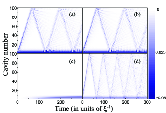
Figure 5: (Color online) The probability of the certain cavity as a function of time with the staggered coupling. The upper two plots show the population of atom (a) and photon (b) in the strong coupling regime ($\lambda=200\xi$), and the lower two plots are the population of atom (c) and photon (d) in the strong hopping regime ($\lambda=\xi/200$). The parameters are $\beta=\pi/4$, $\Delta=0$, $N=101$, $\kappa=-0.2$.

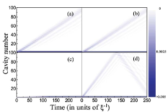
Figure 6: (Color online) The probability of the certain cavity as a function of time with the staggered coupling. The upper two plots show the population of atom (a) and photon (b) in the strong coupling regime ($\lambda=200\xi$), and the lower two plots are the population of atom (c) and photon (d) in the strong hopping regime ($\lambda=\xi/200$), with the system parameters are $\beta=\pi/4$, $\Delta=0$, $N=101$, and $\kappa=-0.8$.

For the initial entangled state Eq. (8) in the first cavity, the excitation populations of the atom and field in the $s$th cavity after time $t$ are

$$P_{\mathrm{atom,s}} = |\sum\limits_{\upsilon,m}c_{\upsilon}c_{\upsilon}^{\prime}[\chi^{-}\left(\alpha_{\upsilon}\right)\chi^{+}\left(\beta-\alpha_{\upsilon}\right)e^{-iE_{+}^{\upsilon}t}$$ (20)

$$+\chi^{+}(\alpha_{\upsilon})\chi^{-}\left(\beta-\alpha_{\upsilon}\right)e^{-iE_{-}^{\upsilon}t}]|^{2}.$$

$$P_{\mathrm{photon,s}} = |\sum\limits_{\upsilon,m}c_{\upsilon}c_{\upsilon}^{\prime}[-\chi^{+}(\alpha_{\upsilon})\chi^{+}\left(\beta-\alpha_{\upsilon}\right)e^{-iE_{+}^{\upsilon}t}$$ (21)

$$+\chi^{-}(\alpha_{\upsilon})\chi^{-}\left(\beta-\alpha_{\upsilon}\right)e^{-iE_{-}^{\upsilon}t}]|^{2},$$

where $\tan\alpha_{\upsilon}=-\{[\left(\Delta-2E_{+}^{\upsilon}\right)^{2}+8\lambda^{2}]/[\left(\Delta-2E_{-}^{\upsilon}\right)^{2}+8\lambda^{2}]\}^{1/2}$ and the amplitudes $c_{\upsilon}^{\prime}$ are dependent on the site of the cavity, when $s$ is odd

$$c_{o}^{\prime}=\frac{2}{\kappa-1}\sqrt{\frac{\kappa}{\tau^{N+1}-1}}\tau^{\frac{s-1}{2}},$$ (22)

$$c_{m_{+}}^{\prime}(m)=-c_{m_{-}}^{\prime}(m)=\sqrt{\frac{2}{N+1}}\sin\left[\frac{(s+1)m\pi}{N+1}+\theta_{m}\right],$$ (23)

and when $s$ is even

$$c_{o}^{\prime} = 0,$$ (24)

$$c_{m_{+}}^{\prime}(m) = c_{m_{-}}^{\prime}(m)=\sqrt{\frac{2}{N+1}}\sin\left(\frac{sm\pi}{N+1}\right).\text{ }$$ (25)

The amplitudes of the initial state $c_{\upsilon}$ equal to $c_{\upsilon}^{\prime}$ with $s=1$.

When the distortion $\kappa\rightarrow 0$, it returns to the uniform coupling discussed above. Here, the behavior of the system is studied in both strong coupling and hopping region for different values of $\kappa$. Figs. 5 (a) and (b) show the evolution of the excitation along the array in the strong coupling limit when $\kappa=-0.2$. Compare with the uniform case, the maximum of excitation probability reduces to $0.08$, and the speed of the propagation slows down lightly. When $\kappa=-0.8$, Figs. 6 (a) and (b) show that it further reduces the speed and considerably lessens the excitation probability, and the population is almost localized in the first cavity. In the strong hopping limit, Fig. 5 (c) shows the atomic population distributes on the first several cavities, especially the first several odd cavities, while the amplitude of the even sites vanishes. For the photonic mode, the speed is double referring to the strong coupling and the maximum of excitation probability also reaches $0.08$ (see Fig. 5 (d)). When the hopping dominates, as the distortion increases to $-0.8$, only the photon transfers along the array with the maximum excitation probability $0.0026$ (see Figs. 6 (c) and (d)).

IV MULTIQUBIT ENCODING

It is well known that the highest fidelity for classical transmission of a quantum state is $2/3$ horodecki . However, Fig. 3 implies that even in the case of $\beta=0$, the transmission fidelity exceeds $2/3$ in a very short distance. Therefore, the further improvement of the transfer probability of the state is necessary. In spin system, there are several methods to improve the fidelity of state transfer, such as modulating the couplings chr , or turning on/off the coupling on demand ross09 . Alternatively, one can improve the communication by encoding the information in the multiple spins linden2004 ; zou ; bish without engineering the coupling.

In Ref. mak , a Gaussian wave packet is exploited as the initial state. However, encoding all the qubits through the coupled cavity array is difficult to achieve in reality. Here, an alternative $k$-qubit encoding is used, which only needs limited number of qubits to be encoded and decoded by the sender and receiver. In Sec. III, we have shown that the excitation populations are almost trapped in the first several cavities either in strong coupling or strong hopping. So we will focus the quantum transfer in the uniform coupling discussed in Sec. II rather than the staggered hopping, especially in the strong coupling regime. If a $k$-qubit encoding is used as the initial state $\left|\varphi(t=0)\right\rangle_{k}=\sum\nolimits_{\nu=0}^{k-1}\left(-1\right)^{\nu}\left|M=2\nu+1\right\rangle\otimes\left|e,0\right\rangle/\sqrt{k}$, the maximum value can be achieved for $k=2$, which means that one cannot get a higher transmitting probability even using more qubits to encode. To obtain a higher transmitting probability, the decoding process at the another site of the cavities must be considered. The excitation state of the first cavity would ideally propagate to the $\left[N-2\left(r-1\right)\right]$th site of the cavities, while the excitation state of the last cavity of the encoding would ideally propagate to the $N$th site of the cavities, i.e., $\left|\varphi_{\mathrm{idea}}\right\rangle_{\mathrm{atom}}=\sum\nolimits_{q=0}^{r-1}\left(-1\right)^{q}\left|M=M_{q}\right\rangle\otimes\left|e,0\right\rangle/\sqrt{r}$ and $\left|\varphi_{\mathrm{idea}}\right\rangle_{\mathrm{photon}}=\sum\nolimits_{q=0}^{r-1}\left(-1\right)^{q}\left|M=M_{q}\right\rangle\otimes\left|g,2\right\rangle/\sqrt{r}$, where $M_{q}=N-2\left(r-1\right)+2q$. Thus the probabilities of excitation can be calculated as

$$P_{\mathrm{atom/photon}}=\left|\frac{1}{\sqrt{r}}\sum\limits_{m=1}^{N}\sum\limits_{q=0}^{r-1}\mu_{m,q}^{\pm}\right|^{2},$$

where $\mu_{m,q}^{\pm}=(-1)^{q}[\tilde{f}_{M_{q},m}^{\pm}\chi^{-}\left(\alpha_{m}\right)\pm\tilde{f}_{M_{q},m}^{\mp}\chi^{+}\left(\alpha_{m}\right)]$, with the probability amplitudes

$$\tilde{f}_{M,m}^{\pm}\left(t\right) = \frac{2}{\left(N+1\right)\sqrt{k}}\sum\limits_{\nu=0}^{k-1}\left(-1\right)^{\nu}e^{-iE_{\pm}^{m}t}\chi^{\mp}\left(\alpha_{m}\right)$$ (26)

$$\times\sin\left(\frac{mM\pi}{N+1}\right)\sin\left[\frac{\left(2\nu+1\right)m\pi}{N+1}\right],$$

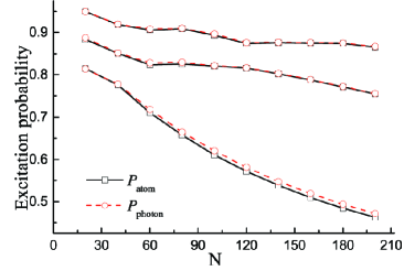
Figure 7: (Color online) The binary transmission probabilities verse the number of cavities with different $k$. From top to bottom, $k=8$, $k=4$, and $k=2$, with the system parameters are $\Delta=0$, $\lambda=10$, and $\xi=1$.

When the number of encoding qubits equals to that of decoding qubits, the maximum values of the excitation probabilities can be obtained. In Fig. 7, the maximum transfer probability is plotted as a function of $N$ for the class of encoding states. The curves show that the propagation fidelity increases rapidly as the number of encoding qubits $k$ increases. Clearly, the transmission probability decreases with respect to the cavity number $N$, and the decay becomes slower by encoding and decoding more qubits. The difference of excitation probabilities between atomic and photonic mode decreases as the number of encoding qubits increases. As is displayed in Fig. 7, the maximum probabilities of the binary transmission are higher than $0.86$ for $k=8$, even up to the $200$ cavities.

V CONCLUSION

To conclude, the dynamics of a cavity array is studied when each cavity contains a three-level atom. Adiabatically eliminating the intermediate state, the individual cavity can be described by the two-photon JC model with a metastable state and a ground state. By exploiting the metastable state, the transfer distance can be much longer than that of Jaynes-Cummings-Hubbard model at the expense of longer transmission times. When the adjacent cavities are coupled by two-photon hopping, the whole system Hamiltonian can be exactly diagonalized in the subspace of single-atom excitation. For the uniform and staggered intercavity hopping, we analyze the dynamics of the system in distinct regimes of parameters. With the staggered hopping, the excitation population trends to be localized in the first several cavities and slows down the transfer speed. This phenomenon becomes more distinct as the distortion of the hopping strength increases. Compared with the staggered hopping, the uniform hopping is more suitable for the quantum state transfer. In the strong hopping limit, only the photon is delocalized on the whole array of the coupled cavity with double speed. While in the strong coupling limit, the initial state in the first cavity plays an important role in the transmission fidelity for the binary transmission. Due to the strong coupling between atom and quantum field in individual cavity, the difference of maximum probabilities between the binary transmission is not very large. Finally, it is shown that a class of initial encodings and final decoding process used in spin system can also greatly improve the performance of binary transmission. The analysis of the dynamics in the high-Q optical cavities can also be exploited in analogous systems, such as circuit quantum electrodynamics and coupled photonic crystal cavities. The results of this work provide a step for studying the quantum state transfer in coupled cavities.

VI ACKNOWLEDGMENTS

This work is supported by the Specialized Research Fund for the Doctoral Program of Higher Education (Grant No. 20103201120002), Special Funds of the National Natural Science Foundation of China (Grant No. 11047168), the National Natural Science Foundation of China (Grant Nos. 11074184 and 11004144), the Natural Science Foundation of Jiangsu Province (Grant No. 10KJB140010), and the PAPD.

References

- (1) A. Zeilinger, A. Ekert, and D. Bouwmeester (editors), The Physics of Quantum Information: Quantum Cryptography, Quantum Teleportation, Quantum Computation (Springer, Berlin, 2000).
- (2) S. Lloyd, Science 261, 1569 (1993).
- (3) C. H. Bennett, G. Brassard, C. Crépeau, R. Jozsa, A. Peres, and W. K. Wootters, Phys. Rev. Lett. 70, 1895 (1993).
- (4) J. I. Cirac, P. Zoller, H. J. Kimble, and H. Mabuchi, Phys. Rev. Lett. 78, 3221 (1997).
- (5) A. D. Boozer, A. Boca, R. Miller, T. E. Northup, and H. J. Kimble, Phys. Rev. Lett. 98, 193601 (2007).
- (6) A. Muller, H. Zbinden, and N. Gisin, Europhys. Lett. 33, 335 (1996).
- (7) R. Ursin, F. Tiefenbacher, T. Schmitt-Manderbach, H. Weier, et al., Nat. Phys. 3, 481 (2007).
- (8) S. Bose, Phys. Rev. Lett. 91, 207901 (2003).
- (9) M. Christandl, N. Datta, A. Ekert, and A. J. Landahl, Phys. Rev. Lett. 92, 187902 (2004).
- (10) M. Christandl, N. Datta, T. C. Dorlas, A. Ekert, A. Kay, and A. J. Landahl, Phys. Rev. A 71, 032312 (2005).
- (11) S. G. Schirmer and P. J. Pemberton-Ross, Phys. Rev. A 80, 030301(R) (2009).
- (12) T. J. Osborne and N. Linden, Phys. Rev. A 69, 052315 (2004).
- (13) Z. M. Wang, C. Allen Bishop, M. S. Byrd, B. Shao, and J. Zou, Phys. Rev. A 80, 022330 (2009).
- (14) C. A. Bishop, Y. C. Ou, Z. M. Wang, and M. S. Byrd, Phys. Rev. A 81, 042313 (2010).
- (15) N. Y. Yao, L. Jiang, A. V. Gorshkov, Z. -X. Gong, A. Zhai, L. -M. Duan, and M. D. Lukin, Phys. Rev. Lett. 106, 040505 (2011).
- (16) H. J. Kimble, Nature (London) 453, 1023 (2008).
- (17) K. Hennessy, A. Badolato, M. Winger, D. Gerace, M. Atatue, S. Gulde, S. Falt, E. L. Hu, and A. Imamoglu, Nature (London) 445, 896 (2007).
- (18) R. J. Schoelkopf and S. M. Girvin, Nature (London) 451, 664 (2008).
- (19) A. Serafini, S. Mancini, and S. Bose, Phys. Rev. Lett. 96, 010503 (2006).
- (20) M. J. Hartmann, F. G. S. L. Brandão, and M. B. Plenio, Phys. Rev. Lett. 99, 160501 (2007).
- (21) J. Cho, D. G. Angelakis, and S. Bose, Phys. Rev. A 78, 062338 (2008).
- (22) Z. X. Chen, Z. W. Zhou, X. Zhou, X. F. Zhou, and G. C. Guo, Phys. Rev. A 81, 022303 (2010).
- (23) P. B. Li, Y. Gu, Q. H. Gong, and G. C. Guo, Phys. Rev. A 79, 042339 (2009).
- (24) M. J. Hartmann, F. G. S. L. Brandão, and M. B. Plenio, Nat. Phys. 2, 849 (2006).
- (25) A. D. Greentree, C. Tahan, J. H. Cole, and L. C. L. Hollenberg, Nat. Phys. 2, 856 (2006).
- (26) M. I. Makin, J. H. Cole, C. Tahan, L. C. L. Hollenberg, and A. D. Greentree, Phys. Rev. A 77, 053819 (2008).
- (27) C. D. Ogden, E. K. Irish, and M. S. Kim, Phys. Rev. A 78, 063805 (2008).
- (28) M. I. Makin, J. H. Cole, C. D. Hill, A. D. Greentree, and L. C. L. Hollenberg, Phys. Rev. A 80, 043842 (2009).
- (29) F. Ciccarello, Phys. Rev. A 83, 043802 (2011).
- (30) K. Zhang and Z. Y. Li, Phys. Rev. A 81, 033843 (2010).
- (31) W. L. Yang, Z. Q. Yin, Z. Y. Xu, M. Feng, and C. H. Oh, Phys. Rev. A 84, 043849 (2011).
- (32) J. T. Shen and S. Fan, Phys. Rev. Lett. 98, 153003 (2007).
- (33) D. Roy, Phys. Rev. Lett. 106, 053601 (2011).
- (34) J. Q. Liao and C. K. Law, Phys. Rev. A 82, 053836 (2010).
- (35) P. H. Mokler and R. W. Dunford, Physica Scripta. 69, C1 (2004).
- (36) M. T. C. Wong and C. K. Law, Phys. Rev. A 83, 055802 (2011).
- (37) M. Alexanian, Phys. Rev. A 81, 015805 (2010).
- (38) M. Alexanian, Phys. Rev. A 83, 023814 (2011).
- (39) V. Buzek and B. Hladky, J. Mod. Opt. 40, 1309 (1993).
- (40) M. Alexanian, S. K. Bose, and L. Chow, J. Mod. Opt. 45, 2519 (1998).
- (41) M. Brune, J. M. Raimond, P. Goy, L. Davidovich, and S. Haroche, Phys. Rev. Lett. 59, 1899 (1987).
- (42) A. Kay and D. G. Angelakis, Europhys. Lett. 84, 20001 (2008).
- (43) A. Kreuter, C. Becher, G. P. T. Lancaster, A. B. Mundt, C. Russo, H. Häffner, C. Roos, J. Eschner, F. Schmidt-Kaler, and R. Blatt, Phys. Rev. Lett. 92, 203002 (2004).
- (44) M. Šašura and V. Bužek, J. Mod. Optics. 49, 1593 (2002).
- (45) R. E. Peierls, Quantum Theory of Solids (Oxford University Press, London, 1955).
- (46) M. X. Huo, Y. Li, Z. Song, and C. P. Sun, Europhys. Lett. 84, 30004 (2008).
- (47) M. Horodecki, P. Horodecki, and R. Horodecki, Phys. Rev. A 60, 1888 (1999).