Scattering phase shifts for two particles

of different mass and non-zero total momentum

in lattice QCD

Luka Leskovec^(a) and Sasa Prelovsek^(b,a)

(a) Jozef Stefan Institute, Jamova 39, 1000 Ljubljana, Slovenia

(b) Faculty of Mathematics and Physics, University of Ljubljana, Jadranska 19, Ljubljana, Slovenia

e-mail: sasa.prelovsek@ijs.si

Abstract

We derive the relation between the scattering phase shift and the two-particle energy in the finite box, which is relevant for extracting the strong phase shifts in lattice QCD. We consider elastic scattering of two particles with different mass and with non-zero total momentum in the lattice frame. This is a generalization of the Lüscher formula, which considers zero total momentum, and the generalization of Rummukainen-Gottlieb’s formula, which considers degenerate particles with non-zero total momentum. We focus on the most relevant total momenta in practice, i.e. $\mathbf{P}=(2\pi/L)~{}e_{z}$ and $\mathbf{P}=(2\pi/L)~{}(e_{x}+e_{y})$ including their multiples and permutations. We find that the $P$-wave phase shift can be reliably extracted from the two-particle energy if the phase shifts for $l\geq 2$ can be neglected, and we present the corresponding relations. The reliable extraction of S-wave phase shift is much more challenging since $\delta_{l=0}$ is always accompanied by $\delta_{l=1}$ in the phase shift relations, and we propose strategies for estimating $\delta_{l=0}$. We also propose the quark-antiquark and meson-meson interpolators that transform according the considered irreducible representations.

1 Introduction

The phase shifts for strong elastic scattering of two hadrons encode the basic knowledge on the strong interaction between two hadrons, which is non-perturbative in its nature. The phase shift $\delta_{l}$ is related to the phase between the out-going and the in-going $l$-wave in the region outside the interaction range, and parametrizes our ignorance of the complicated form of this interaction. The phase shift indicates whether the interaction is attractive or repulsive, what is its strength as well as the range, and it provides the value of the scattering length. The knowledge of the phase-shift also serves to determine the masses and the width of the resonance that appears in the $l$-wave: $\delta_{l}=\pi/2$ at the resonance peak, while the sharpness of the rise allows the determination of the resonance width according to Breit-Wigner type functional form. In fact, the only feasible method for determining the resonance width on the lattice at present goes through the determination of the phase shift.

Two decades ago, Lüscher proposed how do determine phase shifts for elastic scattering in a lattice simulation [1]. He derived the phase shift relation, that relates the two-particle energy $E$ on a lattice of size $L$ and the infinite volume scattering phase shift $\delta_{l}(s)$, where $s=E^{2}-\mathbf{P}^{2}$ and $\mathbf{P}$ is the total three-momentum of two particles. If one determines two-particle energy $E$ from a lattice simulation with a given momentum $\mathbf{P}$, one can extract the phase shift $\delta(s)$ at particular $s=E^{2}-\mathbf{P}^{2}$ using this relation. Lüscher considered only the case $\mathbf{P}=0$. The explicit phase shift relations for higher $l$ at $\mathbf{P}=0$ ware written down in [2].

In order to determine $\delta(s)$ at more values of $s=E^{2}-\mathbf{P}^{2}$, one better considers also the case $\mathbf{P}\not=0$. The phase shift relations for this case were derived in [3, 6, 4, 5], but these consider the scattering of two particles with equal mass ($m_{1}=m_{2}$) .

In this paper we derive the phase shift relations for the general scattering of two particles with different mass ($m_{1}\not=m_{2}$) and with non-zero total momentum ($\mathbf{P}\not=0$). A first step in this direction was made by Davoudi and Savage [7] and by Fu [8], where the phase shift relation for the irreducible representation $A_{1}$ was written down: the relation in [7] takes into account only the $S$-wave interaction and neglects all higher partial waves, while the relation in [8] takes into account $S$ and $P$ wave. However, the $A_{1}$ representation is the least interesting in practice as it mixes $S$ and $P$-wave phase shifts in one relation if $\mathbf{P}\not=0$ and $m_{1}\not=m_{2}$, making it difficult to reliably extract any of the two. We derive the phase shift relations also for the other irreducible representations entering in $S$ or $P$-wave scattering with total momentum $\mathbf{P}=(2\pi/L)e_{z}$ and $\mathbf{P}=(2\pi/L)(e_{x}+e_{y})$: these representations do not mix $S$ and $P$-wave phase shifts. We also propose the form of lattice interpolators that transform according to these irreducible representations.

The analogous case of a moving bound state, which is composed of two particles with different mass, has been recently explored in [7, 9]. The corresponding finite volume corrections for the S-wave interaction of two particles has been derived in non-relativistic quantum mechanics [9] and in quantum field theory [7].

There have been a number of lattice simulations that extracted the phase shift using $\mathbf{P}=0$, or considering $\mathbf{P}\not=0$ but $m_{1}=m_{2}$. The $\pi\pi$ scattering with $I=2$ has been studied most frequently; see for example [10, 11] for $S$-wave at $\mathbf{P}\not=0$ and [12] for $D$-wave at $\mathbf{P}=0$. The $\rho$ resonance in $\pi\pi$ scattering with $I=1$ is the only resonance that has been clearly observed in the lattice studies of the phase shifts, which allowed the determination of its mass and width [13, 14, 15, 16, 17, 18]. The preliminary results for the challenging $\pi\pi$ scattering with $I=0$ were presented in [19, 20]. The $K\pi$ phase shift was extracted from the ground state with $\mathbf{P}=0$ [21], and the results on $I=3/2$ are more reliable than the $I=1/2$ ones. The analytic studies of the phase shift relations with $\mathbf{P}=0$ that may reveal the nature of the scalars mesons in these channels were presented in [22]. The $\rho\pi$ scattering and the related $a_{1}$ resonance ware simulated in [23], while the corresponding phase shift-relations for the scattering of unstable particles was analytically studied in [24]. The preliminary results for channels including charmed and charmonium states were presented in [25], while $D^{*}D_{1}$ scattering relevant for $Z^{+}(4430)$ was simulated in [26]. Recent review of the applications, including also baryons, multi-particle interactions and bound states was presented in [27].

There are however many interesting channels, where two scattering particles have different mass, and the simulations at non-zero total momentum would provide the valuable information on the corresponding phase shifts. To our knowledge, the phase shifts have not been extracted from lattice in such a case, and we provide analytical tools that would enable that in the near future.

In Section 2 we first consider two non-interacting particles in the finite volume, then we consider the interacting particles and write down the general phase shift relation. In Section 3 we simplify the general phase shift relations by considering the discrete symmetries. First we focus on the case of total momentum $\mathbf{P}=(2\pi/L)(e_{x}+e_{y})$, write down the phase shift relations for three irreducible representations that appear in $S$ or $P$-wave scattering, discuss the strategies for extracting the phase shifts $\delta_{l=0,1}$ and provide the quark-antiquark and meson-meson interpolators that transform according to these representations. Then we repeat the same steps for the total momentum $\mathbf{P}=(2\pi/L)e_{z}$. We end with conclusions. The Appendix provides the derivation of the expression for the generalized zeta function $Z_{lm}^{\mathbf{d}}(1;q^{2})$ for $m_{1}\not=m_{2}$, that is appropriate for numerical evaluation.

2 Two particles in a finite volume

We consider a square lattice box of volume $L^{3}$ with periodic boundary conditions in all three spatial directions, while time extent is infinite. We assume continuous space-time and we do not consider discretization errors due to the finite lattice spacing $a$ in actual simulations with a given action. There are two particles with total three-momentum $\mathbf{P}$ in such a box, and the total momentum has to satisfy the periodic boundary condition

$$\mathbf{P}=\mathbf{p}_{1}+\mathbf{p}_{2}\equiv\frac{2\pi}{L}\mathbf{d}\ ,\qquad\mathbf{d}\in Z^{3}~{}.$$ (1)

The main task is to derive the total energy $E$ of the these two particles, where $E$ refers to the energy measured by the observer that is at rest with respect to the lattice frame (LF), i.e. lattice square box. First we consider the non-interacting case, which is trivial. Then we turn to the interacting case, where the energy $E$ depends on the scattering phase shifts $\delta_{l}$ in the $l$-th partial wave. This relation will ultimately allow for the determination of $\delta_{l}$ from the energies determined by lattice simulations in a finite box.

The scattering in partial wave $l$ refers to the center-of-momentum frame (CMF), which moves with the velocity

$$\mathbf{v}=\frac{\mathbf{P}}{E}\quad,\qquad\gamma=\frac{1}{\sqrt{1-\mathbf{v}^{2}}}$$ (2)

with respect to the lattice frame. Therefore we need to consider the physical system in CMF, where the quantities will be denoted by $*$. The Lorentz transformation between two systems is performed by $\hat{\gamma}$, which acts on a general vector $\mathbf{u}$ as

$$\hat{\gamma}\mathbf{u}=\gamma\mathbf{u}_{\parallel}+\mathbf{u}_{\perp}~{},\quad\hat{\gamma}^{-1}\mathbf{u}=\gamma^{-1}\mathbf{u}_{\parallel}+\mathbf{u}_{\perp}~{},\qquad\mathbf{u}_{\parallel}=\tfrac{\mathbf{u}\cdot\mathbf{v}}{|\mathbf{v}^{2}|}~{}\mathbf{v}~{},\quad\mathbf{u}_{\perp}=\mathbf{u}-\mathbf{u}_{\parallel}$$ (3)

so it preserves the component perpendicular to $\mathbf{v}$ and modifies the component parallel to $\mathbf{v}$. The lattice square box is deformed to some general parallelepiped, and its shape depends on the direction of $\mathbf{P}$. The two-particle wave functions in CMF will “see” the lattice box in the shape of this parallelepiped and the technical difficulty is that the periodic boundary condition on the CMF wave functions has to be enforced with respect to this parallelepiped.

2.1 Non-interacting case

In the non-interacting case there are two major simplifications: the momenta of the individual particles also satisfy the periodic boundary condition and the energy is the sum of the individual energies

$$E=\sqrt{\mathbf{p}_{1}^{2}+m_{1}^{2}}~{}+\sqrt{\mathbf{p}_{2}^{2}+m_{2}^{2}}\ ,\qquad\mathbf{p}_{1}+\mathbf{p}_{2}=\mathbf{P}~{},\qquad\mathbf{p}_{1}=\frac{2\pi}{L}\mathbf{n}~{},\quad\mathbf{p}_{2}=\frac{2\pi}{L}\mathbf{n^{\prime}}~{},\qquad\mathbf{n},\mathbf{n^{\prime}}\in Z^{3}~{}.$$ (4)

This already provides the two-particle discrete energy spectrum in absence of interactions.

The energies of the interacting scattering states will be slightly shifted with respect to the non-interacting case (4). However the non-interacting case already gives us a rough estimate of the expected spectrum of scattering states and the corresponding values of $s=E^{2}-P^{2}$ in a simulation with given total momentum $\mathbf{P}$. The approximate knowledge on the allowed values of $s$ is very valuable, since such simulation would provide values of phase shifts $\delta(s)$ at those values of $s$. The allowed values of $\sqrt{s}$ for the non-interacting scattering states with $p_{1}\leq\sqrt{3}~{}\tfrac{2\pi}{L}$ and $p_{2}\leq\sqrt{3}~{}\tfrac{2\pi}{L}$ are presented in Fig. 1. In this example we take $m_{1}=200$ MeV, $m_{2}=500$ MeV (possible values of $m_{\pi}$ and $m_{K}$ in the present lattice simulations) and $L=3$ fm. The simulations with $\mathbf{P}=0$ will provide only the values of S-wave and P-wave phase shifts $\delta(s)$ at $\sqrt{s}\simeq\sqrt{m_{1}^{2}+n(\tfrac{2\pi}{L})^{2}}+\sqrt{m_{2}^{2}+n(\tfrac{2\pi}{L})^{2}}$ shown by circles; note that the lowest scattering state $P_{1}(0)P_{2}(0)$ is not present in P-wave. Simulations at $\mathbf{P}=\tfrac{2\pi}{L}e_{z}$ and $\mathbf{P}=\tfrac{2\pi}{L}(e_{x}+e_{y})$ will provide the values of S-wave and P-wave phase shifts at additional values of $\sqrt{s}$ given by the stars and triangles, respectively. Those values of $\sqrt{s}=\sqrt{E^{2}-\mathbf{P}^{2}}$ are obtained simply by using the energies $E$ (4) for certain values of $\mathbf{p}_{1}\in\tfrac{2\pi}{L}\mathbf{n}$ and $\mathbf{p}_{2}\in\tfrac{2\pi}{L}\mathbf{n^{\prime}}$. The allowed combinations of $\mathbf{p}_{1}$ and $\mathbf{p}_{2}$ will be understood only after we consider the symmetries of the two-particle system in CMF. For each irreducible representation they can be read off from the $P_{1}P_{2}$ interpolators given in (49) and (58).

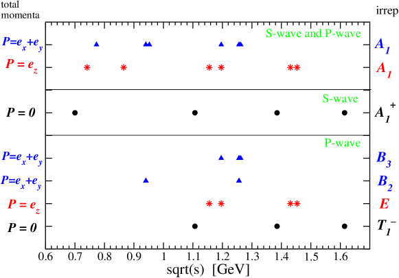
Figure 1: Values of the allowed $\sqrt{s}=\sqrt{E^{2}-P^{2}}$ for non-interacting scattering states of two particles with mass $m_{1}=200$ MeV, $m_{2}=500$ MeV and total momentum $\mathbf{P}$ in the lattice box of $L=3$ fm. Simulations at $P=0$ provide only the values of $\sqrt{s}$ given by the circles, while the simulations with $\mathbf{P}=\tfrac{2\pi}{L}e_{z}$ and $\mathbf{P}=\tfrac{2\pi}{L}(e_{x}+e_{y})$ provide also the values of $\sqrt{s}$ given by the stars and triangles, respectively. Each line corresponds to a definite irreducible representation in CMF, and corresponding $\sqrt{s}$ are obtained from $E$ (4) and choices of $\mathbf{p}_{1,2}$ in (49) and (58).

Since symmetries in CMF frame will be important, we also need the values of the allowed momenta $\mathbf{p}^{*}$ in the CMF frame for non-interacting case

$$\mathbf{p}^{*}=\mathbf{p}_{1}^{*}=-\mathbf{p}_{2}^{*}\qquad p^{*}=|\mathbf{p}^{*}|$$ (5)

to study the scattering. We extract $\mathbf{p}^{*}$ from $\mathbf{p}_{1}=\tfrac{2\pi}{L}\mathbf{n}$ using

$$\mathbf{p}_{1} =\hat{\gamma}(\mathbf{p}^{*}+\mathbf{v}E_{1}^{*})\ ,\qquad\mathbf{p}_{2}=\hat{\gamma}(-\mathbf{p}^{*}+\mathbf{v}E_{2}^{*})\qquad\mathrm{so}$$

$$\mathbf{p}^{*} =\hat{\gamma}^{-1}\mathbf{p}_{1}-\mathbf{v}E_{1}^{*}=\hat{\gamma}^{-1}[\mathbf{p}_{1}-\gamma\mathbf{v}E_{1}^{*}]=\hat{\gamma}^{-1}\biggl{(}\mathbf{p}_{1}-\gamma~{}\frac{2\pi\mathbf{d}}{LE}\frac{E^{*}}{2}~{}\bigl{[}1+\frac{m_{1}^{2}-m_{2}^{2}}{E^{*2}}\bigr{]}\biggr{)}$$

$$\mathbf{p}^{*} =\hat{\gamma}^{-1}~{}(\mathbf{p}_{1}-\tfrac{1}{2}~{}A~{}\mathbf{P})\ ,$$ (6)

where in the second step $E_{1}=(E^{*}/2)[1+(m_{1}^{2}-m_{2}^{2})/E^{*2}]$ is expressed in terms of energy in CMF

$$E^{*}=\sqrt{p^{*2}+m_{1}^{2}}+\sqrt{p^{*2}+m_{2}^{2}}=\gamma^{-1}~{}E~{}$$ (7)

and we have defined coefficient $A$

$$A\equiv 1+\frac{m_{1}^{2}-m_{2}^{2}}{E^{*2}}$$ (8)

which is different from $1$ only when $m_{1}\not=m_{2}$. We express the values of $\mathbf{p^{*}}$ in terms of the dimensionless CMF momentum $\mathbf{q}$

$$\mathbf{p}^{*}\equiv\frac{2\pi}{L}\mathbf{q}$$ (9)

and the allowed values of $\mathbf{q}$ in the non-interacting case are

$$\mathbf{q}=\mathbf{r}\qquad\mathbf{r}\in P_{d}\qquad\mathrm{(for\ non-interacting\ case)}$$ (10)

where the $\mathbf{r}\in P_{d}$ is set of vectors given by the mesh obtained combining (2.1,9,10) and $\mathbf{p}_{1}=\tfrac{2\pi}{L}\mathbf{n}$

$$P_{d}=\{~{}\mathbf{r}\quad|\quad\mathbf{r}=\hat{\gamma}^{-1}(\mathbf{n}-\tfrac{1}{2}~{}A~{}\mathbf{d})~{}\}\ ,\qquad\mathbf{n}\in Z^{3}~{}$$ (11)

which agrees with [7, 8]. The symmetries under which this set of points is invariant will play a major role later on. The equality $\mathbf{q}=\mathbf{r}$ (10) will be modified by the two-particle interactions in the finite volume.

2.2 Interacting case

Now we consider the elastic scattering of two interacting particles with spin 0 in a finite box using relativistic quantum mechanics, along the lines of Rummukainen-Gottlieb that consider $m_{1}=m_{2}$ [3], and Fu that presented the analogous derivation for $m_{1}\not=m_{2}$ [8].

For the case $m_{1}=m_{2}$, the quantum mechanics result of [3] was subsequently reproduced using the Bethe-Salpeter equation [6] and using the quantum field theory [4]. The phase shift relations from all approaches agree when one neglects the terms, that are exponentially suppressed with the box size $L$ in the quantum field theory. The phase shift relations derived here can therefore be applied if $L$ in the simulation is large enough that the terms of the order of $e^{-m_{\pi}L}$ can be neglected.

We need to find the two-particle energies $E$ in the finite box in the presence of the potential $V(\mathbf{x}^{*})$, which depends on their relative distance $\mathbf{x}^{*}=\mathbf{x}_{1}^{*}-\mathbf{x}_{2}^{*}$. The strong potential between two hadrons in not known ab-initio in QCD, so one can not analytically calculate the eigen-energies $E$ which satisfy $\hat{H}\psi(x_{1},x_{2})=E\psi(x_{1},x_{2})$, but rather determines eigen-energies $E$ in lattice QCD, which incorporates fundamental QCD interactions.

However, one can analytically consider the two-particle wave functions in the exterior region, where the potential drops to zero

$$V(\mathbf{x}^{*})=0\qquad\mathrm{for}\qquad|\mathbf{x}^{*}|=x^{*}>R$$ (12)

and we assume the interaction is of finite range $R<L/2$. In the exterior region, the two-particle wave function will satisfy $\hat{H}_{free}\psi_{free}(x_{1},x_{2})=E\psi_{free}(x_{1},x_{2})$ with the same eigen-energy $E$ as in the case of Hamiltonian $\hat{H}$ with interactions. The relation $\hat{H}_{free}\psi_{free}(x_{1},x_{2})=E\psi_{free}(x_{1},x_{2})$ in the exterior region of CMF has a form of the well-known Helmholtz equation

$$(\nabla^{2}+p^{*2})\phi_{CM}(\mathbf{x}^{*})=0\qquad x^{*}>R$$ (13)

$$E^{*}=\sqrt{p^{*2}+m_{1}^{2}}+\sqrt{p^{*2}+m_{2}^{2}}=\gamma^{-1}~{}E~{}$$ (14)

and the total energy $E^{*}$ is just a sum of both individual energies in this region.

The only effect of the interior region $x^{*}<R$ on the free solutions in the exterior region is that $\phi_{CM}(\mathbf{x}^{*})$ will depend on the phase shifts $\delta_{l}(p^{*})$, which are related to the phase between the out-going and in-going $l$-wave and parametrize our ignorance of the exact form of the potential $V(\mathbf{x}^{*})$. A free solution in the exterior region with momentum $p^{*}$, which is shifted by phase shift $\delta_{l}(p^{*})$, will satisfy the periodic boundary condition only for some specific values of $p^{*}$, which fulfill certain relation between $p^{*}$, $\delta_{l}(p^{*})$ and $L$. This relation is the analog of the Lüscher formula we are looking for: it will provide $\delta_{l}(p^{*})$ if one determines the momentum $p^{*}$ in the exterior region on a lattice of size $L$. This exterior momentum $p^{*}$ is extracted via relation (14) from the energy $E$ of two strongly interacting particles, where $E$ is directly measured with a lattice QCD simulation in a box of size $L$.

Before imposing the boundary conditions in the finite volume, let us review the familiar solutions of the Helmholtz equation for given $p^{*}$ in the infinite volume

$$\phi_{CM}(\mathbf{x}^{*})=\sum_{l,m}c_{lm}~{}Y_{lm}(\theta,\varphi)~{}[a_{l}(p^{*})j_{l}(p^{*}x^{*})+b_{l}(p^{*})n_{l}(p^{*}x^{*})]\ ,\qquad x^{*}>R~{},$$ (15)

which apply in the exterior region. The phase shift $\delta_{l}(p^{*})$ in the continuum is commonly defined through the ratio of the out-going $l$-wave $j_{l}-in_{l}$ and the in-going wave $j_{l}+in_{l}$ with momentum $p^{*}$

$$e^{2i\delta_{l}(p^{*})}\equiv\frac{a_{l}(p^{*})+ib_{l}(p^{*})}{a_{l}(p^{*})-ib_{l}(p^{*})}~{}.$$ (16)

We will use the same definition of the phase shift in the finite volume, but there the wave function will not be so simply expressed in terms of $j_{l}$ and $n_{l}$ due to the boundary conditions.

Now we turn to the solutions $\phi_{CM}(\mathbf{x}^{*})$ in the exterior region, that satisfy the Helmholtz equation and also the boundary condition at finite $L$. We consider the case of the periodic boundary condition in the lattice frame

$$\psi(\mathbf{x}_{1},\mathbf{x}_{2})=\psi(\mathbf{x}_{1}+\mathbf{n}_{1}L~{},~{}\mathbf{x}_{2}+\mathbf{n}_{2}L)$$ (17)

which is most commonly used in the actual simulations. These boundary conditions impose that $\phi_{CM}(\mathbf{x}^{*})$ need to satisfy the so-called $\mathbf{d}$-periodic boundary condition, which was derived by Fu [8] for $\mathbf{P}\not=0$ and $m_{1}\not=m_{2}$ using the Lorentz transformation between the two frames:

$$\phi_{CM}(\mathbf{x}^{*})=(-1)^{A\mathbf{n}\cdot\mathbf{d}}~{}\phi_{CM}(\mathbf{x}^{*}+\hat{\gamma}\mathbf{n}L)\qquad\mathbf{n}\in Z^{3}\ .$$ (18)

A simple example, that satisfies the Helmholtz equation and the $\mathbf{d}$-periodic boundary condition, is the Green function

$$G^{\mathbf{d}}(\mathbf{x}^{*},p^{*2})=\gamma^{-1}L^{-3}\sum_{k=\tfrac{2\pi}{L}\mathbf{r},~{}\mathbf{r}\in P_{d}}\frac{e^{i\mathbf{k}\cdot\mathbf{x}^{*}}}{\mathbf{k}^{2}-p^{*2}}$$ (19)

where $P_{d}$ is a mesh of points $P_{d}$ (11). Other solutions that satisfy the Helmholtz equation and the boundary conditions (18) are [1, 3, 8]

$$G_{lm}^{\mathbf{d}}(\mathbf{x}^{*},p^{*2})={\cal Y}_{lm}(\nabla)~{}G^{\mathbf{d}}(\mathbf{x}^{*},p^{*2})\ ,\qquad{\cal Y}_{lm}(\mathbf{x})\equiv x^{l}~{}Y_{lm}(\theta,\varphi)~{}.$$ (20)

The solutions $G_{lm}^{\mathbf{d}}$ form a complete basis, as shown by Lüscher for $\mathbf{d}=0$ [1], and the general solution $\phi_{CM}(\mathbf{x}^{*})$ can be expanded in terms of them

$$\phi_{CM}(\mathbf{x}^{*})=\sum_{l,m}v_{lm}~{}G_{lm}^{\mathbf{d}}(\mathbf{x}^{*},p^{*2})~{}\ ,\qquad x^{*}>R\ .$$ (21)

The technical difficulty arises from the fact that the solutions (21) satisfy boundary conditions (18) related to the parallelepiped in CMF, while the phase shifts $\delta_{l}$ are related to the coefficients in front of the out-going $j_{l}-in_{l}$ and in-going $j_{l}+in_{l}$ spherical waves as in the infinite volume (16). So one needs to express the $\mathbf{d}$-periodic solutions (20) in terms of the spherical Bessel functions $j_{l}$ and $n_{l}$. That can be fortunately done in analogous way as performed for $\mathbf{d}=0$ by Lüscher [1] and we omit the derivation here

$$G_{lm}^{\mathbf{d}}(\mathbf{x}^{*},p^{*2})=\frac{(-1)^{l}(p^{*})^{l+1}}{4\pi}\biggl{[}n_{l}(p^{*}x^{*})~{}Y_{lm}(\theta,\varphi)~{}+~{}\sum_{l^{\prime}=0}^{\infty}\sum_{m^{\prime}=-l^{\prime}}^{l^{\prime}}~{}{\cal M}_{lm,l^{\prime}m^{\prime}}^{\mathbf{d}}(q^{2})~{}j_{l^{\prime}}(p^{*}x^{*})~{}Y_{l^{\prime}m^{\prime}}(\theta,\varphi)\biggr{]}$$ (22)

where ${\cal M}_{lm,l^{\prime}m^{\prime}}^{d}(q^{2})$ are calculable matrices for given $l,~{}m,~{}l^{\prime},~{}m^{\prime},~{}\mathbf{d},~{}q\!=\!Lp^{*}/(2\pi)$ and $A$ (8) and the explicit expression will be given in the next section. The $\theta$ and $\varphi$ are polar angles of $\mathbf{x}^{*}$.

The general solution in the exterior region $\phi_{CM}(\mathbf{x}^{*})$ (21) is obtained by inserting (22), and one needs to relate this to the form (15) in order to extract the phase shifts defined by (16)

$$\phi_{CM}(\mathbf{x}^{*}) =\sum_{lm}v_{lm}\frac{(-1)^{l}(p^{*})^{l+1}}{4\pi}\biggl{[}n_{l}(p^{*}x^{*})~{}Y_{lm}(\theta,\varphi)~{}+~{}\sum_{l^{\prime},m^{\prime}}~{}{\cal M}_{lm,l^{\prime}m^{\prime}}^{\mathbf{d}}(q^{2})~{}j_{l^{\prime}}(p^{*}x^{*})~{}Y_{l^{\prime}m^{\prime}}(\theta,\varphi)\biggr{]}$$

$$=\sum_{l,m}c_{lm}~{}Y_{lm}(\theta,\varphi)~{}[a_{l}(p^{*})j_{l}(p^{*}x^{*})+b_{l}(p^{*})n_{l}(p^{*}x^{*})]\ ,\qquad x^{*}>R\ .$$ (23)

By equating the terms in from of $Y_{lm}n_{l}$ and $Y_{lm}j_{l}$ we get two relations

$$v_{lm}\frac{(-1)^{l}(p^{*})^{l+1}}{4\pi}=c_{lm}~{}b_{l}(p^{*})\ ,\qquad\sum_{l^{\prime},m^{\prime}}v_{l^{\prime}m^{\prime}}\frac{(-1)^{l^{\prime}}(p^{*})^{l^{\prime}+1}}{4\pi}{\cal M}_{l^{\prime}m^{\prime},lm}(q^{2})=c_{lm}~{}a_{l}(p^{*})~{}$$ (24)

and $v_{lm}$ can be expressed from the first relation and inserted into the second

$$\sum_{l^{\prime},m^{\prime}}c_{l^{\prime}m^{\prime}}\bigl{[}b_{l^{\prime}}(p^{*})~{}{\cal M}_{l^{\prime}m^{\prime},lm}(q^{2})-a_{l^{\prime}}(p^{*})\delta_{ll^{\prime}}\delta_{mm^{\prime}}\bigr{]}=0\ .$$ (25)

This linear system has nontrivial solution for $c_{l^{\prime}m^{\prime}}$ only if

$$det(BM-A)=0\qquad A_{lm,l^{\prime}m^{\prime}}\equiv a_{l}(p^{*})\delta_{ll^{\prime}}\delta_{mm^{\prime}}\ ,\quad B_{lm,l^{\prime}m^{\prime}}\equiv b_{l}(p^{*})\delta_{ll^{\prime}}\delta_{mm^{\prime}}\$$ (26)

where $A$ and $B$ are defined as diagonal matrices related to coefficients $a_{l}$ and $b_{l}$ [1] and they finally provide the information on the phase $\delta_{l}$ defined by (16)

$$e^{2i\delta}=\frac{A+iB}{A-iB}~{}.$$ (27)

By dividing (26) by $det(A-iB)$, which is non-zero [1], one obtains the final relation between the diagonal matrix $e^{2i\delta}$ and (in general) non-diagonal matrix $M$

$$det[e^{2i\delta}(M-i)-(M+i)]=0\ ,\qquad\qquad\quad l,l^{\prime}\leq l_{max}$$ (28)

$$\quad M_{lm,l^{\prime}m^{\prime}}\equiv {\cal M}^{\mathbf{d}}_{lm,l^{\prime}m^{\prime}}(q^{2})\ ,\quad[e^{2i\delta}]_{lm,l^{\prime}m^{\prime}}\equiv e^{2i\delta_{l}(p^{*})}\delta_{ll^{\prime}}\delta_{mm^{\prime}}\ .$$

This condition is the heart of the phase shift relation and relates the energy $E$ (or $q$) measured on the lattice to the unknown phases $\delta_{l}(p^{*})$ via the calculable matrix elements ${\cal M}^{\mathbf{d}}_{lm,l^{\prime}m^{\prime}}(q^{2})$, that will be given in the next subsection. The energy level $E$ will provide the information on the phase shift $\delta_{l}(p^{*})$ at CMF momentum $p^{*}$, that is related to $E$ via (14).

If $\delta_{l}=0$ for $l>l_{max}$, the relation (28) needs to be satisfied for the truncated square matrices with $l,l^{\prime}\leq l_{max}$, as shown in [4].

The determinant of the block-diagonal matrix is a product of determinants for separate blocks. So the determinant condition will get simplified when $M$ will be written in such basis that leads to a block-diagonal form of $M$ and therefore block-diagonal form of $e^{2i\delta}(M\!-\!i)-(M\!+\!i)$.

2.3 Definitions of ${\cal M}^{\mathbf{d}}_{lm,l^{\prime}m^{\prime}}$ and $Z_{lm}^{d}$ for $m_{1}\not=m_{2}$

Finally we write down the explicit expression for ${\cal M}^{\mathbf{d}}_{lm,l^{\prime}m^{\prime}}(q^{2})$, that were introduced while expanding $G^{\mathbf{d}}_{lm}$ in terms of $j_{l}$ and $n_{l}$ (22) [1, 3, 8]

$${\cal M}^{\mathbf{d}}_{lm,l^{\prime}m^{\prime}}(q^{2}) \equiv\frac{(-1)^{l}}{\gamma\pi^{3/2}}\sum_{j=|l-l^{\prime}|}^{l+l^{\prime}}\sum_{s=-j}^{j}\frac{i^{j}}{q^{j+1}}Z_{js}^{\mathbf{d}}(1;q^{2})~{}C_{lm,js,l^{\prime}m^{\prime}}\ ,$$ (29)

$$C_{lm,js,l^{\prime}m^{\prime}} \equiv(-1)^{m^{\prime}}i^{l-j+l^{\prime}}\sqrt{(2l+1)(2j+1)(2l^{\prime}+1)}\biggl{(}{l\atop m}{j\atop s}{l^{\prime}\atop-m^{\prime}}\biggr{)}\biggl{(}{l\atop 0}{j\atop 0}{l^{\prime}\atop 0}\biggr{)}\ ,$$

where $C_{lm,js,l^{\prime}m^{\prime}}$ is expressed in terms of the $3j$-Wigner symbols. The modified zeta function is defined as in [7, 8]

$$Z^{\mathbf{d}}_{lm}(s;q^{2})\equiv\sum_{\mathbf{r}\in P_{d}}\frac{{\cal Y}_{lm}(\mathbf{r})}{(\mathbf{r}^{2}-q^{2})^{s}}\ ,$$ (30)

where $P_{d}$ is the mesh of points defined in (11), and ${\cal Y}_{lm}$ is defined in (20). In the special case $\mathbf{d}=0$, the definition of the zeta function (30) agrees with the original definition by Lüscher [1]. The zeta function depends on $l,~{}m$, $q^{2}=(Lp^{*}/2\pi)^{2}$, $\mathbf{d}$ and $A$ (8). The $Z_{00}$ is finite only for $s>3/2$, but the divergence is not physical as it cancels in the difference between the finite and infinite volume result, as explained in the Appendix A, where $Z_{00}^{\mathbf{d}}$ is obtained by analytical continuation from $s>3/2$ to $s=1$. The $Z_{lm}^{\mathbf{d}}(1;q^{2})$ is finite for $l\not=0$, but the sum (30) converges to slowly for practical evaluation. In Appendix A we derive an expression that is suitable for the numerical evaluation and reproduces the known result in the special case $m_{1}=m_{2}$ [3, 5, 15].

2.4 General form of $M$ for $l_{max}=1$

In this paper we are especially interested in extracting the $S$ and $P$-wave phase shifts $\delta_{l=0,1}(p^{*})$ for the scattering of two particles with different mass. This problem is significantly simplified if the scattering phases for the partial waves with $l>l_{max}=1$ are small and can be neglected, i.e. we will assume that $\delta_{l>1}=0$. This is generally true for small $p^{*}$, where higher partial waves are generally suppressed by $\delta(p^{*})\propto(p^{*})^{2l+1}$ and is often true also for a range of $p^{*}$ if there is no $D$-wave resonance in the vicinity. The phases for the higher partial waves were explicitly found to be small for $p^{*}\geq 1$ GeV in the simulation [12] of the non-resonant channel $\pi\pi$ with $I=2$.

Assuming $\delta_{l>1}=0$, the matrix $M$ is $4\times 4$ matrix in the basis $lm=00,10,11,1-1$ and the expression ${\cal M}_{lm,l^{\prime}m^{\prime}}^{\mathbf{d}}$ (29) leads to the following form for general $\mathbf{d}$

$$M={\cal M}_{lm,l^{\prime}m^{\prime}}^{\mathbf{d}}=\bordermatrix{~{}&00&10&11&1-1\cr 00&w_{00}&i\sqrt{3}w_{10}&i\sqrt{3}w_{11}&i\sqrt{3}w_{1-1}\cr 10&-i\sqrt{3}w_{10}&w_{00}+2w_{20}&\sqrt{3}w_{21}&\sqrt{3}w_{2-1}\cr 11&i\sqrt{3}w_{1-1}&-\sqrt{3}w_{2-1}&w_{00}-w_{20}&-\sqrt{6}w_{2-2}\cr 1-1&i\sqrt{3}w_{11}&-\sqrt{3}w_{21}&-\sqrt{6}w_{22}&w_{00}-w_{20}\cr}\ ,$$ (31)

where we defined $w_{lm}$ to simplify the notation

$$w_{lm}\equiv\frac{1}{\pi^{3/2}\sqrt{2l+1}~{}\gamma~{}q^{l+1}}~{}Z_{lm}^{\mathbf{d}}(1;q^{2})\ .$$ (32)

3 Consequences of the discrete symmetries of mesh $P_{d}$

Some of the matrix elements ${\cal M}_{lm,l^{\prime}m^{\prime}}^{\mathbf{d}}$ (31) are zero for particular choices of $\mathbf{d}$, which becomes apparent after explicit numerical evaluation of the $w_{lm}\propto Z^{\mathbf{d}}_{lm}(1;q^{2})$ given in Appendix A. This is a consequence of the discrete symmetries of the mesh $P_{d}$ (11) in CMF. It is helpful to first study these symmetries and determine the texture of the matrix ${\cal M}$ (31) for particular $\mathbf{d}$ before inserting $M$ to the master determinant condition (28).

So we explore in this section the group $G$ of the symmetry elements $\hat{R}$ that leaves the mesh $P_{d}$ (11) invariant. Later on we study the consequences of these symmetries for two most useful types of non-zero momentum $\mathbf{d}\propto e_{z}$ and $\mathbf{d}\propto e_{x}+e_{y}$, or permutations. There are several reasons why symmetry consideration will be helpful:

• It will indicate which $Z_{lm}^{\mathbf{d}}$ are zero, purely real or purely imaginary, as indicated above.

• The Helmholtz solution $G^{\mathbf{d}}$ (19) is invariant under the transformations $\hat{R}\in G$ due to the sum over $\mathbf{r}\in P_{d}$. The other solutions $G_{lm}^{\mathbf{d}}$ are generated by applying ${\cal Y}_{lm}(\nabla)$, so they transform like $Y_{lm}$ [1, 5]

  $$G^{\mathbf{d}}_{lm}(\hat{R}\mathbf{x}^{*},p^{*2})=\sum_{m^{\prime}=-l}^{l}D_{mm^{\prime}}^{(l)}(\hat{R})~{}G^{\mathbf{d}}_{lm^{\prime}}(\mathbf{x}^{*},p^{*2})\ ,$$ (33)

  where $D_{mm^{\prime}}^{(l)}(\hat{R})$ is defined as a representation in the bases $Y_{lm}$

  $$Y_{lm}(\hat{R}\mathbf{x})=\sum_{m^{\prime}=-l}^{l}D_{mm^{\prime}}^{(l)}(\hat{R})Y_{lm^{\prime}}(\mathbf{x})$$ (34)

  and is in general reducible. So the solutions $G^{\mathbf{d}}_{lm}$ form a representation of group $G$, which is in general reducible. The energy eigenstates in (21) are certain linear combinations of $G^{\mathbf{d}}_{lm}$ that transform according to the irreducible representation of the $G$; the representation $D_{mm^{\prime}}^{(l)}(\hat{R})$ of transformation $\hat{R}$ (33) has the irreducible block-diagonal form in this basis.

• The same linear combinations of $Y_{lm}$ will also lead to the block-diagonal form of $M$, as shown by Lüscher (see section n5.3 of [1]). We will therefore write down $M$ and search for the basis that leads to the block-diagonal form. It will turn out that the resulting basis indeed corresponds to the irreducible representations of $D$ (33,34).

• The determinant condition (28) is greatly simplified in the bases where $M$ is block-diagonal since the determinant of the block-diagonal matrix is a product of determinants for separate blocks. In this case the determinant condition is simplified to analogous conditions for separate blocks (i.e. irreducible representations).

• The lattice interpolators, that are written down in the lattice frame, have to transform according to the irreducible representation of the group $G$ after transformed to the CMF frame. We will provide useful examples of quark-antiquark and meson-meson interpolators, that satisfy this property and be used in the actual simulations to extract the phase shifts.

All these reasons prompt us to consider the symmetries of the mesh $P_{d}$ (11) for separate cases of $\mathbf{d}$.

       

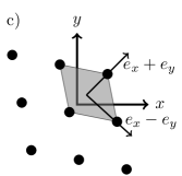
Figure 2: The mesh $P_{d}$ (11) for $\mathbf{d}=e_{x}+e_{y}$ and $m_{1}\not=m_{2}$ ($A\not=1$) is plotted in (c), while (a) and (b) show the steps how to get it.

3.1 $\mathbf{P}=(2\pi/L)(e_{x}+e_{y})$ and consequences of $C_{2v}$ symmetries

We first explain the case of the momentum $\mathbf{d}=e_{x}+e_{y}$ in detail, since it is general enough to illustrate the procedure and since the corresponding group has only few elements. All the results can be easily generalized to the case $\mathbf{d}=N(e_{x}+e_{y})$ or any permutation in the direction.

We first need to determine the symmetry transformations $\hat{R}$ that leave $P_{d}$ invariant. The mesh $P_{d}$ (11) can be visualized in Fig. 2c and is obtained in two steps:

1. First the cubic mesh $\mathbf{r}=\mathbf{n}\in Z^{3}$ in Fig. 2a is shifted by $-\tfrac{1}{2}A\mathbf{d}\propto e_{x}+e_{y}$ and since $A\not=1$ for $m_{1}\not=m_{2}$ (8), the origin is not in the center of the unit cell in $xy$ plane (Fig. 2b). The inversion $I$ with respect to the origin is lost as a symmetry at this stage, so the corresponding group $G$ will not contain $I$; this is a major difference with respect to degenerate case $m_{1}=m_{2}$, when the origin is at the center of the unit cell in $xy$ plane and $I$ is the symmetry. We will see that this has important consequences, for example that sectors with even and odd $l$ will not decouple, which will present challenges in certain cases.

2. In the second step $\hat{\gamma}^{-1}$ contracts the distances in the direction $\mathbf{v}\propto e_{x}+e_{y}$ and keeps the distances perpendicular to that, so the mesh is not modified in $z$ direction.

The resulting unit cell in Fig. 2c has the form of rhombic prism and the mesh $P_{d}$ is invariant only under four transformations $\hat{R}$ listed in Table 1. There $Id$ denotes the identity, $C_{n}(\mathbf{V})$ denotes a rotation by $2\pi/n$ around $\mathbf{V}$, while $\sigma(\mathbf{V})$ denotes the reflection with respect to the plane perpendicular to $\mathbf{V}$. These four transformations form group $C_{2v}$, which has only one-dimensional irreducible representations. For the one-dimensional irreducible representation ”irrep” the transformation $\hat{R}$ on a vector $\mathbf{u}$ is given by the character $\chi^{irrep}(\hat{R})$

$$\hat{R}~{}\mathbf{u}=\chi^{irrep}(\hat{R})~{}\mathbf{u}\ ,\quad\chi^{irrep}(\hat{R})=\pm 1\ ,\qquad\mathrm{for\ 1D\ irrep}\ .$$ (35)

The characters of the irreducible ($A_{1,2},B_{2,3}$) and reducible ($lm$) representations are given in Table 1 along with an example of polynomials and vectors $\mathbf{u}$ that transform according to these representations.

respresent.	dim	$Id$	$C_{2}(e_{x}+e_{y})$	$\sigma(e_{x}-e_{y})$	$\sigma(e_{z})$	polynom.	vector $\mathbf{u}$
irred. $A_{1}$	1	1	1	1	1	1 , $x+y$	$\mathbf{0}$, $e_{x}+e_{y}$
irred. $A_{2}$	1	1	1	-1	-1	$(l>1)$	$(l>1)$
irred. $B_{3}$	1	1	-1	1	-1	$z$	$e_{z}$
irred. $B_{2}$	1	1	-1	-1	1	$x-y$	$e_{x}-e_{y}$
$\Gamma^{l=0}$	1	1	1	1	1	$Y_{00}$
$\Gamma^{l=1}$	3	3	-1	1	1	$Y_{10},Y_{11},Y_{1-1}$

Table 1: Characters $\chi(\hat{R})=\sum_{i=1}^{dim}D(\hat{R})_{ii}$ of representations $D$ for transformations $\hat{R}\in C_{2v}$ (with principal axis $e_{x}+e_{y}$), that leave the mesh $P_{d}$ in Fig. 2 for $\mathbf{d}=e_{x}+e_{y}$ invariant. Representations $A_{1,2}$ and $B_{2,3}$ are irreducible while the representation $\Gamma^{l=1}$ is reducible. Example of polynomials and vectors $\mathbf{u}$ that transform according to these representations are given on the right.

The functions $Y_{lm}$ (34) and also the solutions $G_{lm}^{\mathbf{d}}$ (33) form a representation $\Gamma^{(l)}$ for transformations $\hat{R}\in C_{2v}$, but the $2l+1$ dimensional representation $\Gamma^{(l)}$ with $m=-l,..,l$ is in general reducible. We will need the number of times ($N^{irrep}$) that irreducible representation “irrep” enters in $\Gamma^{(l)}$ [29]

$$N^{irrep}=\frac{1}{g}\sum_{\hat{R}}\chi^{irrep}(\hat{R})^{*}~{}\chi^{(l)}(\hat{R})\ ,$$ (36)

where $g$ is the number of elements $\hat{R}$ of the group $G$, while the characters of irreducible representations $\chi^{irrep}(\hat{R})$ and reducible representations $\chi^{(l)}(\hat{R})$ are given in Table 1. The resulting decomposition is

$$\Gamma^{(0)} =A_{1}$$ (37)

$$\Gamma^{(1)} =A_{1}\oplus B_{3}\oplus B_{2}$$

$$\Gamma^{(2)} =2A_{1}\oplus A_{2}\oplus B_{3}\oplus B_{2}$$

This indicates that the solutions (and also interpolators) that transform according to the listed irreps will contain the following partial waves

$$B_{3}:\ l=1,~{}2,..\qquad B_{2}:\ l=1,~{}2,..\qquad A_{1}:\ l=0,~{}1,~{}2,..\qquad A_{2}:\ l=2,..$$ (38)

so $B_{3}$ or $B_{2}$ in CMF will couple to $l=1$, but not to $l=0$. These two representations therefore provide a rather clean possibility to extract $l=1$ phase shift if partial waves with $l>1$ can be neglected. The interpolators that transform according to irrep $A_{1}$ in CMF will couple to both $l=0$ and $l=1$, and there is unfortunately no irreducible representation which would couple only to $l=0$. This will present a serious challenge for a reliable extraction of $l=0$ phase shift in simulations with non-zero total momentum, as will be discussed in more detail later on.

The mixing between the even and odd $l$ occurs since inversion is not an element of the group $C_{2v}$ (see Table 1). We emphasize that this mixing is not present for the scattering of particles with $m_{1}=m_{2}$ and total momentum $\mathbf{d}=e_{x}+e_{y}$ since inversion is element of $D_{2h}$: $A^{+}$ contains only the waves $l=0,2$ and $l\geq 4$, while $B_{1,2,3}^{-}$ contains only $l=1$ and $l\geq 3$ [5]. This mixing is also not present for the scattering of particles with $m_{1}\not=m_{2}$ and total momentum $\mathbf{P}=0$, where $A_{1}^{+}$ contains only $l=0,4,..$ and $T_{1}^{-}$ contains only $l=1,3,..$ [1].

3.1.1 Values of $Z_{lm}^{\mathbf{d}}$ as consequences of the symmetries for $\mathbf{d}=e_{x}+e_{y}$

The transformations $\hat{R}\in C_{2v}$ leave the mesh $P_{d}$ invariant, so the sum over $\mathbf{r}\in P_{d}$ in $Z_{lm}$ (30) can be replaced by the sum over $\mathbf{r}^{\prime}=\hat{R}\mathbf{r}$

$$Z_{lm}^{\mathbf{d}}(q^{2}) =\sum_{\mathbf{r}}\frac{{\cal Y}_{lm}(\mathbf{r})}{(\mathbf{r}^{2}-q^{2})^{s}}=\sum_{\mathbf{r}^{\prime}=\hat{R}\mathbf{r}}\frac{|\mathbf{r}^{\prime}|^{l}~{}{Y}_{lm}(\mathbf{r}^{\prime})}{(\mathbf{r}^{\prime 2}-q^{2})^{s}}=\sum_{\mathbf{r}}\frac{\mathbf{r}^{l}~{}Y_{lm}(R\mathbf{r})}{(\mathbf{r}^{2}-q^{2})^{s}}\qquad\mathrm{since}\ |\mathbf{r}^{\prime}|=|\hat{R}\mathbf{r}|=|\mathbf{r}|$$ (39)

which will have important consequences for some $\hat{R}$. Now we can list the properties of $Z^{\mathbf{d}}_{lm}$ for $\mathbf{d}=e_{x}+e_{y}$:

• $Z^{\mathbf{d}}_{l~{}-m}=(-1)^{m}(Z^{\mathbf{d}}_{lm})^{*}$ which is the consequence of the analogous relation for $Y_{lm}$.

• $Z^{\mathbf{d}}_{lm}=i^{m}(Z^{\mathbf{d}}_{lm})^{*}$ since $\hat{R}=\sigma(e_{x}-e_{y})\in C_{2v}$:

  The reflection $\hat{R}=\sigma(e_{x}-e_{y})$ with respect to the plane perpendicular to $e_{x}-e_{y}$ transforms $x\to y,~{}y\to x,~{}z\to z$ or equivalently $\theta\to\theta,\ e^{i\varphi}\propto x+iy\to y+ix=i(x-iy)\propto ie^{-i\varphi}$. This transforms $Y_{lm}\equiv f(\theta)~{}(e^{i\varphi})^{m}~{}\to~{}f(\theta)(ie^{-i\varphi})^{m}=f(\theta)i^{m}e^{-im\varphi}=i^{m}(Y_{lm})^{*}$ and then (39) leads to $Z_{lm}^{\mathbf{d}}=i^{m}(Z^{\mathbf{d}}_{lm})^{*}$.

  Rewriting $Z^{\mathbf{d}}_{lm}=Re(Z^{\mathbf{d}}_{lm})+i~{}Im(Z^{\mathbf{d}}_{lm})$ this leads to $Im(Z^{\mathbf{d}}_{lm})=0$ for $m=0,4,..$, $Re(Z^{\mathbf{d}}_{lm})=Im(Z^{\mathbf{d}}_{lm})$ for $m=1,5,..$, $Re(Z^{\mathbf{d}}_{lm})=0$ for $m=2,6,..$ and $Re(Z^{\mathbf{d}}_{lm})=-Im(Z^{\mathbf{d}}_{lm})$ for $l=3,7,..$, independent of the value of $l$.

  This property of $Z^{\mathbf{d}}_{lm}$ holds for any case where the mesh $P_{d}$ is symmetric under $\hat{R}=\sigma(e_{x}-e_{y})$, which is true for all $\mathbf{d}=0,~{}e_{x}+e_{y},~{}e_{z}$ in case of degenerate or non-degenerate masses.

• $Z_{lm}^{\mathbf{d}}=0$ for $l-m=odd$ since $\sigma(e_{z})\in C_{2v}$:

  The reflection $\hat{R}=\sigma(e_{z})$ with respect $xy$ plane transforms $\theta\to\pi-\theta$ and $\varphi\to\varphi$, while $Y_{lm}(\pi-\theta,\varphi)=(-1)^{l-m}Y_{lm}(\theta,\varphi)$ so (39) leads to $Z_{lm}^{\mathbf{d}}=(-1)^{l-m}Z_{lm}^{\mathbf{d}}$.

• Note that if inversion $I$ would be in $G$ then $Z^{\mathbf{d}}_{lm}=(-1)^{l}Z^{\mathbf{d}}_{lm}$ or $Z^{\mathbf{d}}_{lm}=0$ for odd $l$. This would decouple parts of $M$ for even and odd $l$. In the present case $m_{1}\not=m_{2}$ and $\mathbf{d}\not=0$, so $I$ is not element of $G$ and $Z_{lm}^{\mathbf{d}}$ is not zero in general for odd $l$.

We verified all the above relations to be true also with the explicit numerical evaluation of $Z^{\mathbf{d}}_{lm}$ using the expression in Appendix A. For example $Z^{\mathbf{d}}_{11}(m_{1}\not=m_{2})\not=0$ and has equal real and imaginary part, while $Z^{\mathbf{d}}_{11}(m_{1}=m_{2})=0$ as required by the symmetries of $D_{2h}$ for the mass-degenerate case [5].

3.1.2 The matrix ${\cal M}_{lm,l^{\prime}m^{\prime}}^{\mathbf{d}}$ for $\mathbf{d}=e_{x}+e_{y}$

The above relations for $Z_{lm}^{\mathbf{d}}$ or equivalently $w_{lm}$ (32) simplify the general matrix ${\cal M}$ (31) to

$$M={\cal M}_{lm,l^{\prime}m^{\prime}}^{\mathbf{d}}=\bordermatrix{~{}&00&10&11&1-1\cr 00&w_{00}&0&i\sqrt{3}w_{11}&-\sqrt{3}w_{11}\cr 10&0&w_{00}+2w_{20}&0&0\cr 11&-\sqrt{3}w_{11}&0&w_{00}-w_{20}&\sqrt{6}w_{22}\cr 1-1&i\sqrt{3}w_{11}&0&-\sqrt{6}w_{22}&w_{00}-w_{20}\cr}$$ (40)

since $iw_{1-1}=-iw_{11}^{*}=-w_{11}$ due to $Re(w_{11})=Im(w_{11})$, and $w_{2-2}=w_{22}^{*}=-w_{22}$ due to $Re(w_{22})=0$, while $w_{00}$ and $w_{20}$ are real.

3.1.3 Phase shift relations for $\mathbf{d}=e_{x}+e_{y}$

The phase shift relations are obtained from the determinant condition (28), which gets simplified when $M$ (40) is written in the basis that renders it block-diagonal.

Extracting $P$-wave phase shift from irreps $B_{3}$ or $B_{2}$

The part $Y_{10}\propto z$ already presents a separate block, which transforms according to $B_{3}$: $z$ gets multiplied by $-1$ for reflection with respect to $xy$ plane and rotation around $e_{x}+e_{y}$ and stays invariant for other two transformations (see Table 1). The determinant condition for this $1\times 1$ block requires $det[e^{2i\delta_{1}}(M^{B_{3}}\!-\!i)-(M^{B_{3}}\!+\!i)]=0$ or equivalently $\tan(\delta_{1})=1/M^{B_{3}}$ with $M^{B_{3}}=w_{00}+2w_{20}$, so

$$\mathbf{d}=e_{x}+e_{y}~{},\ B_{3}\ \mathrm{of}\ C_{2v}\ :\quad\tan\delta_{1}(p^{*})=\frac{\pi^{3/2}~{}\gamma~{}q}{Z_{00}^{\mathbf{d}}(1;q^{2})+\tfrac{2}{\sqrt{5}}~{}q^{-2}~{}Z_{20}^{\mathbf{d}}(1;q^{2})}\ .$$ (41)

This is the final relation that allows the determination of $P$-wave phase shift $\delta_{1}(p^{*})$ from the energy $E$ of two particles with total momentum $\mathbf{P}=\tfrac{2\pi}{L}(e_{x}+e_{y})$ when one uses the interpolators that transform according to $B_{3}$.

The eigenvectors of the remaining $3\times 3$ matrix $M$ (40) reveal that one simple eigenvector is $\mathbf{u}^{B_{2}}=\tfrac{1}{\sqrt{2}}(-iY_{11}+Y_{1-1})\propto x-y$ which transforms according to $B_{2}$ (see Table 1). The corresponding eigenvalue is $M^{B_{2}}=w_{00}-w_{20}-\sqrt{6}Im(w_{22})$ and the determinant condition (28) for this $1\times 1$ block gives $\tan(\delta_{1})=1/M^{B_{3}}$ , or

$$\mathbf{d}=e_{x}+e_{y}~{},\ B_{2}\ \mathrm{of}\ C_{2v}~{}:\quad\tan\delta_{1}(p^{*})=\frac{\pi^{3/2}~{}\gamma~{}q}{Z_{00}^{\mathbf{d}}(1;q^{2})-\tfrac{1}{\sqrt{5}}~{}q^{-2}~{}Z_{20}^{\mathbf{d}}(1;q^{2})-\tfrac{\sqrt{6}}{\sqrt{5}}~{}q^{-2}~{}Im[Z_{22}^{\mathbf{d}}(1;q^{2})]}.$$ (42)

This is another relation that allows determination of $\delta_{1}(p^{*})$ when using interpolators in irrep $B_{2}$.

The phase shift relations for irreps $B_{3}$ (41) and $B_{2}$ (42) agree with the expressions in [5, 15] for the case $m_{1}=m_{2}$. The remaining representations, discussed bellow, have different role in the $m_{1}=m_{2}$ and $m_{1}\not=m_{2}$ cases.

Problems and strategies for extracting $S$-wave phase shift from irrep $A_{1}$

The remaining $2\times 2$ matrix ${M}$ can not be reduced further and spans the space in the basis of vectors $\mathbf{u}^{A_{1}}_{1}=\tfrac{1}{\sqrt{2}}(Y_{11}-iY_{1-1})\propto x+y$ and $\mathbf{u}^{A_{1}}_{2}=Y_{00}\propto 1$, which are perpendicular to the vectors $\mathbf{u}^{B_{3}}=Y_{10}$ and $\mathbf{v}^{B_{2}}$ above. The vectors $x+y$ and $1$ both remain invariant under all four $\hat{R}\in C_{2v}$ and belong to $A_{1}$ irreducible representation (see Table 1). The remaining $2\times 2$ block in the basis $\mathbf{u}^{A_{1}}_{1,2}$ is contained in

$$M_{ab}^{B}=\bordermatrix{~{}&Y_{00}&\tfrac{Y_{11}-iY_{1-1}}{\sqrt{2}}&Y_{10}&\tfrac{-iY_{11}+Y_{1-1}}{\sqrt{2}}\cr Y_{00}&w_{00}&i\sqrt{6}w_{11}&0&0\cr\tfrac{Y_{11}-iY_{1-1}}{\sqrt{2}}&-i\sqrt{6}w_{11}^{*}&w_{00}-w_{20}+\sqrt{6}Im(w_{22})&0&0\cr Y_{10}&0&0&w_{00}+2w_{20}&0\cr\tfrac{-iY_{11}+Y_{1-1}}{\sqrt{2}}&0&0&0&w_{00}-w_{20}-\sqrt{6}Im(w_{22})\cr}$$ (43)

with $a,b=0,..,3$. We kept the other two $1\times 1$ blocks for completeness, so $M^{B}$ represents the desired block-diagonal form of $M$ in the basis $\mathbf{u}_{1,2}^{A_{1}},\mathbf{u}^{B_{3}},\mathbf{u}^{B_{2}}$ and the superscript “B” refers to block-diagonal. The determinant condition (28) is equivalent to determinant conditions for three separate blocks and two of those were already written in (41,42). The determinant condition for $2\times 2$ block leads to the relation

$$\mathbf{d}=e_{x}+e_{y}~{},\ A_{1}\ \mathrm{of}\ C_{2v}\ :$$ (44)

$$[e^{2i\delta_{0}(p^{*})}(M^{B}_{00}-i)-(M^{B}_{00}+i)][e^{2i\delta_{1}(p^{*})}(M^{B}_{11}-i)-(M^{B}_{11}+i)]=|M_{10}|^{2}(e^{2i\delta_{0}(p^{*})}-1)(e^{2i\delta_{1}(p^{*})}-1).$$

Among three phase shift relations (41,42,44), the $S$-wave phase shift $\delta_{0}$ enters only in (44), so let us discuss the problems and possible strategy for extracting $\delta_{0}$ from (44). Suppose we determine the energy level $E$ using interpolators that transform according to representation $A_{1}$. The values of $E,~{}A,~{}\mathbf{d}$ provide the values of $M^{B}_{00,11,10}(q^{2})$ in (44) at corresponding $q=p^{*}L/2\pi$ (14), so the relation (44) presents one equation with two unknowns: $\delta_{0}(p^{*})$ and $\delta_{1}(p^{*})$. In order to determine $\delta_{0}(p^{*})$ from (44)

$$\mathbf{d}=e_{x}+e_{y}~{},\ A_{1}\ \mathrm{of}\ C_{2v}\ :$$ (45)

$$\tan\delta_{0}(p^{*})=\frac{1-\tan\delta_{1}(p^{*})~{}[w_{00}-w_{20}+\sqrt{6}~{}Im(w_{22})]}{w_{00}-\tan\delta_{1}(p^{*})~{}[w_{00}^{2}-w_{00}w_{20}+\sqrt{6}w_{00}~{}Im(w_{22})-12(Re~{}w_{11})^{2}]}$$

one would need to know the value of $\delta_{1}(p^{*})$ at given $p^{*}$ (14). The representations $B_{3}$ or $B_{2}$ allow determination of $\delta_{1}(\tilde{p}^{*})$, but the problem is that they will in general fix $\delta_{1}$ at some other value of $\tilde{p}^{*}$, which is related to the energy $\tilde{E}$ measured for the case of representations $B_{3}$ or $B_{2}$. Since $\delta_{1}(p^{*})$ in (44) is needed at $p^{*}$, $\delta_{1}(\tilde{p}^{*})$ can not be simply used if $\tilde{p}^{*}\not=p^{*}$.

This indicates that the reliable extraction of $S$-wave phase shift will be challenging, since there is no irreducible representation that would contain only $\delta_{0}$ but not $\delta_{1}$. We envisage several possible strategies to estimate the value of $\delta_{0}$, which might be used in the pioneering simulations along these directions, but it is clear that some of these strategies are not rigorous:

1. If there exists a region of $p^{*}$ where $\delta_{1}(p^{*})$ is known to be negligible, the condition (44,45) recovers the standard form [7, 8] $\tan(\delta_{0})=1/w_{00}$ or

   $$\mathbf{d}=e_{x}+e_{y}~{},\ A_{1}\ \mathrm{of}\ C_{2v}\ :\qquad\tan\delta_{0}(p^{*})=\frac{\pi^{3/2}~{}\gamma~{}q}{Z_{00}^{\mathbf{d}}(1;q^{2})}\qquad\mathrm{if}\ \delta_{1}(p^{*})\ll\delta_{0}(p^{*})~{}$$ (46)

   and allows the determination of $\delta_{0}$ for that $p^{*}$ [8]. That may be for example possible at small $p^{*}$, where higher partial waves are generally suppressed, but $p^{*}$ has to be away from any nearby $P$-wave resonance where $\delta_{1}(p^{*})\simeq\pi/2$ is not small.

2. If $\delta_{1}(p^{*})$ is not negligible, and its $p^{*}$ dependence is expected to be mild, then one can estimate $\delta_{1}(p^{*})$ needed in (44) from $\delta_{1}(\tilde{p}^{*})$ using the interpolation between $\tilde{p}^{*}$ and $p^{*}$. In this case $\delta_{1}(\tilde{p}^{*})$ has to be determined for several $\tilde{p}^{*}$ using several representations and several total momenta $\mathbf{P}$ (for example $B_{3,2}$ at $\mathbf{d}=e_{x}+e_{y}$).

3. In the continuum limit, one expects that the energy levels $E$ determined using different irreducible representations will agree for a physical state with a given total momentum $\mathbf{P}$ and given $l$. In the past this (near) degeneracy across different representations served to determine $l$ (or $J$) of the resulting states. In our case of interest, we expect $E_{l=1}^{A_{1}}=E_{l=1}^{B_{3}}=E_{l=1}^{B_{2}}$ for $\mathbf{d}=e_{x}+e_{y}$ in the continuum limit, so the resulting $p^{*}$ for $l=1$ state will be the same for all three irreps. This allows the determination of $\delta_{1}(p^{*})$ at the desired $p^{*}$ from $B_{2,3}$; inserting that to the phase shift relation for $A_{1}$ (44) will finally allow the extraction of $\delta_{0}(p^{*})$. In practice, the equality between $E$ or $p^{*}$ from different representations will be slightly spoiled by the discretization errors. This procedure would still give a relatively reliable estimate of $\delta_{0}(p^{*})$ if $\delta_{1}$ modestly depends on $p^{*}$, i.e. if there is no close by narrow $P$-wave resonance.

We expect that more a reliable extraction for $S$-wave phase shift of two particles with $m_{1}\not=m_{2}$ needs to be performed using a simulation with $\mathbf{P}=0$. There representation $A_{1}$ mixes $\delta_{0}$ only with $\delta_{4}$ and even higher partial waves, which can be safely neglected. The drawback of sticking to a single total momentum $\mathbf{P}=0$ is that one needs to perform simulations at several lattice sizes $L$ in order to determine $\delta_{0}(p^{*})$ as several values of $p^{*}$.

3.1.4 Quark-antiquark and meson-meson interpolators for $\mathbf{d}=e_{x}+e_{y}$

In order to extract the phase shifts, one needs to simulate the two-particle system on a finite lattice and determine its energy $E$ in the lattice frame. To create the two-particle state, one may use the corresponding two-particle interpolator or the quark-antiquark interpolator, that couples well to the two-particle state or the resonance that appears in this channel. The interpolators are written down in the lattice frame, but they have to transform according to the desired irreducible representation after the transformation to the CMF. In this section we write down some simple examples of such interpolators with this property, that may be used in the lattice simulations.

For concreteness, our two-particle interpolators refer to two pseudoscalar mesons $P_{1}P_{2}$ with masses $m_{1}$ and $m_{2}$, since pseudoscalar mesons are often stable against the strong decay and therefore their scattering is most interesting phenomenologically. In the continuum, the scattering state therefore carries $J^{P}=0^{+}$ for $l=0$ and $J^{P}=1^{-}$ for $l=1$ in our examples. We write down examples of interpolators for this case, but this can be generalized to the scattering of other types of particles.

All interpolators will be expressed in terms of the currents ($i=x,y,z$)

$$V_{i}(\mathbf{p})\equiv\sum_{\mathbf{x}}e^{i\mathbf{px}}\bar{q}(\mathbf{x})\gamma_{i}q^{\prime}(\mathbf{x})\quad P(\mathbf{p})\equiv\sum_{\mathbf{x}}e^{i\mathbf{px}}\bar{q}(\mathbf{x})\gamma_{5}q^{\prime}(\mathbf{x})\quad S(\mathbf{p})\equiv\sum_{\mathbf{x}}e^{i\mathbf{px}}\bar{q}(\mathbf{x})q^{\prime}(\mathbf{x})~{},$$ (47)

where one can replace the choices of the $\gamma$ matrix in the current with any combination of $\gamma$ matrices and covariant derivatives that gives the same transformation property of the current. In this subsection we write all the momenta in units of $2\pi/L$.

Examples of the quark-antiquark interpolators in lattice frame that transform according to $B_{2},~{}B_{3}$ and $A_{1}$ in CMF are

$${\cal O}^{\bar{q}q}_{B_{2}} =V_{x}(e_{x}+e_{y})-V_{y}(e_{x}+e_{y})$$

$${\cal O}^{\bar{q}q}_{B_{3}} =V_{z}(e_{x}+e_{y})$$

$$({\cal O}^{\bar{q}q}_{A_{1}})^{I} =V_{x}(e_{x}+e_{y})+V_{y}(e_{x}+e_{y})$$

$$({\cal O}^{\bar{q}q}_{A_{1}})^{II} =S(e_{x}+e_{y})~{}.$$

More general quark-antiquark interpolators with non-zero momentum are constructed in [30, 31].

Let us consider ${\cal O}^{\bar{q}q}$ transformations on the example of ${\cal O}^{\bar{q}q}_{B_{3}}$, which becomes $({\cal O}^{\bar{q}q}_{B_{3}})_{CMF}=V_{z}(0)$ after the boost to CMF. The boost along $\mathbf{d}=e_{x}+e_{y}$ does not modify its polarisation (3). Interpolator $V_{z}(0)$ in CMF transforms like $e_{z}$, so according to $B_{3}$ representation in Table 1.

The two-particle interpolators are linear combinations with momentum choices $\mathbf{p}_{1j}$ and $\mathbf{p}_{2j}$

$${\cal O}^{P_{1}P_{2}}_{irrep} =\sum_{j=a,b,..}P_{1}(\mathbf{p}_{1j})~{}P_{2}(\mathbf{p}_{2j})$$ (48)

$$({\cal O}^{P_{1}P_{2}}_{irrep})_{CMF} =\sum_{j}P_{1}(\mathbf{p}_{j}^{*})~{}P_{2}(-\mathbf{p}_{j}^{*})\ ,\qquad\mathbf{p}_{j}^{*}=\mathbf{p}_{1j}^{*}=-\mathbf{p}_{2j}^{*}=\hat{\gamma}^{-1}[\mathbf{p}_{1}-\tfrac{1}{2}A\mathbf{P}]$$

$$\hat{R}({\cal O}^{P_{1}P_{2}}_{irrep})_{CMF}\hat{R}^{-1} =\sum_{j}P_{1}(\hat{R}\mathbf{p}_{j}^{*})~{}P_{2}(-\hat{R}\mathbf{p}_{j}^{*})\stackrel{{\scriptstyle\mathrm{1D\ irrep}}}{{=}}\chi^{irrep}(\hat{R})~{}({\cal O}^{P_{1}P_{2}}_{irrep})_{CMF}$$

such that they transform according to given irrep in CMF, where momenta $\mathbf{p}_{1j}^{*}=-\mathbf{p}_{2j}^{*}=\mathbf{p}_{j}^{*}$ are given by (2.1). Examples of interpolators with this property are

$$({\cal O}^{P_{1}P_{2}}_{B_{2}})^{I} =P_{1}(e_{x})P_{2}(e_{y})-P_{1}(e_{y})P_{2}(e_{x})$$ (49)

$$({\cal O}^{P_{1}P_{2}}_{B_{2}})^{II} =P_{1}(e_{x}+e_{z})P_{2}(e_{y}-e_{z})-P_{1}(e_{y}+e_{z})P_{2}(e_{x}-e_{z})+\{e_{z}\leftrightarrow-e_{z}\}$$

$$({\cal O}^{P_{1}P_{2}}_{B_{3}})^{I} =P_{1}(e_{x}+e_{y}+e_{z})P_{2}(-e_{z})-P_{1}(e_{x}+e_{y}-e_{z})P_{2}(e_{z})$$

$$({\cal O}^{P_{1}P_{2}}_{B_{3}})^{II} =P_{1}(e_{x}+e_{z})P_{2}(e_{y}-e_{z})+P_{1}(e_{y}+e_{z})P_{2}(e_{x}-e_{z})-\{e_{z}\leftrightarrow-e_{z}\}$$

$$({\cal O}^{P_{1}P_{2}}_{A_{1}})^{I} =P_{1}(e_{x}+e_{y})P_{2}(0)$$

$$({\cal O}^{P_{1}P_{2}}_{A_{1}})^{II} =P_{1}(e_{x})P_{2}(e_{y})+P_{1}(e_{y})P_{2}(e_{x})$$

$$({\cal O}^{P_{1}P_{2}}_{A_{1}})^{III} =P_{1}(e_{x}+e_{z})P_{2}(e_{y}-e_{z})+P_{1}(e_{y}+e_{z})P_{2}(e_{x}-e_{z})+\{e_{z}\leftrightarrow-e_{z}\}$$

$$({\cal O}^{P_{1}P_{2}}_{A_{1}})^{IV} =P_{1}(e_{x}+e_{y}+e_{z})P_{2}(-e_{z})+P_{1}(e_{x}+e_{y}-e_{z})P_{2}(e_{z})$$

and the analogous interpolators where flavors of $P_{1}$ and $P_{2}$ are interchanged. The interpolators were obtained using the projection operator $\tfrac{dim^{irrep}}{g}\sum_{\hat{R}}\chi^{irrep}(\hat{R})~{}T(\hat{R})$ and we list all $P_{1}P_{2}$ interpolators that have $p_{1}\leq\sqrt{3}~{}\tfrac{2\pi}{L}$ and $p_{2}\leq\sqrt{3}~{}\tfrac{2\pi}{L}$. More general hadron-hadron interpolators are considered in [32].

The correct transformation properties of the interpolators (49) can be easily demonstrated if the momenta $\mathbf{p}_{1j}$ and $\mathbf{p}_{2j}$ are written as a sum of a vector parallel to $\mathbf{d}$ and a vector $\mathbf{u}\perp\mathbf{d}$. Let us demonstrate that $({\cal O}^{P_{1}P_{2}}_{B_{3}})^{I}=P_{1}(\mathbf{d}+\mathbf{u})P_{2}(-\mathbf{u})-P_{1}(\mathbf{d}-\mathbf{u})P_{2}(\mathbf{u})$ with $\mathbf{u}=e_{z}\perp\mathbf{d}$ transforms according to $B_{3}$. The momenta of $P_{1}$ in CMF are (2.1)

$$\mathbf{p}_{1a} =\mathbf{d}+\mathbf{u}\ :\quad\mathbf{p}_{a}^{*}=\hat{\gamma}^{-1}(\mathbf{p}_{1a}-\tfrac{1}{2}A\mathbf{P})=\hat{\gamma}^{-1}(\mathbf{d}+\mathbf{u}-\tfrac{1}{2}A\mathbf{d})=\gamma^{-1}(1-\tfrac{1}{2}A)\mathbf{d}+\mathbf{u}=c\mathbf{d}+\mathbf{u}$$

$$\mathbf{p}_{1b} =\mathbf{d}-\mathbf{u}\ :\quad\mathbf{p}_{b}^{*}=c\mathbf{d}-\mathbf{u}\qquad c\equiv\gamma^{-1}(1-\tfrac{1}{2}A)~{},$$ (50)

while the interpolator in CMF is

$$({\cal O}^{P_{1}P_{2}}_{B_{3}})^{I}_{CMF}=P_{1}(c\mathbf{d}+\mathbf{u})P_{2}(-c\mathbf{d}-\mathbf{u})-P_{1}(c\mathbf{d}-\mathbf{u})P_{2}(-c\mathbf{d}+\mathbf{u})\equiv{\cal O}(\mathbf{d},\mathbf{u})~{}.$$ (51)

Due to the following properties it transforms according to 1D irrep $B_{3}$

$${\cal O}(\mathbf{d},-\mathbf{u}) =-{\cal O}(\mathbf{d},\mathbf{u})\quad\mathrm{or}\quad{\cal O}(\mathbf{d},\hat{R}\mathbf{u})=\chi^{irrep.}(\hat{R})~{}{\cal O}(\mathbf{d},\mathbf{u})$$ (52)

$$\hat{R}{\cal O}(\mathbf{d},\mathbf{u})\hat{R}^{-1} ={\cal O}(\hat{R}\mathbf{d},\hat{R}\mathbf{u})={\cal O}(\mathbf{d},\chi^{irrep}(\hat{R})\mathbf{u})=\chi^{irrep}(\hat{R})~{}{\cal O}(\mathbf{d},\mathbf{u})$$

since $\hat{R}\in C_{2v}$ leave $\mathbf{d}=e_{x}+e_{y}$ unaffected, while $\hat{R}\mathbf{u}=\chi^{irrep}(\hat{R})\mathbf{u}=\pm\mathbf{u}$ for $\mathbf{u}=e_{z}$, as listed in Table 1. The procedure for treating transformations of other interpolators in (49) is analogous.

3.2 $\mathbf{P}=(2\pi/L)e_{z}$ and consequences of $C_{4v}$ symmetries

Equipped with the knowledge how to handle the momentum $\mathbf{d}=e_{x}+e_{y}$, which was more general, one can easily consider $\mathbf{d}=e_{z}$, which has more symmetry transformations.

The mesh $P_{d}$ (11) in Fig. 3c is obtained from $\mathbf{n}\in Z^{3}$ by the shift $-\tfrac{1}{2}Ae_{z}$ and the inversion is lost at this stage. Then the lengths in $e_{z}$ direction are contracted due to $\hat{\gamma}^{-1}$.

       

Figure 3: The mesh $P_{d}$ (11) for $\mathbf{d}=e_{z}$ and $m_{1}\not=m_{2}$ ($A\not=1$) is plotted in (c), while (a) and (b) show the steps how to get it.

The transformations $\hat{R}$ that leave this mesh invariant are given in Table 2 and they form the group $C_{4v}$. It has four 1D-irreps $A_{1,2},~{}B_{1,2}$ and one 2D-irrep $E$, where only $A_{1}$ and $E$ appear for $l=0,1$ of our interest according to (36) [8]

$$\Gamma^{(0)} =A_{1}$$ (53)

$$\Gamma^{(1)} =A_{1}\oplus E$$

$$\Gamma^{(2)} =A_{1}\oplus B_{1}\oplus B_{2}\oplus E\ .$$

So the interpolators that transform according to the listed irreps contain the following partial waves:

$$E:\ l=1,~{}2,..\qquad A_{1}:\ l=0,~{}1,~{}2,..\qquad B_{1}:\ l=2,..\qquad B_{2}:\ l=2,..$$ (54)

We note that the mixing between even and odd $l$ is not present for the scattering of particles with $m_{1}=m_{2}$ and total momentum $\mathbf{d}=e_{z}$ since inversion is an element of $D_{4h}$: $A_{1}^{+}$ contains only the waves $l=0,2$ and $l\geq 4$, while $E^{-}$ and $A_{2}^{-}$ contain only $l=1$ and $l\geq 3$ [3]. This mixing is also not present for the scattering of particles with $m_{1}\not=m_{2}$ and total momentum $\mathbf{P}=0$.

respresent.	dim	Id	$C_{4}(e_{z})$	$C_{2}(e_{z})$	$\sigma(e_{x})$	$\sigma(e_{x}+e_{y})$	polynom.	vector $\mathbf{u}$
			$C_{4}^{-1}(e_{z})$		$\sigma(e_{y})$	$\sigma(e_{x}-e_{y})$
irred. $A_{1}$	1	1	1	1	1	1	1 , $z$	$\mathbf{0}$, $e_{z}$
irred. $E$	2	2	0	-2	0	0	$x,y$ or $Y_{11},Y_{1-1}$	$e_{x}$, $e_{y}$
$\Gamma^{l=0}$	1	1	1	1	1	1	$Y_{00}$
$\Gamma^{l=1}$	3	3	1	-1	1	1	$Y_{10},Y_{11},Y_{1-1}$

Table 2: Characters for transformations $R\in C_{2v}$ (with principal axis $e_{z}$), that leave the mesh $P_{d}$ for $d=e_{z}$ in Fig. 3 invariant. In addition to irreps $A_{1}$ and $E$, $C_{4v}$ has also $A_{2}$ and $B_{1,2}$ but they do not appear for $l=0,1$ so we omit them. Example of simple objects that transform according to these representations are given on the right.

3.2.1 Values of $Z_{lm}^{\mathbf{d}}$ as consequences of the symmetries for $\mathbf{d}=e_{z}$

By comparing to the case of $\mathbf{d}=e_{x}+e_{y}$, we find that some relations are still valid, some are not valid and there are some additional ones due to the additional elements $\hat{R}\in C_{4v}$:

• $Z^{\mathbf{d}}_{l~{}-m}=(-1)^{m}(Z^{\mathbf{d}}_{lm})^{*}$ since $Y_{l-m}=(-1)^{m}Y_{lm}^{*}$.

• $Z^{\mathbf{d}}_{lm}=i^{m}(Z^{\mathbf{d}}_{lm})^{*}$ since $\sigma(e_{x}-e_{y})\in C_{4v}$. The consequences regarding specific values of $m$ are listed in the corresponding section for $\mathbf{d}=e_{x}+e_{y}$.

• $Z^{\mathbf{d}}_{lm}=0$ if $m\not=0,4,8,...$ since $C_{4}(e_{z})\in C_{4v}$:

  $C_{4}(e_{z})$ transforms $\theta\to\theta,\ \varphi\to\varphi+\tfrac{1}{2}\pi$, so $Y^{\mathbf{d}}_{lm}\equiv f(\theta)~{}e^{im\varphi}~{}\to~{}f(\theta)~{}e^{im(\varphi+\tfrac{1}{2}\pi)}=f(\theta)(e^{i\pi/2})^{m}e^{im\varphi}$, so $Z^{\mathbf{d}}_{lm}=(i)^{m}Z^{\mathbf{d}}_{lm}$.

• $Z_{lm}^{\mathbf{d}}$ is not zero for $l-m=odd$ in general since $\sigma(e_{z})\not\in C_{4v}$ (see Fig. 3).

• $Z^{\mathbf{d}}_{lm}$ is not zero for $l=odd$ in general, since $I\not\in C_{4v}$:

  Therefore the matrix $M$ will not be decomposed into sectors with even and odd $l$, so $\delta_{0}$ and $\delta_{1}$ will again mix in some phase-shift relations [8].

We verified all the above relations also with the explicit numerical evaluation of $Z^{\mathbf{d}}_{lm}$ using the expression in Appendix A: in particular $Z^{\mathbf{d}}_{10}(m_{1}\not=m_{2})\not=0$ as already found in [8], while $Z^{\mathbf{d}}_{10}(m_{1}=m_{2})=0$ as required by the symmetries of $D_{4h}$ for mass-degenerate case.

3.2.2 The matrix ${\cal M}_{lm,l^{\prime}m^{\prime}}^{\mathbf{d}}$ for $\mathbf{d}=e_{z}$

The above relations for $Z_{lm}^{\mathbf{d}}$ or $w_{lm}$ (32) simplify the general ${\cal M}$ (31) for $\mathbf{d}=e_{z}$ to

$$M={\cal M}_{lm,l^{\prime}m^{\prime}}^{\mathbf{d}}=\bordermatrix{~{}&00&10&11&1-1\cr 00&w_{00}&i\sqrt{3}w_{10}&0&0\cr 10&-i\sqrt{3}w_{10}&w_{00}+2w_{20}&0&0\cr 11&0&0&w_{00}-w_{20}&0\cr 1-1&0&0&0&w_{00}-w_{20}\cr}$$ (55)

where all $w_{l0}$ are real as indicated in the previous subsection.

3.2.3 Phase shift relations for $\mathbf{d}=e_{z}$

The phase shift relation are obtained from the determinant condition (28) using the matrix $M$ (55). This matrix is already in the block-diagonal form, that can not be reduced further. The determinant condition requires that determinant for each of the block is equal to zero.

Extracting $P$-wave phase shift from irrep $E$

The determinant condition for each of two $1\times 1$ blocks leads to $\tan(\delta_{1})=1/M^{E}$ with $M^{E}=w_{00}-w_{20}$

$$\mathbf{d}=e_{z}~{},\ E\ \mathrm{of}\ C_{4v}\ :\quad\tan\delta_{1}(p^{*})=\frac{\pi^{3/2}~{}\gamma~{}q}{Z_{00}^{\mathbf{d}}(1;q^{2})-\tfrac{1}{\sqrt{5}}~{}q^{-2}~{}Z_{20}^{\mathbf{d}}(1;q^{2})}$$ (56)

Basis vectors $Y_{11}$ and $Y_{1-1}$ form two-dimensional irreducible representation $E$ (Table 2) and interpolators that transform according to one of those two will naturally obey the same phase shift relation. Note that the more conventional basis vectors $x\propto Y_{11}-Y_{1-1}$ and $y\propto Y_{11}+Y_{1-1}$ will lead to the same matrix $M$ (55) and therefore the same phase shift relation (56) applies for them. Our interpolators in $E$ representation will transform like $x$ or $y$.

The phase shift relation for irrep $E$ (56) agree with the expression in [16] for the case $m_{1}=m_{2}$.

Extracting $S$-wave phase shift from irrep $A_{1}$

The $2\times 2$ block of $M$ (55) spans the basis $Y_{00}\propto 1$ and $Y_{10}\propto z$, which are both invariant under all $\hat{R}\in C_{2v}$ and therefore belong to irrep $A_{1}$ (Table 2). The determinant condition (28) for this $2\times 2$ block requires

$$\mathbf{d}=e_{z}~{},\ A_{1}\ \mathrm{of}\ C_{4v}\ :$$ (57)

$$[e^{2i\delta_{0}(p^{*})}(w_{00}-i)-(w_{00}+i)][e^{2i\delta_{1}(p^{*})}(w_{00}+2w_{20}-i)-(w_{00}+2w_{20}+i)]$$

$$=3|w_{10}|^{2}(e^{2i\delta_{0}(p^{*})}-1)(e^{2i\delta_{1}(p^{*})}-1)$$

where $w_{ij}$ (32) depend on $Z_{lm}^{\mathbf{d}}(1;q^{2})$ and $\mathbf{d}=e_{z}$.

If we know the energy $E$ of two particles in irrep $A_{1}$ on the lattice, the relation (57) presents one relation with two unknowns $\delta_{0}(p^{*})$ and $\delta_{1}(p^{*})$, which was already noticed in [8]. A reliable extracting of $\delta_{0}(p^{*})$ from (57)

$$\mathbf{d}=e_{z}~{},\ A_{1}\ \mathrm{of}\ C_{4v}\ :\quad\tan\delta_{0}(p^{*})=\frac{1-\tan\delta_{1}(p^{*})~{}[w_{00}+2w_{20}]}{w_{00}-\tan\delta_{1}(p^{*})~{}[w_{00}^{2}+2w_{00}w_{20}-3w_{10}^{2}]}$$

is challenging since one needs the value of $\delta_{1}(p^{*})$ at the same $p^{*}$. We proposed several strategies for estimating this in the corresponding section on $\mathbf{d}=e_{x}+e_{y}$ and the same strategies may be used also for $\mathbf{d}=e_{z}$. The only difference is that the 1D irreps $B_{2,3}$ are replaced by the 2D irrep $E$.

3.2.4 Quark-antiquark and meson-meson interpolators for $\mathbf{d}=e_{z}$

We list examples of the quark-antiquark and two-pseudoscalar interpolators in the lattice frame (that transform according to $E$ or $A_{1}$ in CMF)

$$({\cal O}^{\bar{q}q}_{E})_{k} =V_{k}(e_{z})~{},\qquad\qquad\qquad k=x,\ y$$ (58)

$$({\cal O}^{\bar{q}q}_{A_{1}})^{I} =V_{z}(e_{z})$$

$$({\cal O}^{\bar{q}q}_{A_{1}})^{II} =S(e_{z})$$

$$({\cal O}^{P_{1}P_{2}}_{E})_{k}^{I} =P_{1}(e_{z}+e_{k})P_{2}(-e_{k})-P_{1}(e_{z}-e_{k})P_{2}(e_{k})~{},\qquad k=x,\ y$$

$$({\cal O}^{P_{1}P_{2}}_{E})_{k}^{II} =P_{1}(e_{z}+u_{k})P_{2}(-u_{k})-P_{1}(e_{z}-u_{k})P_{2}(u_{k})~{},\qquad u_{k}=e_{x}+e_{y},\ e_{x}-e_{y}$$

$$({\cal O}^{P_{1}P_{2}}_{A_{1}})^{I} =P_{1}(e_{z})P_{2}(0)$$

$$({\cal O}^{P_{1}P_{2}}_{A_{1}})^{II} =P_{1}(e_{z}+e_{x})P_{2}(-e_{x})+P_{1}(e_{z}-e_{x})P_{2}(e_{x})+P_{1}(e_{z}+e_{y})P_{2}(-e_{y})+P_{1}(e_{z}-e_{y})P_{2}(e_{y})$$

$$({\cal O}^{P_{1}P_{2}}_{A_{1}})^{III} =P_{1}(e_{z}+e_{x}+e_{y})P_{2}(-e_{x}-e_{y})+P_{1}(e_{z}+e_{x}-e_{y})P_{2}(-e_{x}+e_{y})$$

$$+P_{1}(e_{z}-e_{x}+e_{y})P_{2}(e_{x}-e_{y})+P_{1}(e_{z}-e_{x}-e_{y})P_{2}(e_{x}+e_{y})$$

and the analogous interpolators where the flavors $P_{1}$ and $P_{2}$ are interchanged. The representation $E$ is two-dimensional, so index $k$ in $({\cal O}_{E})_{k}$ carries two values. The interpolators (58) are expressed in terms of the currents (47) and are constructed in analogous way as for $\mathbf{d}=e_{x}+e_{y}$. We list all the $P_{1}P_{2}$ interpolators where $p_{1}\leq\sqrt{3}~{}\tfrac{2\pi}{L}$ and $p_{2}\leq\sqrt{3}~{}\tfrac{2\pi}{L}$.

Let us consider the transformation of (58) properties on the example of $({\cal O}^{P_{1}P_{2}}_{E})_{k}^{I}$, which becomes $({\cal O}^{P_{1}P_{2}}_{E\ k})^{I}_{CMF}=P_{1}(ce_{z}+e_{k})P_{2}(-ce_{z}-e_{k})-P_{1}(ce_{z}-e_{k})P_{2}(-ce_{z}+e_{k})$ after the boost to CMF where $c=\gamma^{-1}(1-\tfrac{1}{2}A)$. The CMF interpolator transforms like $e_{k=x,y}$, as can be understood from the discussion for $\mathbf{d}=e_{x}+e_{y}$ case, so the CMF interpolator transforms according to $2D$ irrep $E$ (see Table 2).

We note that the interpolator ${\cal O}^{\bar{q}q}_{E}$ has been applied for the study for $\rho$ resonance [16] where $m_{1}=m_{2}=m_{\pi}$, while ${\cal O}^{P_{1}P_{2}}_{E}$ has been written down but not employed.

4 Conclusions

We derived the relations that allow the lattice QCD extraction of the scattering phase shift $\delta_{l}(s)$ from two-particle energy $E$ in the finite box. We consider the scattering of two particles with $m_{1}\not=m_{2}$ and with total momentum $\mathbf{P}\not=0$. The simulation of the system with $\mathbf{P}\not=0$ will be important in practice as it will allow the extraction of $\delta_{l}(s)$ at several values of $s=E^{2}-\mathbf{P}^{2}$.

We find that the $P$-wave phase shift can be extracted from the irreducible representation $E$ of $C_{4v}$ for $\mathbf{P}=(2\pi/L)e_{z}$ (56), or from the irreducible representations $B_{2,3}$ of $C_{2v}$ for $\mathbf{P}=(2\pi/L)(e_{x}+e_{y})$ (41,42). To be more specific, these relations allow a reliable extraction of $\delta_{1}(s)$ when $s$ is below inelastic threshold, when $\delta_{l\geq 2}(s)$ can be neglected and when $L$ is large enough that powers of $e^{-m_{\pi}L}$ can be neglected. If these conditions are not satisfied, one needs to generalize the phase shift relations presented here.

The reliable extraction of the $S$-wave phase shift from a simulation with $\mathbf{P}\not=0$ will be challenging even if the above three conditions are fulfilled. The reason is that $\delta_{0}(s)$ appears together with $\delta_{1}(s)$ in the $A_{1}$ representation when $\mathbf{P}\not=0$ and $m_{1}\not=m_{2}$. This mixing happens since the inversion is not the symmetry of the two-particle system in CMF. We propose several strategies that allow an estimate of $\delta_{0}(s)$ at $\mathbf{P}\not=0$ in spite of this problem. We expect that a more reliable extraction of $S$-wave phase shift for two particles with $m_{1}\not=m_{2}$ needs to be performed using a simulation with $\mathbf{P}=0$ at several values of the lattice size $L$; in this case $\delta_{0}$ mixes only with $\delta_{l\geq 4}$ and these can be safely neglected.

Besides the phase shift relations, we wrote down also the quark-antiquark and meson-meson interpolators that transform according to the considered irreducible representations. These can be used in actual simulations.

Acknowledgments

We would kindly like to thank C.B. Lang for reading the manuscript. We would like to acknowledge valuable discussions with X. Feng, C.B. Lang, D. Mohler, A. Rusetsky and M. Savage.

Appendix A: Evaluation of $Z^{\mathbf{d}}_{lm}(1;q^{2})$ for $m_{1}\not=m_{2}$

In this appendix we derive a form of the generalized function $Z_{lm}^{\mathbf{d}}(1;q^{2})$ that is appropriate for numerical evaluation. We consider the most general case $m_{1}\not=m_{2}$, $\mathbf{d}=\tfrac{2\pi}{L}\mathbf{P}\not=0$ and general $l$ and $m$, which has not been considered before. Some parts of our derivation are similar to Appendix A of [33], done for $l=m=0$ and $m_{1}=m_{2}$, and to Appendix B of [8], done for $l=1$ and $m=0$.

The $Z_{lm}^{\mathbf{d}}(s;q^{2})$ for the general case of $m_{1}\not=m_{2}$ and $\mathbf{d}=\tfrac{2\pi}{L}\mathbf{P}\not=0$ is defined in (30)

$$Z_{lm}^{\mathbf{d}}(s;q^{2})\equiv\sum_{\mathbf{r}\in P_{d}}\frac{{\cal Y}_{lm}(\mathbf{r})}{(|\mathbf{r}|^{2}-q^{2})^{s}}\ ,\qquad q=\frac{L}{2\pi}~{}p^{*}~{},\quad{\cal Y}_{lm}(\mathbf{r})\equiv r^{l}Y_{lm}(\theta,\phi)\ ,$$ (59)

where the relations for the phase shift depend on $Z_{lm}^{\mathbf{d}}(1;q^{2})$ evaluated at $s=1$. Here $q^{2}$ is real and can be positive or negative (14). The sum goes over the mesh $P_{d}$ defined in (11) and plotted in Fig. 2c for $\mathbf{d}=e_{x}+e_{y}$ and in 3c for $\mathbf{d}=e_{z}$.

The sum is finite at $s=1$ for every $l$ and $m$ except for $l=m=0$, and we will derive the expression that converges faster than (59), and is appropriate for numerical evaluation. We will show that sum converges only for $s>3/2$ (but not $s=1$) in case of $l=m=0$. The divergence that appears for $s=1$ will be exactly equal to the divergence that appears in the infinite volume. Since the phase-shift relations depend on the finite volume shift with respect to the infinite volume, we will get rid of the divergence by the analytic continuation from $s>3/2$ to $s=1$.

First we express $1/(r^{2}-q^{2})^{s}$ using the definition of the Gamma function $\int_{0}^{\infty}dt~{}t^{s-1}~{}e^{-ta}=\Gamma(s)/a^{s}$ and then split the integral to two parts

$$Z_{lm}^{\mathbf{d}}(s;q^{2}) =\frac{1}{\Gamma(s)}\sum_{\mathbf{r}\in P_{\mathbf{d}}}{\cal Y}_{lm}(\mathbf{r})\int_{0}^{\infty}dt~{}t^{s-1}e^{-t(r^{2}-q^{2})}$$

$$=\frac{1}{\Gamma(s)}\sum_{\mathbf{r}\in P_{d}}{\cal Y}_{lm}(\mathbf{r})~{}\bigl{\{}~{}\int_{0}^{1}dt~{}t^{s-1}e^{-t(r^{2}-q^{2})}~{}+~{}\int_{1}^{\infty}dt~{}t^{s-1}e^{-t(r^{2}-q^{2})}~{}\bigr{\}}\ .$$ (60)

The integral in the second term is finite at $s=1$, it is easily evaluated, and renders faster convergence than the original sum

$$\mathrm{second\ term}=\sum_{\mathbf{r}\in P_{d}}{\cal Y}_{lm}(\mathbf{r})\frac{1}{\Gamma(s)}\int_{1}^{\infty}dt~{}t^{s-1}e^{-t(r^{2}-q^{2})}\ \stackrel{{\scriptstyle s=1}}{{\longrightarrow}}~{}\sum_{\mathbf{r}\in P_{d}}{\cal Y}_{lm}(\mathbf{r})\frac{e^{-(r^{2}-q^{2})}}{r^{2}-q^{2}}\ .$$ (61)

The first term (Appendix A: Evaluation of $Z^{\mathbf{d}}_{lm}(1;q^{2})$ for $m_{1}\not=m_{2}$) contains the sum $\sum_{\mathbf{r}\in P_{d}}F(\mathbf{r})$, which is equivalent to the sum $\sum_{\mathbf{n}\in Z^{3}}F(\mathbf{r}(\mathbf{n}))$ and we express it using the Poisson summation formula

$$\sum_{\mathbf{n}\in Z^{3}}f(\mathbf{n})=\sum_{\mathbf{n}\in Z^{3}}\int d^{3}x~{}f(\mathbf{x})~{}e^{i2\pi\mathbf{n}\cdot\mathbf{x}}$$ (62)

leading to

$$\mathrm{first\ term}=\frac{1}{\Gamma(s)}\int_{0}^{1}dt~{}t^{s-1}e^{tq^{2}}\sum_{\mathbf{n}\in Z^{3}}f_{\mathbf{n}}~{},\quad f_{\mathbf{n}}\equiv\int d^{3}x~{}{\cal Y}_{lm}(\mathbf{r}(\mathbf{x}))~{}e^{-t|\mathbf{r}(\mathbf{x})|^{2}~{}+~{}i2\pi\mathbf{n}\cdot\mathbf{x}}\$$ (63)

with $\mathbf{r}(\mathbf{x})=\hat{\gamma}^{-1}(\mathbf{x}-\tfrac{1}{2}A\mathbf{d})$ (11). We change the integration variable from $\mathbf{x}$ to $\mathbf{r}$ using $d^{3}x=det(J)d^{3}r=\gamma d^{3}r$ and separate terms that depend only on $r$ using ${\cal Y}_{lm}(\mathbf{r})=r^{l}Y_{lm}(\theta,\phi)$. Applying $\mathbf{x}=\hat{\gamma}\mathbf{r}+\tfrac{1}{2}A\mathbf{d}$ (11) the term dependent on $A$ factorizes

$$f_{\mathbf{n}}\equiv\gamma~{}e^{i\pi A\mathbf{n\cdot d}}\int_{0}^{\infty}r^{2}dr~{}e^{-tr^{2}}~{}r^{l}~{}\int_{0}^{\pi}\sin\theta d\theta\int_{0}^{2\pi}d\phi~{}Y_{lm}(\theta,\phi)~{}e^{-i\mathbf{k}\cdot\mathbf{r}}$$ (64)

with $\mathbf{k}\equiv-2\pi\hat{\gamma}^{T}\mathbf{n}$. We insert the well known relation for $e^{-i\mathbf{k}\cdot\mathbf{r}}$

$$e^{-i\mathbf{k}\cdot\mathbf{r}}=4\pi\sum_{l^{\prime}=0}^{\infty}\sum_{m^{\prime}=-l^{\prime}}^{l^{\prime}}(-i)^{l^{\prime}}~{}Y_{l^{\prime}m^{\prime}}(\theta_{k},\phi_{k})~{}Y_{l^{\prime}m^{\prime}}(\theta,\phi)^{*}~{}j_{l^{\prime}}(kr)~{}.$$ (65)

The integral $\int_{0}^{\pi}\sin\theta d\theta~{}\int_{0}^{2\pi}d\phi Y_{lm}(\theta,\phi)Y^{*}_{l^{\prime}m^{\prime}}(\theta,\phi)=\delta_{ll^{\prime}}\delta_{mm^{\prime}}$ simplifies (64) to

$$f_{\mathbf{n}}=\gamma~{}4\pi~{}(-i)^{l}~{}(-1)^{A\mathbf{n\cdot d}}~{}Y_{lm}(\theta_{k},\phi_{k})\int_{0}^{\infty}~{}dr~{}r^{2}~{}e^{-tr^{2}}~{}r^{l}~{}j_{l}(kr)~{}.$$ (66)

The remaining integral can be evaluated with Mathematica

$$f_{\mathbf{n}}=\gamma(-i)^{l}~{}(-1)^{A\mathbf{n\cdot d}}~{}\biggl{(}\frac{k}{2t}\biggr{)}^{l}~{}Y_{lm}(\theta_{k},\phi_{k})\biggl{(}\frac{\pi}{t}\biggr{)}^{3/2}e^{-k^{2}/4t}~{}$$ (67)

and we apply $(k/2t)^{l}~{}Y_{lm}(\theta_{k},\phi_{k})={\cal Y}_{lm}(\mathbf{k}/2t)={\cal Y}_{lm}(-\pi\hat{\gamma}\mathbf{n}/t)$. Inserting this $f_{\mathbf{n}}$ to (63) we get

$$\mathrm{first\ term}=\frac{1}{\Gamma(s)}\int_{0}^{1}dt~{}t^{s-1}e^{tq^{2}}\sum_{\mathbf{n}\in Z^{3}}\gamma(-i)^{l}~{}(-1)^{A\mathbf{n\cdot d}}~{}{\cal Y}_{lm}(-\frac{\pi\hat{\gamma}\mathbf{n}}{t})\biggl{(}\frac{\pi}{t}\biggr{)}^{3/2}e^{-(\pi\hat{\gamma}\mathbf{n})^{2}/t}~{}.$$ (68)

In the case of $s=1$, this integral over $t$ is finite for all $\mathbf{n}$ except for $\mathbf{n}=0$. The $\mathbf{n}=0$ divergence occurs only for $l=m=0$ since ${\cal Y}_{lm}(\mathbf{n}=0)\propto\delta_{l0}\delta_{m0}$. The term with $\mathbf{n}=0$ is the infinite volume $f_{\mathbf{n}=0}=\int d^{3}xf(\mathbf{x})$ analog of $\sum_{\mathbf{n}}f(\mathbf{n})$ in the Poisson’s formula (62) and is finite only for $s>3/2$. In order to get rid of the divergence, that cancels in the difference between the finite and infinite volume result anyway, we split the $\mathbf{n}=0$ term in two parts

$$\frac{1}{\Gamma(s)}\int_{0}^{1}dt~{}t^{s-5/2}e^{tq^{2}}=\frac{1}{\Gamma(s)}\biggl{[}\int_{0}^{1}dt~{}t^{s-5/2}(e^{tq^{2}}-1)+\int_{0}^{1}dt~{}t^{s-5/2}\biggr{]}~{}.$$ (69)

The first integral is finite for $s=1$, while the second integral $\int_{0}^{1}t^{s-5/2}dt\stackrel{{\scriptstyle s>3/2}}{{=}}\tfrac{1}{s-3/2}\stackrel{{\scriptstyle s\to 1}}{{\longrightarrow}}-2$ is finite only for $s>3/2$, but we analytically continue it to $s=1$.

Collecting (61) as well as convergent and divergent piece of (63) to get (Appendix A: Evaluation of $Z^{\mathbf{d}}_{lm}(1;q^{2})$ for $m_{1}\not=m_{2}$), we get finally

$$Z_{lm}^{\mathbf{d}}(1;q^{2}) =\gamma\int_{0}^{1}dt~{}e^{tq^{2}}\sum_{\mathbf{n}\in Z^{3},\mathbf{n}\not=0}(-1)^{A\mathbf{n\cdot d}}~{}(-i)^{l}~{}{\cal Y}_{lm}(-\frac{\pi\hat{\gamma}\mathbf{n}}{t})(\frac{\pi}{t})^{3/2}e^{-(\pi\hat{\gamma}\mathbf{n})^{2}/t}$$

$$+\gamma\int_{0}^{1}dt~{}(e^{tq^{2}}-1)\biggl{(}\frac{\pi}{t}\biggr{)}^{3/2}\frac{1}{\sqrt{4\pi}}\delta_{l0}\delta_{m0}-\gamma\pi\delta_{l0}\delta_{m0}$$

$$+\sum_{\mathbf{r}\in P_{d}}{\cal Y}_{lm}(\mathbf{r})\frac{e^{-(r^{2}-q^{2})}}{r^{2}-q^{2}}\$$ (70)

which is used for our numerical evaluation and converges rapidly for $l,m,\mathbf{d}$ of our interest. It is applicable for $q^{2}>0$ and $q^{2}<0$. We verified numerically that this $Z_{lm}^{\mathbf{d}}$ respects all the relations listed in the main text, that follow from discrete symmetries at $\mathbf{d}=e_{x}+e_{y}$ or $\mathbf{d}=e_{z}$.

In the special case $m_{1}=m_{2}$, our result agrees with the result in [5], which was presented for $m_{1}=m_{2}$ without derivation. We also verified that such $Z^{\mathbf{d}}_{lm}$ numerically agrees with $Z^{\mathbf{d}}_{lm}$ obtained for $m_{1}=m_{2}$ via $c_{lm}$ as proposed by [4].

References

• [1] M. Lüscher, Nucl. Phys. B354 (1991) 531.
• [2] T. Luu and M.J. Savage, Phys. Rev. D83, 114508 (2011).
• [3] K. Rummukainen and S. Gottlieb, Nucl. Phys. B450, 397 (1995).
• [4] C.H. Kim, C.T. Sachrajda and S.R. Sharpe, Nucl. Phys. B727, 218 (2005).
• [5] X. Feng, K. Jansen and D.B. Renner, PoS LAT2010 104 (2010), arXiv:1104.0058 [hep-lat].
• [6] N. Christ, C. Kim and T. Yamazaki, Phys. Rev. D72, 114506 (2005).
• [7] Z. Davoudi and M. Savage, Phys. Rev. D84, 114502 (2011).
• [8] Z. Fu, Phys. Rev. D85, 014506 (2012).
• [9] S. Bour, S. König, D. Lee, H.-W. Hammer and U.G. Meissner, Phys. Rev. D84, 091503(R) (2001).
• [10] S.R. Beane et al., arXiv:1107.5023 [hep-lat].
• [11] K. Sasaki and N. Ishizuka, Phys. Rev. D78, 014511 (2008).
• [12] J. Dudek, R. Edwards, M. Peardon, D. Richards and C. Thomas, Phys. Rev. D83 071504 (2011).
• [13] S. Aoki et al., CP-PACS coll., Phys. Rev. D76 (2007) 094506.
• [14] X. Feng, K. Jansen and D.B. Renner, Phys. Rev. D83 (2011) 094505.
• [15] C.B. Lang, D. Mohler, S. Prelovsek and M. Vidmar, Phys. Rev. D84, 054503 (2011).
• [16] S. Aoki et al., PACS-CS collaboration, Phys. Rev. D84, 094505 (2011).
• [17] M. Göckeler et al., QCDSF coll., PoS LAT2008 136 (2008), arXiv:0810.5337.
• [18] J. Frison et al., BMW coll., PoS LAT2010 (2010) 139, arXiv:1011.3413.
• [19] Q. Liu, PoS LAT2009, 101 (2009), arXiv:0910.2658 [hep-lat].
• [20] Z. Fu, Commun. Theor. Phys. 57, 78 (2012), arXiv:1110.3918 [hep-lat].
• [21] K. Sasaki, PoS LAT2009, 098 (2009), arXiv:0911.0228; Z. Fu, arXiv:1110.1422; J. Nagata, S. Muroya and A. Nakamura, Phys. Rev. C80, 045203 (2009); S.R. Beane et al., arXiv:hep-lat/0607036.
• [22] M. Döring, U. Meisner, E. Oset and A. Rusetsky, arXiv:1107.3988 [hep-lat]; V. Bernard, M. Lage, U. Meisner and A. Rusetsky, JHEP 1101, 019 (2011).
• [23] S. Prelovsek, C.B. Lang, D. Mohler and M. Vidmar, PoS LAT2011, 137 (2011), arXiv:1111.0409.
• [24] L. Roca and E. Oset, arXiv:1201.0438 [hep-lat].
• [25] L. Liu, H.-W. Lin and K. Orginos, PoS LAT2008, 112 (2008), arXiv:0810.5412 [hep-lat]
• [26] G.-Z. Meng et al., Phys. Rev. D80, 034503 (2009).
• [27] K. Orginos, Hadron interactions, plenary talk at Lattice 2011,
http://tsailab.chem.pacific.edu/lat11/plenary/orginos/
• [28] A. Messiah, The Quantum mechanics, North-Holland, Amsterdam, 1965.
• [29] Symmetry in Physics, J.P. Elliott and P.G. Dawber, MacMillan Publishers LTD, Vol.1, Chapter 4.
• [30] D. C. Moore and G. T. Fleming, Phys. Rev. D73, 014504(2006).
• [31] C.E. Thomas, R. Edwards and J. Dudek, Phys. Rev. D85, 014507 (2012).
• [32] D. C. Moore and G. T. Fleming, Phys. Rev. D74, 054504 (2006).
• [33] T. Yamazaki et al., CP-PACS collaboration, Phys. Rev. D70, 074513 (2004).