Active Bayesian Optimization: Minimizing Minimizer Entropy
Abstract
The ultimate goal of optimization is to find the minimizer of a target function. However, typical criteria for active optimization often ignore the uncertainty about the minimizer. We propose a novel criterion for global optimization and an associated sequential active learning strategy using Gaussian processes. Our criterion is the reduction of uncertainty in the posterior distribution of the function minimizer. It can also flexibly incorporate multiple global minimizers. We implement a tractable approximation of the criterion and demonstrate that it obtains the global minimizer accurately compared to conventional Bayesian optimization criteria.
1 Introduction
Exploring an unknown parameter space in search for globally optimal solution can be quite costly. The aim of active optimization is to carefully choose where to sample in order to reduce the number of sample acquisitions; hence, reduce their cost [1].
While possible, learning the response surface followed by a search for the minimizer is typically wasteful as not all regions of the response surface are of interest; we do not need the details of the response surface in regions far from the optimum. Under the active Bayesian optimization framework, the goal is to query the oracle, potentially noisy, as few times as possible while quickly gaining knowledge of the minimizer . Prior works mostly focus on finding by obtaining the function minimum [2, 3, 4, 5, 6, 7, 8]. Such criteria will drive the sampling procedure towards improving the estimate of and providing an estimate of as a consequence. Since is unique while might not be, such approaches often discard potential minimizers. In design problems with cost constraints, this could lead to discarding viable and cost-effective solutions.
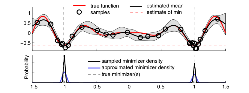
In this paper, we use a acquisition criterion that maximizes the information gain about the minimizer, or equivalently minimizes minimizer entropy (MME) [9, 10]. MME provides a balance between exploration and exploitation that is tailored specifically for finding the minimizers of global optimization problems. As a result, the MME samples densely around potential minimizers, and sparsely in the other region of the input space (Fig. 1 and 3). Furthermore, since a global map of potential minimizers is maintained, MME enables us to obtain multiple global minimizers.
2 Optimization Framework
We consider optimization target that is a continuous real-valued function , where is bounded. Furthermore, we assume has a unique minimizer (an assumption relaxed later) and that each observation is noisy; i.e. . The objective of the optimization is to find the function’s minimizer and its corresponding minimum .
The Bayesian optimization framework has been proposed to arrive to an -close solution in a sub-exponential number of function evaluations on average [2, 3, 5]. While it is possible to devise strategies seeking the jointly-optimal samples, the computational cost is often prohibitive [2, 3, 6]; hence, a greedy (or a one-step lookahead) sequential approach is typically used where the next sample is chosen according to an acquisition criterion. Popular acquisition criteria are summarized in the table below:
| Criterion | of | Description |
|---|---|---|
| Kushner [2] | Samples the point with the highest probability of lying below the current minimum estimate. | |
| Mockus [3] | Samples the point with the largest expected improvement over the current minimum estimate. |
3 Proposed Acquisition Criterion: The MME Criterion
The Bayesian framework, when applied to functional estimation, defines a prior over the functions and a corresponding posterior after observations. Statistical inference on requires the posterior . The minimizer relates deterministically to through the highly nonlinear “” operation; hence, it is intractable to compute from the posterior . In particular, consider the set of points for which the function values are close to the optimum, for a small . may not be localized even for a smooth true since the function could have multiple disjoint -close optimum regions (possibly due to multiple optimizers), making the minimizer distribution often quite complex. Therefore, in this paper, we propose utilizing the inference on as an intermediate step to learn more efficiently by focusing the sampling on the regions of that contribute the most information about the minimizer.
Let be the random variable representing the minimizer conditioned on observations. Our proposed criterion MME minimizes the minimizer entropy , where denotes the entropy functional. In this paper, we focus on a sequential sampling scheme where we seek the next point that minimizes the entropy of the minimizer given the additional sample . Thus, the next sample point is given by:
| (1) |
A straightforward evaluation of (1) requires the computation of
| (2) |
Since direct evaluation of (2) is intractable in general, we develop a more tractable approximation. In this paper, we utilize the widely used Gaussian process framework for [1, 5, 6, 11]. The minimizer’s posterior in (2) can be pointwise bounded as follows
| (3) |
where is our current estimate of the minimum. The equality results from the definition of the minimizer, while the inequality is due to the fact that implies . The upper bound in (3) is equal to where
| (4) |
where denotes normal cdf, and the posterior means, variances, and covariances can be found in [11]. Finally, we normalize and use it as a proxy .
Notice that the approximation step leads to a broader distribution with respect to the true posterior ; hence, the resulting entropy is an upper bound as well. Moreover, in the noiseless case, the two distributions converge (for functions with unique minimizer); i.e., when the posterior approaches to the true , which is a delta function at the minimizer. A natural advantage of this approximation is that it generalizes to functions with multiple global minimizers through the multi-modal (see Figure 1). However, having multiple minimizers leads to ambiguity in the posterior covariance term, , in (4). In this case, we treat and as independent and remove the covariance term from (4).
Implementation: For each sample acquisition, we have to estimate (1). This requires an expectation over for each candidate ; we use a Monte Carlo approach sampling under the prior. Given each , we use the approximation (4) and evaluate the entropy (1). This is done for each candidate on a grid, and the candidate that minimizes the criterion is chosen. An alternative to sampling , which can be costly, is to further approximate the expected posterior entropy by assuming the posterior mean function remains constant – we refer to the algorithm with this extra assumption the “fast” version.
GP requires selection of kernels and associated hyperparameters. Choosing a good hyperparameter is critical for good small sample performance, and convergence to global solution. After acquiring each sample, we use evidence optimization to infer hyperparamters (including ) [11, 12]. For the examples in the result section, we used isometric squared exponential kernel with two hyperparameters [11], and a constant mean function (1 hyperparameter).
4 Results
4.1 1D toy example
To illustrate the main ideas, we demonstrate the algorithm on a 1D function under additive Gaussian noise (Figure 1). The 1D function has two global minima and two local minima; therefore, the minimizer distribution is multi-modal. Figure 1 shows the sampling distribution of the minimizer and our approximation of it. As expected, it has two peaks corresponding to the two global minima. Furthermore, Figure 2 shows the evolution of the minimizer’s posterior and its convergence to the sharp bimodal form given in Figure 1.

4.2 2D examples
We compare our criterion against the popular criterion proposed by Mockus [3], also called Maximum Expected Improvement (MEI), on two 2D test functions with a noise variance of : Hosaki function (1 local, 1 global minimum) [4, 13], and the Dixon-Szegő 6-hump camel test function (2 local, 2 global minimum) [14]. In addition, to illustrate the effectiveness the Bayesian Optimization framework, we compare against the state-of-the-art active response surface method proposed by Krause et al. [15]. All algorithms were applied under the same prior and hyperparameter selection procedure with the only difference being the acquisition criterion. Both MEI and the response surface approach require a relatively good (initial) estimate of the hyperparameters, therefore we initialize them with random samples. Also, since the response surface method only works when the candidate set is finite, we restrict the sampling to be on a grid for all algorithms.

Fig. 3A shows the convergence for the Hosaki function in terms of median of the estimated minimum function values obtained by each method from the repetitions. Both MME and MEI performed well, while the response surface method has slower convergence and underestimates the correct minimum value due to the inaccurate estimation of . For the Dixon-Szegő test function, the MEI constantly drew samples (black dots in Fig. 3B) near one of the global minimizers, and thus failed to find the other minimum. The response surface method drew samples from all over the space and found the minimizers correctly, but the value of the minima were not as accurate. On the other hand, MME found the correct minimizers and accurate minimum values compared to the other two methods. The estimated minimum values at the global minimizers are shown in the table below.
| true | M | K | MME | |
|---|---|---|---|---|
| -0.999 | 1.185 | -1.202 | -0.960 | |
| -0.999 | -0.975 | -0.791 | -1.020 |
5 Discussion
We proposed an information theoretic active optimization criterion by focusing on learning the minimizer distribution. The problem of optimizing an unknown function is transformed to minimization of estimated entropy of minimizer obtained by Gaussian process. We plan to improve computational complexity and approximation accuracy in future work.
References
- [1] Donald R. Jones, Matthias Schonlau, and William J. Welch. Efficient global optimization of expensive Black-Box functions. Journal of Global Optimization, 13(4):455–492, December 1998.
- [2] Harold J. Kushner. A new method of locating the maximum of an arbitrary multipeak curve in the presence of noise. Journal of Basic Engineering, pages 86:97–106, March 1964.
- [3] J. Mockus. The Bayesian approach to global optimization. Lecture Notes in Control and Information Sciences, 38:473–481, 1982.
- [4] John F. Elder IV. Efficient Optimization through Response Surface Modeling: A GROPE Algorithm. PhD thesis, University of Virginia, May 1993.
- [5] Daniel J. Lizotte. Practical Bayesian optimization. PhD thesis, University of Alberta, Edmonton, Alta., Canada, 2008.
- [6] Michael A Osborne, Roman Garnett, and Stephen J Roberts. Gaussian processes for global optimization. 3rd International Conference on Learning and Intelligent Optimization (LION 3), pages 1–15, 2009.
- [7] Robert B. Gramacy and Herbert K. H. Lee. Optimization under unknown constraints. (in press), July 2010, 1004.4027.
- [8] Niranjan Srinivas, Andreas Krause, Sham Kakade, and Matthias Seeger. Gaussian process optimization in the bandit setting: No regret and experimental design. In Proc. International Conference on Machine Learning (ICML), 2010.
- [9] Julien Villemonteix, Emmanuel Vazquez, and Eric Walter. An informational approach to the global optimization of expensive-to-evaluate functions. Journal of Global Optimization, September 2008, cs/0611143.
- [10] Philipp Hennig and Christian J. Schuler. Entropy search for Information-Efficient global optimization. December 2011, arXiv:1112.1217.
- [11] Carl E. Rasmussen and Christopher K. I. Williams. Gaussian Processes for Machine Learning. The MIT Press, November 2005.
- [12] Peter Frazier, Warren Powell, and Savas Dayanik. The Knowledge-Gradient policy for correlated normal beliefs. INFORMS Journal on Computing, 21(4):599–613, 2009.
- [13] George A. Bekey and Man T. Ung. A comparative evaluation of two global search algorithms. Systems, Man and Cybernetics, IEEE Transactions on, SMC-4(1):112–116, January 1974.
- [14] L. C. W. Dixon and G. P. Szegö. The global optimization problem: an introduction. In L. C. W. Dixon and G. P. Szegö, editors, Towards Global Optimisation 2, pages 1–15. Amsterdam; New York : North-Holland Pub. Co. ; New York : Sole distributors for the U.S.A. and Canada, Elsevier North-Holland, 1978.
- [15] Andreas Krause, Ajit Singh, and Carlos Guestrin. Near-Optimal sensor placements in Gaussian processes: Theory, efficient algorithms and empirical studies. J. Mach. Learn. Res., 9:235–284, June 2008.