The Dynamics of Rayleigh-Taylor Stable and Unstable Contact Discontinuities with Anisotropic Thermal Conduction

Abstract

We study the effects of anisotropic thermal conduction along magnetic field lines on an accelerated contact discontinuity in a weakly collisional plasma. We first perform a linear stability analysis similar to that used to derive the Rayleigh-Taylor instability (RTI) dispersion relation. We find that anisotropic conduction is only important for compressible modes, as incompressible modes are isothermal. Modes grow faster in the presence of anisotropic conduction, but growth rates do not change by more than a factor of order unity. We next run fully non-linear numerical simulations of a contact discontinuity with anisotropic conduction. The non-linear evolution can be thought of as a superposition of three physical effects: temperature diffusion due to vertical conduction, the RTI, and the heat flux driven buoyancy instability (HBI). In simulations with RTI-stable contact discontinuities, the temperature discontinuity spreads due to vertical heat conduction. This occurs even for initially horizontal magnetic fields due to the initial vertical velocity perturbation and numerical mixing across the interface. The HBI slows this temperature diffusion by reorienting initially vertical magnetic field lines to a more horizontal geometry. In simulations with RTI-unstable contact discontinuities, the dynamics are initially governed by temperature diffusion, but the RTI becomes increasingly important at late times. We discuss the possible application of these results to supernova remnants, solar prominences, and cold fronts in galaxy clusters.

1 Introduction

The interface between fluids of different densities can be destabilized by gravity or other sources of acceleration. If the fluid is accelerated in a direction opposite of $\nabla\rho$, the interface is unstable to the Rayleigh-Taylor instability (RTI). When a heavy fluid is on top of a lighter fluid, the RTI is characterized by bubbles of light fluid rising into the heavy fluid, and downward spikes of heavy fluid penetrating into the light fluid (e.g., Chandrasekhar, 1961). The RTI is potentially important in a variety of astrophysical situations, e.g., in supernova remnants at the contact discontinuity between the shocked supernova gas and the shocked interstellar material (Gull, 1973; Chevalier et al., 1992; Jun & Norman, 1996); in emerging magnetic flux in the solar corona (Isobe et al., 2005; Berger et al., 2011); and in buoyant bubbles of gas produced by AGN in galaxy clusters (e.g., Robinson et al., 2004).

In some of these contexts, the plasma is hot and dilute. If the electron gyroradius is much smaller than the electron mean free path, then the heat conduction by electrons is primarily along the magnetic field (Braginskii, 1965). We will refer to this effect as anisotropic conduction. Work by, e.g., Balbus (2000), Quataert (2008), and McCourt et al. (2011), has shown that convection is strongly affected by anisotropic conduction. The normal Schwarzschild condition for convective instability, $ds/dz<0$, is modified when the conductivity time-scale is much shorter than the buoyancy time-scale. In this ‘fast conduction’ limit, plasmas are unstable to a heat flux driven buoyancy instability (HBI) when $\boldsymbol{g}\boldsymbol{\cdot}\nabla T<0$ or are unstable to the magnetothermal instability (MTI) when $\boldsymbol{g}\boldsymbol{\cdot}\nabla T>0$. Although the HBI acts to reduce the effective conductivity in the direction parallel to gravity, the MTI produces vigorous convection (e.g., Parrish & Stone, 2007; Parrish & Quataert, 2008; McCourt et al., 2011).

Our goal in this paper is to investigate the magnetized RTI when anisotropic conductivity is important. Balsara et al. (2008a) and Balsara et al. (2008b) have simulated supernova remnants with anisotropic conduction. However, their simulations are of an entire supernova remnant, and their analysis did not describe how the contact discontinuity is affected by the combination of the RTI and anisotropic conductivity. In fact, in Tilley & Balsara (2006), there does not seem to be any RTI type perturbation of the contact discontinuity, unlike in, e.g., Chevalier et al. (1992).

Our analysis will make several simplifying assumptions. We will focus our attention only on weak magnetic fields that are not dynamically important. Stone & Gardiner (2007) have shown that stronger magnetic fields prevent fluid motions which bend field lines, and that in the strong magnetic field limit, the RTI dynamics are dominated by interchange motions. Our assumption will be that the fields are strong enough to keep the conduction anisotropic, but not so large that they are dynamically important. We will also largely (though not entirely) neglect the effects of anisotropic viscosity, which acts to preferentially damp motion along magnetic fields. Previous work has shown that this also leads to the RTI being dominated by interchange motions (Dong & Stone, 2009).

In addition to studying the RTI, we will also investigate the effects of anisotropic conduction on contact discontinuities that are RTI stable. Birnboim et al. (2010) propose that cold fronts in galaxy clusters can form through the merger of shocks. These observed cold fronts are sharp contact discontinuities, and the intracluster medium (ICM) is sufficiently hot and dilute for anisotropic conduction to be important. These contact discontinuities are likely to be RTI stable, given their small widths. Parrish & Quataert (2008) and Birnboim et al. (2010) suggest that anisotropic conduction could help to maintain the small widths of cold fronts in clusters, because the HBI acts to suppress heat conduction at RTI-stable contact discontinuities.

The remainder of the paper is organized as follows. First, we perform a linear stability analysis including the effects of anisotropic conductivity on an RTI-unstable contact discontinuity with a weak horizontal magnetic field (§2). Next, we discuss our numerical methods for simulating this setup using fully non-linear compressible MHD simulations in §3. In §4 we consider the hydrodynamic problem, i.e., without magnetic fields or anisotropic conduction. Section 5 studies RTI-stable and RTI-unstable contact discontinuities, for a range of initial magnetic field orientations. Finally, in §6 we conclude and discuss the astrophysical implications of this work.

2 Linear Theory

2.1 Basic equations

Throughout this paper, we employ the same set of basic equations. They are as follows:

$$\frac{d\rho}{dt} = -\rho\nabla\boldsymbol{\cdot}\boldsymbol{v},$$ (1)

$$\rho\frac{d\boldsymbol{v}}{dt} = -\nabla p+\frac{1}{4\pi}\nabla\boldsymbol{\times}\left(\nabla\boldsymbol{\times}\boldsymbol{B}\right)-g\rho\hat{\boldsymbol{z}},$$ (2)

$$\frac{\partial\boldsymbol{B}}{\partial t} = \nabla\boldsymbol{\times}\left(\boldsymbol{v}\boldsymbol{\times}\boldsymbol{B}\right),$$ (3)

$$\rho T\frac{ds}{dt} = -\nabla\boldsymbol{\cdot}\boldsymbol{Q},$$ (4)

where $\rho$ is the density, $\boldsymbol{v}$ is the velocity, $p$ is the pressure, $\boldsymbol{B}$ is the magnetic field, $g$ is the strength of gravity, and $\hat{\boldsymbol{z}}$ is the unit vector in the $z$ direction. $T$ is the temperature, $s$ is the entropy, and $\boldsymbol{Q}$ is the heat flux given by

$$\boldsymbol{Q}=-\hat{\boldsymbol{b}}\kappa\hat{\boldsymbol{b}}\boldsymbol{\cdot}\nabla T,$$ (5)

where $\hat{\boldsymbol{b}}$ is the unit vector in the $\boldsymbol{B}$ direction, and $\kappa$ is the thermal conductivity. We also use $d/dt$ to denote the full time derivative, i.e., $d/dt=\partial/\partial t+\boldsymbol{v}\boldsymbol{\cdot}\nabla$. We will employ the thermal diffusion coefficient $\chi=T\kappa/P$ in lieu of $\kappa$. For simplicity, we will approximate $\chi$ to be constant. Throughout this paper, we will take the medium to be an ideal gas with ratio of specific heats $\gamma=5/3$, and use units where $k_{b}\mu m_{p}=1$, where $k_{b}$ is the Boltzmann constant, $\mu$ is the mean molecular weight, and $m_{p}$ is the proton mass. In these units the equation of state is $P=\rho T$, and $T$ has units of velocity squared. We will use $\delta$ to denote perturbed quantities below, i.e., $\delta\rho$ is the Eulerian perturbation of the density. In the linear problem discussed here, we will assume that the magnetic field is sufficiently weak that it is dynamically unimportant, and thus the Lorentz force can be dropped from the momentum equation. However, the Lorentz force term is kept in our non-linear simulations. In several simulations we also include effects due to anisotropic viscosity in the momentum and energy equations (see §5.4), but we do not include anisotropic viscosity in our linear analysis.

2.2 Background

We will now describe the background quantities in our linear stability problem and the properties of the perturbations. In the RTI problem, two layers of different densities and temperatures are separated by an interface at $z=0$. The pressure is taken to be continuous at the interface. We will perturb this equilibrium and investigate the linear stability of these perturbations. We restrict our attention to magnetic fields which are initially horizontal. This allows us to use a background state with a density discontinuity (and thus a temperature discontinuity) which still satisfies the energy equation (eqn. 4). To avoid any conduction within the upper and lower layers, we will assume that the background state in each layer is isothermal. This means that the background pressure and density vary as $\exp(-z/H)$ where $H$ is the density scale height. $H$ is related to $c_{s}$, the adiabatic sound speed, by $H=c_{s}^{2}/(\gamma g)$. By using isothermal domains above and below the temperature discontinuity, we can restrict our attention to instabilities caused by the discontinuity, as opposed to conduction-mediated instabilities within the upper and lower domains (e.g., the MTI or HBI). Although $\rho$ is no longer constant in the upper and lower isothermal layers, we will still refer to $\rho_{+}=\rho|_{z=+\epsilon}$ and $\rho_{-}=\rho|_{z=-\epsilon}$.

The pressure is continuous at $z=0$ so the pressure jump, $\Delta\left[P\right]$, is zero, where we define

$$\Delta\left[f\right]\equiv f|_{z=+\epsilon}-f|_{z=-\epsilon},$$ (6)

for any function $f$. This implies $\Delta\left[\rho\right]=-\Delta\left[T\right]$. The RTI corresponds to $\Delta\left[\rho\right]>0$, which yields $\Delta\left[T\right]<0$, which we would expect to also be unstable to the MTI (Balbus, 2000). However, states with $\Delta\left[\rho\right]<0$, and thus $\Delta\left[T\right]>0$, are RTI stable and we would expect to be MTI-stable as well (but for non-horizontal fields, potentially HBI-unstable). We summarize the instabilities associated with each temperature and density jump, for different initial magnetic field geometries, in Fig. 1.

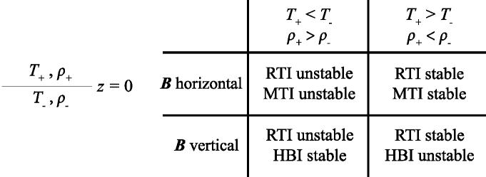
Figure 1: A schematic of the various instabilities of a contact discontinuity with anisotropic thermal conduction. On the left we show the contact discontinuity with a temperature and density of $T_{+}$ and $\rho_{+}$ immediately above the interface, and a temperature and density of $T_{-}$ and $\rho_{-}$ immediately below the interface. On the right we summarize the instabilities associated with each temperature and density jump, for either horizontal or vertical initial magnetic fields.

We assume that all perturbation quantities vary in the horizontal and time directions as

$$\delta\rho(x,y,z,t)=\delta\rho(z)\exp\left(ik_{x}x+ik_{y}y-i\omega t\right).$$ (7)

Although we Fourier decompose the perturbations in the horizontal directions, we do not Fourier decompose the perturbations in the vertical direction. We will denote by $k_{\perp}=\sqrt{k_{x}^{2}+k_{y}^{2}}$ the wavenumber perpendicular to gravity (not perpendicular to the magnetic field).

2.3 Boussinesq limit

Following e.g., Chandrasekhar (1961) or Shivamoggi (2008), we will derive the dispersion relation in two steps. First, we use the equations for the perturbations in the upper and lower layers to derive the vertical structure of the perturbations for $z\neq 0$. Second, we apply the boundary conditions. The first three are that the vertical kinetic energy decays to zero at $z\rightarrow\pm\infty$, and that the vertical velocity, $\delta v_{z}$ is continuous at $z=0$. The vertical derivative of the vertical velocity, $\partial_{z}\delta v_{z}$, is in general discontinuous at $z=0$. We thus take the limit of the equations as $z\rightarrow 0$ to derive a jump condition for $\partial_{z}\delta v_{z}$, which will lead to a dispersion relation.

First we will simultaneously employ the local and Boussinesq limits. The local limit amounts to neglecting any derivative of background quantities in the upper and lower domains in comparison to the derivative of the perturbations ($Hk_{\perp}\gg 1$). In the Boussinesq limit, $\delta P/P$ is small in comparison to e.g., $\delta\rho/\rho$. In these limits, the momentum equation (eqn. 2) gives

$$\omega^{2}\nabla^{2}\left(\rho\delta v_{z}\right)-\omega^{2}\partial_{z}\nabla\boldsymbol{\cdot}\left(\rho\delta\boldsymbol{v}\right)=k_{\perp}^{2}gi\omega\delta\rho,$$ (8)

First consider the upper and lower layers, where $z\neq 0$. One can use either the energy equation or the continuity equation to solve for $\delta\rho$. The energy equation implies

$$\left(i\omega-\omega_{c}\right)\frac{\delta\rho}{\rho}+\delta v_{z}\partial_{z}s=0,$$ (9)

where

$$\omega_{c}=\frac{2}{5}\chi k_{x}^{2}$$ (10)

is the conduction time-scale, and we take the magnetic field to be in the $\hat{\boldsymbol{x}}$ direction. The $\partial_{z}s$ term is proportional to $1/H$, which suggests it might be small in the local limit. It can be shown a posteriori that it is consistent to ignore this term (using that $Hk_{\perp}\gg 1$). When we assume that $\delta v_{z}\partial_{z}s$ is small, we get that $\delta\rho=0$ in the upper and lower layers. Then Equation 8 reduces to

$$\left(-k_{\perp}^{2}+\partial_{z}^{2}\right)\delta v_{z}=0.$$ (11)

This implies

$$\delta v_{z}\sim A_{+}\exp\left(+k_{\perp}z\right)+A_{-}\exp\left(-k_{\perp}z\right),$$ (12)

for some amplitudes $A_{+}$ and $A_{-}$. This is the same result as for the classical RTI analysis (i.e., constant density layers with no magnetic fields or conduction), so anisotropic conduction has not affected the vertical structure of the perturbations.

The next step is to apply the boundary conditions. The boundary conditions at infinity and the continuity of $\delta v_{z}$ at $z=0$ imply

$$\delta v_{z}(z)=\delta v_{z}(0)\exp\left(-k_{\perp}|z|\right),$$ (13)

where $\delta v_{z}(0)$ is an amplitude. In general we can write $\delta v_{z}\sim\exp(k_{\pm}z)$, where the plus sign is taken for $z>0$ and the minus sign is taken for $z<0$. The boundary condition at infinity requires $\mathrm{Re}(k_{+})<1/(2H)$ and $\mathrm{Re}(k_{-})>1/(2H)$. In this case, as for the classical RTI problem, we have $k_{\pm}=\mp k_{\perp}$.

Now we will discuss the jump condition on $\partial_{z}\delta v_{z}$ at $z=0$. Again we must combine the momentum equation, Equation 8, with the energy equation. The energy equation, in the limit that $z\rightarrow 0$, can be written as

$$\left(i\omega-\omega_{c}\right)\left(-i\omega\delta\rho+\delta v_{z}\partial_{z}\rho\right)=0.$$ (14)

Thus, we have that

$$-i\omega\delta\rho+\delta v_{z}\partial_{z}\rho=0$$ (15)

regardless of the value of $\omega_{c}$. This can be combined with Equations 13 and 2 to give the same dispersion relation as for the classical RTI problem,

$$\omega^{2}=\frac{gk_{\perp}\left(\rho_{-}-\rho_{+}\right)}{\rho_{+}+\rho_{-}}\equiv-Agk_{\perp},$$ (16)

where $A\equiv(\rho_{+}-\rho_{-})/(\rho_{+}+\rho_{-})$ is the Atwood number.

The key implication of Equation 16 is that in the local, Boussinesq limit the dispersion relation for the RTI is independent of the magnitude of the thermal conduction, provided that the magnetic field is aligned with the contact discontinuity. We will now briefly discuss this result. In the local limit, $d\log P/dz$ is much smaller than $k_{\perp}$, and we always have that $\Delta\left[P\right]=0$. Furthermore, the Boussinesq approximation implies that $\delta P/P\ll\delta\rho/\rho$. These facts together mean that the Lagrangian pressure perturbation, $P^{\prime}/P$ is small everywhere, where we use $f^{\prime}$ to denote the Lagrangian perturbation of $f$. The equation of state implies that

$$\frac{P^{\prime}}{P}=\frac{\rho^{\prime}}{\rho}+\frac{T^{\prime}}{T},$$ (17)

but since $P^{\prime}/P$ is small, we have that

$$\frac{T^{\prime}}{T}=-\frac{\rho^{\prime}}{\rho}=0,$$ (18)

where the last equality is due to the continuity equation (eqn. 1). This implies that in the Boussinesq approximation, perturbations are isothermal, and thus are unaffected by conduction.

The assumption that $\Delta\left[P\right]=0$ at the interface is a key part of the RTI problem. However, the assumptions that $\delta P/P$ is small and that $d\log P/dz$ is much smaller than $k_{\perp}$ result from the Boussinesq and local approximations.

2.4 Fully compressible linear theory

We will now relax the Boussinesq and local approximations and solve the linear fully compressible RTI problem including anisotropic thermal conduction. The solutions of the fully compressible equations are not isothermal, and thus are affected by anisotropic heat conduction.

As above, we must first use the evolution equations in the upper and lower layers to solve for the vertical structure of the perturbations. After some algebra, one finds the following equations for $k_{\pm}$:

$$k_{+}=\frac{1}{2H_{+}}\pm\sqrt{\frac{1}{4H_{+}^{2}}+k_{\perp}^{2}-R\frac{\omega^{2}}{gH_{+}}-\left(1-R\right)\frac{gk_{\perp}^{2}}{H_{+}\omega^{2}}},$$ (19)

$$k_{-}=\frac{1}{2H_{-}}\pm\sqrt{\frac{1}{4H_{-}^{2}}+k_{\perp}^{2}-R\frac{\omega^{2}}{gH_{-}}-\left(1-R\right)\frac{gk_{\perp}^{2}}{H_{-}\omega^{2}}},$$ (20)

where $H_{\pm}=T_{\pm}/g$ is the density scale height in the upper and lower layers, and

$$R\equiv\frac{\frac{3}{5}i\omega-\omega_{c}}{i\omega-\omega_{c}}.$$ (21)

The quantity $R$ represents the ratio of the response time-scale for pressure perturbations to the response time-scale for density perturbations. If $\omega\gg\omega_{c}$, then $R=3/5$ and perturbations are adiabatic. If $\omega_{c}\gg\omega$, then $R=1$ and perturbations are isothermal.

Note that there are two roots for each of $k_{+}$ and $k_{-}$ in Equations 19 & 20. The physical solution has perturbations with finite kinetic energy at infinity, i.e., $\mathrm{Re}(k_{+})<1/(2H_{+})$ and $\mathrm{Re}(k_{-})>1/(2H_{-})$. Since the two roots of $k_{+}$ sum to $1/(2H_{+})$ and the two roots of $k_{-}$ sum to $1/(2H_{-})$, at least one root for each of $k_{\pm}$ will be physical (Cunningham et al., 2011).

By integrating the momentum equation from $z=-\epsilon$ to $z=+\epsilon$ and dropping terms of order $\epsilon$, we derive the following dispersion relation:

$$0=gk_{\perp}^{2}\Delta\left[\rho\right]-\omega^{2}\Delta\left[\frac{\rho}{1-R\frac{\omega^{2}}{Tk_{\perp}^{2}}}\left(k_{z}-\frac{R}{H}\right)\right],$$ (22)

where $k_{z}|_{\pm\epsilon}=k_{\pm}$. Along with Equations 19 & 20, this can be used to solve for $\omega$ as a function of the various parameters of the problem – $g,k_{\perp},\omega_{c},\rho_{\pm}$ and $T_{\pm}$.

Note that for the fully compressible problem, the values of $k_{\pm}$ depend explicitly on $\omega$, so we cannot solve for the vertical structure of the perturbations before solving for the growth rate – instead we must solve for $\omega$ and $k_{\pm}$ simultaneously. Also, because the quantities inside the square roots in Equations 19 & 20 are generally complex, we do not know a priori if the square root term will have positive or negative real part. Our procedure for finding physical modes is as follows. We first pick a root for each of $k_{+}$ and $k_{-}$ and then search for an $\omega$ which satisfies the dispersion relation (eqn. 22). Then we check that for this $\omega$, $\mathrm{Re}(k_{+})<1/(2H_{+})$ and $\mathrm{Re}(k_{-})>1/(2H_{-})$. If these conditions are met, then the mode is physical.

To reduce the dimensionality of our parameter space, we nondimensionalize lengths and times by setting $k_{\perp}=2\pi$ (i.e., we set the perpendicular length scale to one) and $g=1$. We also take the smaller of $\rho_{\pm}$ to be $1$. The condition that $T_{\pm}=gH_{\pm}$ means that setting $T_{\pm}$ determines the density scale height, as well as determining the sound speed through $c_{s\pm}^{2}=\gamma T_{\pm}$. Continuity of pressure at $z=0$ requires that $T_{+}\rho_{+}=T_{-}\rho_{-}$. With all this in mind, the problem has the following degrees of freedom. First, we must pick if the top or bottom of the density discontinuity is at the lower density of $\rho=1$, as well as the density on the other side of the discontinuity (these together are equivalent to picking an Atwood number). Next, we pick the scale height on one of the sides, which uniquely sets the scale height on the other side. Finally, we must pick $\omega_{c}$.

For the unstable case, we take $\rho_{-}=1$. For simplicity, we will take $\rho_{+}=3$ ($A=1/2$), but other values of $\rho_{+}$ give qualitatively similar results. We now have only two remaining parameters: $H_{+}$ and $\omega_{c}$. In Fig. 2, we plot the growth rate, normalized to $\omega_{\mathrm{RTI}}=\sqrt{Agk_{\perp}}$ as a function of $H_{+}k_{\perp}$ for several values of $\omega_{c}/\omega_{\mathrm{RTI}}$. Without compressible effects, the growth rate would be one when normalized to $\omega_{\mathrm{RTI}}$. Note that compressibility effects become important as $c_{s}^{2}k_{\perp}^{2}$ becomes the same size as $\omega^{2}$, i.e., when $H_{+}k_{\perp}\sim 1$. Compressibility decreases the growth rate of the instability, as energy is used to compress the fluid. At large $\omega_{c}$, the perturbations are isothermal (i.e., we are in the fast conduction limit), whereas at small $\omega_{c}$, the perturbations are adiabatic.

Figure 2: Growth rates, $\omega$, normalized to $\omega_{\mathrm{RTI}}=\sqrt{Agk_{\perp}}$ as a function of $H_{+}k_{\perp}$ for various values of anisotropic thermal diffusion, parameterized by $\omega_{c}/\omega_{\mathrm{RTI}}$ (the ratio of the conduction frequency to the classical RTI growth rate). For $\omega_{c}/\omega_{\mathrm{RTI}}>10$, we are in the isothermal, or fast conduction, limit and the results are nearly equivalent to those shown for $\omega_{c}/\omega_{\mathrm{RTI}}=10$. As $H_{+}k_{\perp}$ decreases, compressibility becomes more important and $\omega/\omega_{\mathrm{RTI}}$ decreases. At a fixed $H_{+}k_{\perp}$, the growth rate increases as $\omega_{c}$ increases from zero – an asymptotic value is reached in the isothermal, or fast conduction, limit when $\omega_{c}/\omega_{\mathrm{RTI}}\gg 1$.

We will now discuss the differences between the large conductivity (isothermal, fast conduction) and small conductivity (adiabatic) limits. To make the analysis easier we will take the limit in which $H_{+}k_{\perp}$ is small. This corresponds to the limit in which the wavelength of the mode is much larger than the scale height of the background. It will turn out that $\omega^{2}/\omega_{\mathrm{RTI}}^{2}\sim H_{+}k_{\perp}$ as $H_{+}k_{\perp}\rightarrow 0$, which we will check a posteriori. First consider the isothermal limit. When $R=1$, the equations for the vertical structure (eqn. 19 & 20) become much simpler as the $1-R$ terms are zero. Given that $\omega^{2}/\omega_{\mathrm{RTI}}^{2}\sim H_{+}k_{\perp}$, the most important term in the square root when $H_{+}k_{\perp}$ is small is the $1/4H_{\pm}^{2}$ term. Thus, in this limit, $k_{+}\approx 0$ and $k_{-}\approx 1/H_{-}$.

The dispersion relation then becomes

$$\frac{-\omega^{2}}{H_{+}}\left(\frac{\rho}{1-\frac{\omega^{2}}{T_{+}k_{\perp}^{2}}}\right)=gk_{\perp}^{2}\left(\rho_{+}-\rho_{-}\right).$$ (23)

This can be easily solved to give

$$\omega^{2}=-gk_{\perp}^{2}H_{+}\frac{\rho_{+}-\rho_{-}}{\rho_{-}},\hskip 36.135pt\omega_{c}/\omega\gg 1,H_{+}k_{\perp}\ll 1.$$ (24)

We see that $\omega^{2}$ differs from $\omega_{RTI}^{2}$ by a factor of $H_{+}k_{\perp}(\rho_{+}+\rho_{-})/\rho_{-}$.

Now consider the small conductivity (adiabatic) limit. We will still take the limit in which $H_{+}k_{\perp}$ is small (i.e., the long wavelength limit). This problem is more difficult as the $1-R$ terms in Equation 19 & 20 are now important and $\omega$ appears explicitly in the formula for $k_{\pm}$. We find that

$$H_{+}k_{+} = \frac{1}{2}-\sqrt{\frac{1}{4}-\frac{2}{5}\frac{1}{\overline{\omega^{2}}}},$$ (25)

$$H_{-}k_{-} = \frac{1}{2}+\sqrt{\frac{1}{4}-\frac{2}{5}\frac{1}{\overline{\omega^{2}}}\frac{\rho_{+}}{\rho_{-}}},$$ (26)

where $\overline{\omega^{2}}=\omega^{2}/(H_{+}^{2}k_{\perp}^{2})$ is a normalized growth rate. The dispersion relation can then be written as

$$\overline{\omega^{2}}\left[\left(1-\frac{3}{5}\overline{\omega^{2}}\frac{\rho_{-}}{\rho_{+}}\right)\left(H_{+}k_{+}-\frac{3}{5}\right)\right.$$ (27)

$$-\left.\left(1-\frac{3}{5}\overline{\omega^{2}}\right)\left(\frac{\rho_{-}}{\rho_{+}}\right)^{2}\left(H_{-}k_{-}-\frac{3}{5}\right)\right]$$

$$= \left(1-\frac{\rho_{-}}{\rho_{+}}\right)\left(1-\frac{3}{5}\overline{\omega^{2}}\frac{\rho_{-}}{\rho_{+}}\right)\left(1-\frac{3}{5}\overline{\omega^{2}}\right).$$

This is an equation for $\overline{\omega^{2}}$ with only one free parameter, $\rho_{-}/\rho_{+}$. We were unable to find a general analytic solution for arbitrary values of $\rho_{-}/\rho_{+}$. However, the equation can easily be solved numerically. For $\rho_{-}/\rho_{+}=1/3$ or $A=1/2$, we have that $\overline{\omega^{2}}\approx-0.992$. Note that for the isothermal calculation, when $\rho_{-}/\rho_{+}=1/3$ or $A=1/2$ we have $\overline{\omega^{2}}=-2$.

We generally find that the growth rate for isothermal perturbations is faster than for adiabatic perturbations. This can be explained by describing how isothermal and adiabatic perturbations move in an isothermal atmosphere. The ratio of densities between a perturbed fluid element and its surroundings remains constant if the perturbation and background are isothermal. However, for adiabatic perturbations, the density of an upward propagating (low density) perturbation drops less quickly than the density of the background, so the perturbed element is less buoyant as it rises. Similarly, an adiabatically falling (high density) perturbation increases in density less quickly than the background, so the perturbed element feels a smaller downwards gravitational force as it falls.

Increasing the anisotropic conductivity from zero to infinity, the value of the $R$ parameter moves from one to $3/5$ through the complex plane. We have not found any overstabilities in this problem. The behavior at low $H_{+}k_{\perp}$ is given by Equations 25-27, replacing $2/5$ by $1-R$ and $3/5$ by $R$. The growth rate increases smoothly from the adiabatic value to the isothermal value as $\omega_{c}$ increases. Most of the change in $\omega$ as $\omega_{c}$ varies occurs when $\omega_{c}$ is near the adiabatic and isothermal growth rates.

The most prominent feature of the growth rates as $H_{+}k_{\perp}$ becomes small (i.e., for long wavelength modes) is that the growth rates also become very small. One possible interpretation is that these modes are very compressible and most of the potential energy gained by changing vertical position is absorbed by compression. A different interpretation involves the background density profile. Assume that a mode of wavelength $k_{\perp}$ is ‘sensitive’ to a distance about $1/k_{\perp}$ above and below the interface. If $H_{+}k_{\perp}\gg 1$, then the density is almost constant above and below the interface. However, if $H_{+}k_{\perp}\ll 1$, there are many density scale heights that can fit within a length $\sim 1/k_{\perp}$. In this limit, the density jump at $z=0$ looks like a small perturbation to an almost isothermal atmosphere. In this situation the RTI is relatively insignificant because the density jump is small compared to the isothermal stratification, so the growth rate should also be small.

3 Numerical Methods

We will now discuss the evolution of the RTI in the non-linear regime. We will first discuss our numerical methods, and then review and clarify previous results on the hydrodynamic RTI. We then run simulations of the RTI problem with conduction, with various magnetic field geometries. We will primarily be tracking the non-linear evolution by measuring the height of the highest buoyant bubble as a function of time.

We perform fully non-linear simulations using the Athena code (Gardiner & Stone, 2008; Stone et al., 2008), which solves the compressible evolution equations in conservative form using a Godunov method. We implement anisotropic conductivity as described in Parrish & Stone (2005) and Sharma & Hammett (2007).

The simulation domain is Cartesian, with the computational domain $x,y\in[-L/2,+L/2]$, $z\in[-L,+L]$ for some box length $L$. We normalize our lengths to $L$ (i.e., set $L=1$) in all our simulations. Simulations are run at three resolutions: 64x64x128, 128x128x256, and 256x256x512. The boundary conditions are periodic in the horizontal directions. At the top and bottom boundaries, the pressure is extrapolated to maintain hydrostatic equilibrium, and reflecting boundary conditions are applied to the remaining variables.

Our initial conditions for temperature are $T=T_{+}$ for $z>0$ and $T=T_{-}$ for $z<0$. The pressure and density, within the isothermal domains, are given by

$$P_{\pm}(z),\rho_{\pm}(z)\sim\exp(-gz/T_{\pm}),$$ (28)

so the scale height within the domains is $H_{\pm}=T_{\pm}/g$. We will refer to $\rho_{\pm}=\rho|_{\pm\epsilon}$. In all of our simulations we take the smaller of $\rho_{\pm}$ to be one and the larger to be three. The ratio $H_{\pm}/L$ relates the sound crossing time of the box to the RTI growth time for perturbations with wavelengths comparable to the size of the box. In all of our simulations, we pick $H/L=100$ and $g=1$, where $H$ is the scale height on the $\rho=1$ side of the interface. We take $\gamma=5/3$, so $c_{s}^{2}=\gamma T=500/3$ on the side of the interface with $\rho=1$. The sound crossing time is $\approx 13$, in comparison to the RTI growth time for modes the size of the box, $\approx 1.7$. Thus, our simulations are fairly incompressible.

The uniform magnetic field is taken to be horizontal, vertical, or forming a 45 degree angle with the horizontal. The magnetic field strength is set to $B/\sqrt{4\pi}=0.0001$. For the linear RTI, such a field would produce noticeable dynamical effects only on length scales comparable to $5\times 10^{-7}$ (Stone & Gardiner, 2007, hereafter SG07), which cannot be resolved by our simulations. Furthermore, the Alfvén velocity is about $10^{-5}c_{s}$. Thus, the magnetic field plays no dynamical role.

The conductivity, $\chi$, is normalized to $\sqrt{gL^{3}}$. That is, if we take $\omega_{RTI}=\sqrt{2\pi Ag/L}$ and $\omega_{c}=\frac{2}{5}\chi 4\pi^{2}/L^{2}$, where $L$ is the length of the box, then $\omega_{c}/\omega_{RTI}=2(2\pi)^{1.5}/(5\sqrt{A})\chi\approx 9\chi$ for our problem. We will primarily pick values of $\chi$ smaller than one to understand the interaction of conductivity with the RTI.

We start the simulations with a small perturbation to the vertical velocity. We set the velocity to $A_{0}R(1+\cos(\pi z/L))$, where $A_{0}$ the amplitude and $R$ is a random number between $-1$ and $+1$, as in SG07. The $z$ dependence is chosen so there is no vertical perturbation at the top and bottom boundaries. We take $A_{0}=0.05$, which implies that the maximal velocity perturbations (of size $2A_{0}=0.1$) are $\sim 0.01c_{s}$. The initial perturbations are large enough to start the simulations close to the non-linear regime. In Appendix A we discuss simulations with smaller initial perturbations which probe the linear regime discussed in §2.

4 RTI Without Conductivity

Before presenting the results of our simulations, we briefly discuss previous results on the non-linear evolution of the RTI as presented in Dimonte et al. (2004). Non-linear effects become important for perturbations of wavelength $\lambda=2\pi/k$ when the perturbation has moved the interface a height $\sim\lambda$ up or down. The ascending light fluid is described as a bubble, whereas the descending heavy fluid is described as a spike. The main diagnostic we will use is the height of the highest bubble as a function of time. The results for the depth of the lowest spike as a function of time are qualitatively similar. In laboratory experiments and numerical simulations, the height $h$ is reported to grow as

$$h=\alpha_{h}Agt^{2},$$ (29)

where $A$ is the Atwood number and $\alpha_{h}\approx$0.04–0.08 is a dimensionless number arrived at experimentally. Numerical simulations produce values of $\alpha_{h}$ around a factor of two lower than physical experiments – this is thought to be due to increased diffusion at the interface in numerical simulations (Dimonte et al., 2004).

Table 1: Parameters for simulations without conductivity.

Name	Resolution	Constant $\rho$ or $T$
SG	256x256x512	$\rho$
RTLR	64x64x128	$T$
RT	128x128x256	$T$
RTHR	256x256x512	$T$

The simulations have either constant $\rho$ layers, as in SG07, or constant $T$ layers. The simulation with constant $\rho$ layers is run using the same parameters as the hydrodynamic run in SG07. These parameters are described at the beginning of §4. The simulations with constant $T$ layers are run as described in §3.

To provide some context for the calculations with anisotropic conduction to follow, we now make a detailed comparison with the hydrodynamic RTI simulation of SG07. We have run a numerical simulation using the exact same parameters as reported in SG07.We compare this to a simulation using the initial conditions described in §3 that we will use for our simulations with anisotropic thermal conduction.

In previous work on the RTI with constant density layers, the height of the highest bubble is typically defined using the fraction of heavy fluid ($f_{h}$) and the fraction of light fluid $(f_{l}=1-f_{h})$ within a volume (Dimonte et al., 2004). If we use $\rho_{+}/\rho_{-}=3$, then $\rho=2f_{h}+1$. At $t=0$, $f_{h}=1$ above the temperature discontinuity. Thus, many define the height of the highest bubble to be the highest point at which the horizontally averaged $f_{h}$ deviates from one by a small amount. We will denote horizontal averages of quantities using $\langle\cdot\rangle$, e.g., the horizontal average of $f_{h}$ is $\langle f_{h}\rangle$. In SG07, the height is defined to be the highest point at which $\langle f_{h}\rangle$ is less than 0.985. This corresponds to the highest point at which the density is less than $\rho=2.97$. Using a lower cutoff density (or equivalently, a smaller value of $f_{h}$) does not qualitatively change our results.

In Table 1 we list our simulations which have no conductivity. In run SG we use the parameters reported in SG07. In the simulations beginning with RT, we use the initial conditions described in §3. We use the suffix LR to denote low resolution runs with resolutions of 64x64x128 and HR to denote high resolution runs with resolutions of 256x256x512. RT is our fiducial model which we will compare to our simulations with anisotropic conduction.

In the runs labelled RT and the simulations with anisotropic conduction presented in §5, the density is a function of height, but the temperature is initially constant in the upper and lower layers. Thus, we will define the height to be the highest point at which $\langle T\rangle$ differs from $T_{+}$ by more than 1 per cent. This is equivalent to the definition of height used by SG07 provided that the pressure does not change significantly through the simulation. In run SG, we use the same definition of height as SG07.

We plot the height for runs SG (using the same parameters as SG07) and RTHR (our high resolution simulation without conduction) in the top panel of Fig. 3. The two simulations give similar results. Interestingly, they both differ somewhat from the data in SG07 (their fig. 8). It is unexpected that run SG has a different height than the corresponding simulation in SG07, as we have used the exact same parameters and a newer version of the same code as reported in SG07. Nevertheless, our results are qualitatively similar. The differences between our results and those of SG07 are presumably due to a small difference in initial conditions or parameters of the run that we have not been able to identify.

Figure 3: The height of the highest bubble (defined in §4) as a function of time in RTI simulations without conduction. In the top panel the height is plotted against $t^{2}$. In the bottom panel the height is plotted on a log-log plot against $t$. We show the results from our high resolution simulation without conduction (solid line; RTHR in Table 1) and our simulation using the parameters of SG07 (dashed line; SG). The two dotted lines show power law relations with exponents of one and two. Although the height vs. $t^{2}$ line in the upper panel might look fairly linear, the bottom panel shows that the height grows linearly with $t$ at later times.

In the upper panel of Fig. 3 we plot $h/L$ as a function of $Agt^{2}/L$, as is often done in the literature (e.g., Dimonte et al., 2004). We expect to have $h=\alpha_{h}Agt^{2}$, so we expect a straight line in this figure. Near $t=0$, the slope is changing rapidly, but the lines are fairly linear at later times. However, it is very difficult to tell from a plot of $h$ vs. $t^{2}$ whether or not the height is truly increasing as $t^{2}$.

To test whether $h$ is in fact increasing as $t^{2}$, we plot $h$ vs. $t$ on a log-log plot in the bottom panel of Fig. 3. The dotted lines show power laws with exponents of one and two. Although the two simulations are initially roughly consistent with $h\sim t^{2}$, for times past $t/\sqrt{L/Ag}\approx 1.3$, the results are more consistent with the height increasing linearly with time. The numerical results from SG07 are also consistent with the height increasing linearly with time.

In Fig. 4 we plot, for three different resolutions, the height normalized to $L$ as a function of $Agt^{2}$ normalized to $L$. There is no significant agreement between the simulations at different resolutions. However, in the bottom panel of Fig. 4, we show the height normalized to $D_{\mathrm{dom}}$ as a function of $Agt^{2}$ normalized to $D_{\mathrm{dom}}$, where $D_{\mathrm{dom}}$ is the size of the first dominant bubbles and spikes in each simulation. There is much closer agreement between the runs at different resolutions using this normalization. This effect was previously noted by, e.g., Dimonte et al. (2004).

The statement that $h$ should increase as $t^{2}$ is often motivated by dimensional analysis: if the only dimensional parameter in the problem is $g$, then we must have that $h=Cgt^{2}$ for some dimensionless coefficient $C$ (which is related to the Atwood number). However, our simulations show there is another dimensional number in the problem: $D_{\mathrm{dom}}$. When we increase the resolution of our simulations by a factor of two in each direction, $D_{\mathrm{dom}}$ decreases by a factor of about two. The bottom panel of Fig. 4 shows that the relevant length scale for the non-linear evolution is $D_{\mathrm{dom}}$, and indicates that the simulations remember the size of the initial dominant modes very late into the non-linear regime.

Figure 4: The height of the highest bubble (defined in §4) as a function of time for our RTI simulations without conduction at different resolutions. In the upper panel the height and $Agt^{2}$ are normalized by the length of the box $L$. In the lower panel, the height and $Agt^{2}$ are normalized by $D_{\mathrm{dom}}$, the size of the first dominant bubbles. We plot our results for our low resolution run (solid line; RTLR in Table 1), our fudicual run (dashed line; RT), and our high resolution run (dot-dashed line; RTHR). We estimate $D_{\mathrm{dom}}$ to be $L/32$, or about 8 cell widths for our high resolution simulation. We then take $D_{\mathrm{dom}}=L/16$ and $L/8$ for our fiducial simulation and low resolution simulation respectively. The results line up well when normalizing lengths to $D_{\mathrm{dom}}$, but there is little agreement between the different resolutions when normalizing lengths to $L$. This indicates that the simulations do not notice the size of the box, but instead remember the size of the first dominant modes. The flat portion of the curves correspond to when the perturbations have hit the top of the box in each of the simulations.

With another dimensional number in the problem, $D_{\mathrm{dom}}$, we can make a new dimensionless parameter, $D_{\mathrm{dom}}/(gt^{2})$. With this additional dimensionless parameter, the height is no longer required to increase as $gt^{2}$. Instead, for instance, the height could increase as $t\sqrt{D_{\mathrm{dom}}g}$. Physically, this would correspond to a bubble of fixed size rising at its terminal velocity. This functional form fits our numerical results, although the size of the bubbles in our simulation increase as a function of time (see Fig. 5).

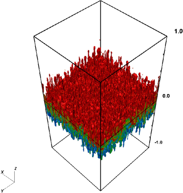
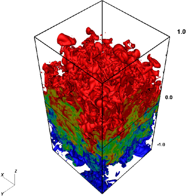
Figure 5: Isosurfaces of temperature at $T=95$ and $T=38$ for the high resolution simulation without any explicit conductivity (RTHR in Table 1). The upper (lower) layer is initialized with a temperature of 33 (100). The upper panel is at time $t/\sqrt{L/Ag}\approx 1.8$, and the lower panel is at time $t/\sqrt{L/Ag}\approx 4.2$. Temperature contours are also shown on the faces of the simulation domain. The height of the highest bubble is increasing linearly at both times shown (see Fig. 3), consistent with a bubble of fixed size rising at its terminal velocity. However, the size of the bubbles is increasing, which would yield larger terminal velocities at later times.

Although we do not have a satisfactory explanation for why the height increases linearly with time, it is clear that our results are not consistent with the commonly repeated result that the height increases quadratically with time. We have also shown that the results of SG07 are also not consistent with the height increasing quadratically with time (although SG07 did not make this point explicitly). This shows that care must be taken when determining the functional form of $h(t)$.

With this in mind, we will now include anisotropic conductivity in our calculations. We will be making frequent comparison with our fiducial RTI simulation without explicit conduction (RT in Table 1), as well as with the results shown in Figures 3–5.

5 Results with Anisotropic Conduction

Anisotropic conduction enables diffusive spreading of the initial temperature discontinuity. Even horizontal fields induce diffusive spreading – the small $v_{z}$ from the initial perturbation produces a small vertical field component. This produces a small amount of perpendicular temperature diffusion when the interface between the two constant temperature layers is within a cell. To distinguish mixing of temperature from mixing of material on either side of the interface, we will introduce two new definitions of height. We will call the definition used in §4 the height of the temperature mixing layer, or $h_{T}$. As before, it is defined to be the highest point at which $\langle T\rangle$ differs from $T_{+}$ by more than 1 per cent. We will also sometimes calculate the depth of the temperature mixing layer, or $d_{T}$. Similarly, $d_{T}$ is the lowest point at which $\langle T\rangle$ differs from $T_{-}$ by more than 1 per cent.

In addition, we initialize the simulations with two passive scalar fields which we will call $C_{L}$ and $C_{U}$. The simulations start with $C_{L}=1$, $C_{U}=0$ for $z<0$ and with $C_{L}=0$, $C_{U}=1$ for $z>0$. We define the two heights of the composition mixing layer, $h_{C_{L}}$ and $h_{C_{U}}$, to be the highest points for which $\langle C_{L}\rangle$ or $\langle C_{U}\rangle$ differ from their initial value by more than 0.015. That is, $h_{C_{L}}$ is the highest point at which $\langle C_{L}\rangle>0.015$ and $h_{C_{U}}$ is the highest point at which $\langle C_{U}\rangle<0.985$. When there is no temperature diffusion, $h_{T}=h_{C_{L}}=h_{C_{U}}$ provided that $\rho_{+}=3$ and $\rho_{-}=1$, so the height of the temperature mixing layer, the two heights of the composition mixing layer, and the height of the highest RTI bubble all coincide.

In Table 2 we list the simulations with conduction that we will discuss in this paper. We studied interfaces with RTI-stable or RTI-unstable jumps in temperature, as well as magnetic fields which are initially horizontal, vertical, or at a 45 degree angle to the horizontal (see Fig. 1). The names of simulations with initially horizontal magnetic fields start with ‘H’ in Table 2, whereas the names of simulations with initially vertical magnetic fields start with ‘V.’ The two simulations with an initial magnetic field at a 45 degree angle to the horizontal have names starting with ‘A.’ Simulations which are RTI stable have an ‘S’ as the second character in their name. We vary the thermal diffusivity, which is given by $\chi=10^{-n}$, where $n$ is the number in the name of the simulation (in simulations with initially skewed magnetic fields, $\chi=2\times 10^{-n}$). A diffusivity of $10^{-n}$ corresponds to $\omega_{c}/\omega_{\mathrm{RTI}}=9\times 10^{-n}$, where $\omega_{c}$ is conduction frequency over the simulation domain, and $\omega_{\mathrm{RTI}}$ is the RTI growth rate for modes the scale of the simulation domain. Some of our simulations employ isotropic instead of anisotropic conduction – these have the letter ‘I’ in their names. Most of our simulations are at a resolution of 128x128x256 (the simulations with RTI-stable temperature jumps and vertical magnetic field are run for longer, so they use a resolution of 64x64x128). However, to test resolution effects, we ran some simulations at a resolution of 256x256x512 (we ran the simulations with RTI-stable temperature jumps with vertical magnetic fields at a resolution of 128x128x256) – these high resolution runs are denoted by ‘HR.’

Table 2: Parameters for simulations with conductivity.

Name	Resolution	$\omega_{c}/\omega_{\mathrm{RTI}}$	$\boldsymbol{B}$ dir.	RTI stability
H0	128x128x256	9	hor.	unstable
H1	128x128x256	0.9	hor.	unstable
H2	128x128x256	0.09	hor.	unstable
H2HR	256x256x512	0.09	hor.	unstable
HS0	128x128x256	9	hor.	stable
HS1	128x128x256	0.9	hor.	stable
HS2	128x128x256	0.09	hor.	stable
HS2HR	256x256x512	0.09	hor.	stable
V1	128x128x256	0.9	ver.	unstable
V2	128x128x256	0.09	ver.	unstable
V3	128x128x256	0.009	ver.	unstable
V3HR	256x256x512	0.009	ver.	unstable
VS2	64x64x128	0.09	ver.	stable
VS3	64x64x128	0.009	ver.	stable
VS3HR	128x128x256	0.009	ver.	stable
VS4	64x64x128	0.0009	ver.	stable
VS1I	128x128x256	0.9 (i)	ver.	stable
VS2I	128x128x256	0.09 (i)	ver.	stable
VS3I	64x64x128	0.009 (i)	ver.	stable
VS3IHR	128x128x256	0.009 (i)	ver.	stable
VS4I	128x128x256	0.0009 (i)	ver.	stable
A3	128x128x256	0.018	$45^{\circ}$	unstable
AS2	128x128x256	0.18	$45^{\circ}$	stable

The simulations are run as described in §3. The conductivity is anisotropic except for the simulations labelled (i). $\omega_{c}$ is the conduction time-scale across the simulation domain and $\omega_{\mathrm{RTI}}$ is the RTI growth rate for modes with wavelengths comparable to the size of the simulation domain. If the simulation is listed as RTI-unstable, then $\rho_{+}=3$ and $\rho_{-}=1$. If the simulation is listed as RTI-stable then $\rho_{+}=1$ and $\rho_{-}=3$.

5.1 Horizontal magnetic field

Systems with horizontal magnetic fields and anisotropic conduction are sometimes susceptible to the MTI. The MTI and RTI both occur when $\rho_{+}>\rho_{-}$. We will start by discussing the case where $\rho_{+}<\rho_{-}$. There is neither MTI nor RTI in this case, so the dynamics are dominated by diffusion perpendicular to the magnetic field lines due to a combination of small perturbations to the field orientation and numerical mixing across the interface. If a simulation is run with no initial perturbation, we find that the code holds the equilibrium exactly.

5.1.1 RTI-stable and MTI-stable ($\rho_{+}<\rho_{-}$)

Because there is neither MTI nor RTI the distinction between the height of the temperature mixing layer ($h_{T}$) and the composition mixing layer ($h_{C_{L}}$ and $h_{C_{U}}$) is very important. In Fig. 6 we plot $\langle T\rangle$, $\langle C_{L}\rangle$, and $\langle C_{U}\rangle$ as a function of $z$ at $t/\sqrt{L/Ag}\approx 3.5$ for our high resolution run with $\omega_{c}/\omega_{\mathrm{RTI}}=0.09$ (HS2HR in Table 2). Several effects can be seen in this figure. First, the vertical position of the interface (about where $\langle C_{L}\rangle$ and $\langle C_{U}\rangle$ intersect) is above $z=0$. Because the interface is moved upwards, the upper layer is compressed, causing $C_{U}$ to build up above the interface. Note that there is very little movement of material across the interface – the gradient of $\langle C_{U}\rangle$ remains large throughout the simulation. Similarly, $\langle C_{L}\rangle$ does not spread upwards across the interface. However, because the interface is moving upwards, $C_{L}$ is spreading out below the interface. In fact, the depth associated with $\langle C_{L}\rangle$ is equal to the depth associated with $\langle T\rangle$. Also notice that our metrics for the height of the composition mixing layer are sensitive to both the width of the composition mixing layer and the vertical position of the centre of the mixing layer. Thus, the size of the mixing layer is actually being overestimated by $h_{C_{L}}$ and $h_{C_{U}}$, despite remaining small throughout the simulations. The results depicted in Fig. 6 are similar for other times – at earlier times, the interface is closer to $z=0$, whereas at later times, the interface is at a higher vertical position.

The origin of the upwards motion of the interface can be understood as follows. Because of the small initial perturbation to $v_{z}$ and numerical mixing across the interface, there is some vertical conduction of heat. The perpendicular conduction is proportional to the amplitude of the initial perturbation which adds a small vertical component to the magnetic field. This vertical heat conduction will produce a vertical pressure force in the following manner. Consider the dynamics at the beginning of the simulation and very close to the interface at $z=0$. Initially the temperature above the interface is higher than the temperature below the interface, while the pressure is about equal above and below the interface. Dynamically nothing is happening because the interface is stable to dynamical perturbations. However, there is some vertical heat conduction, so on a temperature diffusion time-scale, heat is transferred from above the interface to below the interface. Since the temperature above the interface drops, the pressure above the interface also drops. Similarly, the pressure below the interface increases. This pressure difference pushes the interface upwards.

Figure 6: Profiles of $\langle T\rangle$, $\langle C_{L}\rangle$ and $\langle C_{U}\rangle$ for our high resolution RTI-stable simulation with $\omega_{c}/\omega_{\mathrm{RTI}}=0.09$ (HS2HR in Table 2) at $t/\sqrt{L/Ag}\approx 3.5$. $C_{L}$ ($C_{U}$) is a passive scalar initialized to one (zero) for $z<0$ and zero (one) for $z>0$ which track the mixing of density, rather than the mixing of temperature (which is affected by heat diffusion). The vertical dotted line is at $z=0$. The interface (about where $\langle C_{L}\rangle=\langle C_{U}\rangle$) has moved upwards from $z=0$, compressing $C_{U}$ above the interface and spreading out $C_{L}$ below the interface. This upwards motion is due to a pressure force caused by the small vertical heat diffusion in the simulation.

In Fig. 7 we plot the height as a function of time for several different values of $\omega_{c}/\omega_{\mathrm{RTI}}$. $h_{C_{L}}$ and $h_{C_{U}}$ are only plotted for the high resolution simulation (HS2HR in Table 2), but these heights are similar for the other simulations. As the conductivity increases, all the height metrics increase, although $h_{C_{L}}$ and $h_{C_{U}}$ remain about an order of magnitude smaller than $h_{T}$. Note that $h_{T}$ is slightly larger at higher resolutions. This might be because the upwards pressure force due to conduction is larger for smaller cell widths, as the initial gradient is sharper. We have defined $h_{C_{L}}$ and $h_{C_{U}}$ to be the points at which $\langle C_{L}\rangle$ and $\langle C_{U}\rangle$ differ by 1.5%, which corresponds to a 1 per cent temperature variation if $\rho_{+}=3$. However, in these simulations $\rho_{+}=1$, so if $T,C_{L},$ and $C_{U}$ were all mixed by the same amount, we would expect $h_{C_{L}}=h_{C_{U}}$ to be larger than $h_{T}$, instead of much smaller than $h_{T}$ as shown in Fig. 7. This highlights the fact that the dominant effect in these RTI-stable simulations is simple temperature diffusion which increases $h_{T}$ much more than $h_{C_{L}}$ or $h_{C_{U}}$.

Figure 7: Heights (defined in §5) as a function of time for various simulations with horizontal magnetic fields and an RTI-stable temperature jump. The solid and dotted lines are plots of $h_{T}$, the height of the temperature mixing layer. The highest solid line correspond to the run with $\omega_{c}/\omega_{\mathrm{RTI}}=9$ (HS0 in Table 2), the middle solid line correspond to the run with with $\omega_{c}/\omega_{\mathrm{RTI}}=0.9$ (HS1), and the lowest solid line and dotted line correspond to the two runs with $\omega_{c}/\omega_{\mathrm{RTI}}=0.09$ (solid line is at the fiducial resolution, HS2; dotted line is the high resolution run, HS2HR). The dashed and dot-dashed lines show $h_{C_{L}}$ and $h_{C_{U}}$ respectively for simulation HS2HR; these are two metrics for the height of the composition mixing layer. If there was no perpendicular temperature diffusion, all heights would stay at zero for the entire simulation. Although little material diffuses across the interface, $h_{C_{L}}$ and $h_{C_{U}}$ increase slowly due to a pressure force which raises the interface.

We also tracked the amplification of magnetic energy in the simulations. The results are shown in Fig. 8. In this figure, we plot the growth of magnetic energy for all our high resolution simulations. For comparison, we include the high resolution simulation without any explicit conductivity (solid line). In the RTI-unstable simulation without any explicit conductivity, the magnetic energy grows exponentially for most of the simulation. This is because the magnetic field remains dynamically unimportant for the entire simulation. In our high resolution RTI-stable simulation with a horizontal initial magnetic field, there is some initial linear growth in the magnetic energy which saturates by $t/\sqrt{L/Ag}\approx 2$; the magnetic energy increases by a factor of four. This is likely due to the initial velocity perturbation. Unsurprisingly, the growth is significantly smaller than in the RTI-unstable simulation, although the two cases have the same initial magnetic field.

Figure 8: The magnetic energy, $|\boldsymbol{B}|^{2}/8\pi$, normalized to the initial magnetic energy as a function of time. We show results from our high resolution simulation without any explicit conductivity (solid line; RTHR in Table 1); our high resolution simulations with initially horizontal magnetic fields with $\omega_{c}/\omega_{\mathrm{RTI}}=0.09$, one which is RTI-stable (dotted line; HS2HR in Table 2), the other which is RTI-unstable (dashed line; H2HR); and our high resolution simulations with initially vertical magnetic fields with $\omega_{c}/\omega_{\mathrm{RTI}}=0.009$, one which is RTI-stable (triple-dot-dashed line; VS2HR), and one which is RTI-unstable (dot-dashed line; V2HR). The HBI-unstable simulation, VS2HR, is run for much longer than the other simulations; for convenience, we rescale the time variable using a scaling factor $S$ which is equal to 12 for simulation VS2HR and 1 for all other simulations. The RTI-unstable simulations exhibit exponentially growing magnetic energies, whereas the RTI-stable simulations show linearly increasing magnetic energies.

These results highlight the essential role of perpendicular thermal conduction in our RTI-stable simulations with horizontal magnetic fields. Without the perpendicular conduction, there would be no vertical temperature diffusion, so $h_{T}$ would stay close to zero for the entire simulation. The interface would also not rise so $h_{C_{L}}$ and $h_{C_{U}}$ would also stay close to zero. In any astrophysical context, however, there will always be some diffusion across the interface. Temperature diffusion across the interface could occur due to some small perpendicular diffusion, or because the magnetic field is not completely parallel to the interface. In these cases the system will evolve as shown in Figures 6 & 7, although the time scale for diffusion will depend on the source and strength of diffusion across the interface.

5.1.2 RTI-unstable and MTI-unstable ($\rho_{+}>\rho_{-}$)

When the density above the interface is larger than the density below it, the contact discontinuity is RTI-unstable. We plot $h_{T}$ for the RTI-unstable simulations for several values of $\omega_{c}/\omega_{\mathrm{RTI}}$ as solid lines in Fig. 9. We also plot the depth of the temperature mixing layer, $d_{T}$, for the RTI-stable simulations for several values of $\omega_{c}/\omega_{\mathrm{RTI}}$ as dashed lines. Using these two sets of lines, we can determine when the increase in height is due to vertical heat conduction and when it is due to RTI non-linear mixing. Both the depth of the temperature mixing layer in the RTI-stable case and the height of the temperature mixing layer in the RTI-unstable case describe how temperature penetrates into the layer with $T=100/3$. If vertical heat conduction is more important than the RTI, then we would expect $h_{T}$ for the RTI-unstable case to equal $-d_{T}$ for the RTI-stable case. Indeed, we see that $h_{T}$ is very close to $-d_{T}$ for the entire simulation when $\omega_{c}/\omega_{\mathrm{RTI}}=9$ and $0.9$. This indicates that vertical heat conduction dominates the RTI for these diffusivities. However, when $\omega_{c}/\omega_{\mathrm{RTI}}=0.09$, the vertical heat conduction only dominates until $t/\sqrt{L/Ag}\approx 1-2$. After this time, the RTI becomes more important, and the height increases as in our fiducial simulation with no explicit conduction.

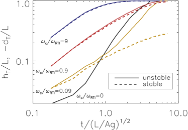
Figure 9: Heights and depths of the temperature mixing layer (defined in §5) as a function of time for various $\omega_{c}/\omega_{\mathrm{RTI}}$ for simulations with horizontal initial magnetic fields. The solid lines show $h_{T}$ for our simulations which are RTI-unstable, whereas the dotted lines show $-d_{T}$ for our simulations which are RTI-stable. The top pair of blue lines, which are almost overlapping are for $\omega_{c}/\omega_{\mathrm{RTI}}=9$ (H0 and HS0 in Table 2). Below these, the red pair of lines, which are also almost overlapping are for $\omega_{c}/\omega_{\mathrm{RTI}}=0.9$ (H1 and HS1). The lowest pair of lines, which are in yellow, correspond to $\omega_{c}/\omega_{\mathrm{RTI}}=0.09$ (H2 and HS2). The bottom solid line shows $h_{T}$ for our fiducial simulation without explicit conductivity (RT in Table 1). The height for the RTI-unstable runs is about equal to the depth for the RTI-stable runs when conduction dominates over the RTI, which is for most of the simulation when $\omega_{c}/\omega_{\mathrm{RTI}}=9$ and $0.9$. However, for $\omega_{c}/\omega_{\mathrm{RTI}}=0.09$, the RTI becomes important around $t/\sqrt{L/Ag}\approx 1-2$, and the height in the RTI-unstable simulation increases in a similar way to the height in the simulation without conductivity. The results are qualitatively similar at higher resolution.

In general, vertical heat conduction is always faster than the RTI early in the simulation because the conduction time over the length scale associated with the discontinuity is nearly zero. Thus, the temperature is essentially unaffected by the RTI at early times. However, the RTI does continue to grow, even in the diffusion-dominated regime early in the simulations. The RTI bubbles grow faster than heat diffuses, so the RTI always wins at late times provided the simulation domain is large enough. The transition to the RTI-dominated regime occurs when the height of the RTI bubbles reaches the height of the temperature mixing layer due to conduction alone. If the RTI was occurring independently of the conduction, this would occur when $h_{T}$ in our fiducial simulation equals $-d_{T}$ for the RTI-stable case. This is broadly in agreement with Fig. 9.

However, the height after the transition to the RTI-dominated regime is not equal to the height in our fiducial simulation which has no explicit conductivity. The simulations with anisotropic conduction are more dissipative so the height increases more slowly than when there is no explicit conductivity. This is the principal effect of anisotropic conduction for the horizontal field, RTI-unstable case, in the RTI-dominated regime. The increase in dissipation is due to magnetic field lines penetrating the bubbles and diffusing their temperature into the surrounding medium. This decreases the buoyancy of the bubbles and slows their rise.

Figure 10: Heights (defined in §5) as a function of time for our high resolution RTI-unstable run with an initially horizontal magnetic field, and with $\omega_{c}/\omega_{\mathrm{RTI}}=0.09$ (HS2HR in Table 2). We plot the height of the temperature mixing layer, $h_{T}$ (solid line), as well as the two heights of the composition mixing layer, $h_{C_{L}}$ and $h_{C_{U}}$ (dashed and dot-dashed lines respectively). When conduction is more important than the RTI, $h_{C_{L}}$ stays small, although $h_{C_{U}}$ is about equal to $h_{T}$. This is because the profiles of $\langle T\rangle$, $\langle C_{L}\rangle$, and $\langle C_{U}\rangle$ look similar to those in Fig. 6, except with $z\rightarrow-z$ and $C_{L}\leftrightarrow C_{U}$. When the RTI becomes important at around $t/\sqrt{L/Ag}\approx 1-2$, everything becomes well mixed, and all three height metrics are about equal.

In the RTI-stable case ($\rho_{+}<\rho_{-}$), the height of the composition mixing layer and the height of the temperature mixing layer were fairly decoupled (see Fig. 7). We plot our three height metrics in Fig. 10 for our high resolution RTI-unstable run (RT2HR in Table 2). We see that initially $h_{C_{U}}$ is about equal to $h_{T}$, whereas $h_{C_{L}}$ is much smaller. At later times, once the RTI becomes important, all three height metrics become about equal.

At early times, when conduction is more important than the RTI, the evolution is very similar to the RTI-stable case. However, because the high temperature layer is on the bottom rather on top, the heights in the RTI-unstable case match the depths in the RTI-stable case, and $C_{L}$ and $C_{U}$ are switched. The profiles of $\langle T\rangle$, $\langle C_{L}\rangle$, and $\langle C_{U}\rangle$ look very similar to those shown for the RTI-stable case in Fig. 6 under this identification. As can be seen in Fig. 6, the depth associated with $\langle C_{L}\rangle$ (corresponding to $h_{C_{U}}$ for the RTI-unstable simulation) is very close to $d_{T}$ (corresponding to $h_{T}$ for the RTI-unstable simulation). However, the depth associated with $\langle C_{U}\rangle$ (corresponding to $h_{C_{L}}$ for the RTI-unstable simulations) is small in comparison to $d_{T}$.

In Fig. 11 we plot isosurfaces of temperature for the RTI-unstable simulation with $\omega_{c}/\omega_{\mathrm{RTI}}=0.09$ at two times. The upper panel shows the temperature at early times when the RTI is just about to start setting the height, whereas the lower panel shows the temperature at late times when the RTI is more important than conduction. The presence of some vertical conduction is clear when comparing the upper panel of Fig. 11 to the upper panel of Fig. 5, which plots isosurfaces of temperature at the same time for a run without any explicit conduction. The small scale perturbations on the surface of the $T=38$ surface are due to a combination of uneven vertical conduction – as the vertical conduction depends on the size of the initial perturbation – as well as the tops of RTI bubbles which are growing despite the diffusion. The bubbles eventually grow faster than the temperature mixing layer diffuses, and the dynamics become dominated by the RTI (as seen in the lower panel). However, conduction is still important at late times, as the bubbles do not rise as quickly as in simulations with no explicit conduction (see Fig. 9). This can also be seen in the lower panel of Fig. 11 – the RTI bubbles are much wider than the RTI bubbles in our simulation with no explicit conductivity (Fig. 5).

We find that the presence of the MTI does not significantly alter the RTI dynamics. If we allow our simulations to run long enough that the RTI bubbles hit the top and bottom walls, we begin to see convection. If the conduction time is shorter than the buoyancy time, then this convection is effectively driven by the MTI (McCourt et al., 2011). However, even without conduction, the simulations are convectively unstable at late times, so the MTI does not introduce qualitatively different dynamics into the problem.

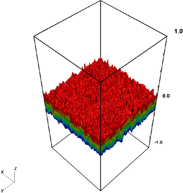
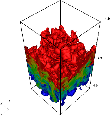
Figure 11: Isosurfaces of temperature at $T=95$ and $T=38$ for the high resolution RTI-unstable simulation with an initially horizontal magnetic field and with $\omega_{c}/\omega_{\mathrm{RTI}}=0.09$ (H2HR in Table 2). The upper panel is at time $t/\sqrt{L/Ag}\approx 1.8$, and the lower panel is at time $t/\sqrt{L/Ag}\approx 4.2$. Temperature contours are also shown on the faces of the simulation domain. At early times, conduction is more important than the RTI, and the temperature contours on the faces of the simulation domain shown in the upper panel show that the temperature mixing layer has diffused substantially. The perturbation on the $T=38$ surface are partly due to the tops of the RTI bubbles which are growing despite the diffusion. These bubbles soon emerge from the diffusion region, as seen in the lower panel.

There is significant growth in magnetic energy for the RTI-unstable simulations (see Fig. 8). Just as the magnetic energy grows exponentially in the RTI-unstable simulation without any explicit conductivity (solid line), the magnetic energy also grows exponentially in the RTI-unstable simulation with an initially horizontal magnetic field (dashed line). The growth rates are similar for both cases, although the growth in the simulation with anisotropic conduction is somewhat slower (i.e., the exponential growth starts later). This is likely because bubbles rise more slowly in the simulations with anisotropic conductivity. By the end of both simulations, the magnetic energy has amplified by about $10^{3}$.

5.2 Vertical magnetic field

We will now describe simulations initialized with a vertical magnetic field. Simulations with $\rho_{+}<\rho_{-}$ are still RTI-stable, but are now HBI-unstable, yielding new dynamics. The simulations with $\rho_{+}>\rho_{-}$ are HBI-stable and RTI-unstable and are similar to the RTI-unstable simulations with horizontal fields. These simulations are not initially in equilibrium, as there is a vertical temperature discontinuity and vertical heat conduction. Physically, the simulations should be viewed as probing length scales much longer than the initial width of the spread in temperature. On these long length scales, the temperature is initially very close to discontinuous.

5.2.1 RTI-stable, HBI-unstable ($\rho_{+}<\rho_{-}$)

We will first investigate the RTI-stable, HBI-unstable case. These runs simulate the discontinuous limit of the HBI. The presence of the HBI in our simulations can be inferred from the height of the temperature mixing layer as a function of time, as shown in Fig. 12. The solid (dashed) lines correspond to simulations with anisotropic (isotropic) conductivity. The dotted line shows the results of our high resolution simulation (VS3HR in Table 2). We find that $h_{T}$ increases as $\sqrt{\chi t}$ for the simulations with isotropic conductivity. For the relatively high conductivity of $\omega_{c}/\omega_{\mathrm{RTI}}=0.09$, the height of the temperature mixing layer is the same for the simulation with anisotropic conductivity (VS2) as for the simulation with isotropic conductivity (VS2I). This is because the HBI has not had enough time to modify the conduction across the entire simulation domain before the temperature mixing layer hits the upper boundary. However, for simulations with $\omega_{c}/\omega_{\mathrm{RTI}}=0.009$ or $0.0009$ the HBI is able to partially inhibit conduction, slowing the growth of the height of the temperature mixing layer.

Figure 12: The height of the temperature mixing layer (defined in §5) as a function of time for our RTI-stable simulations with vertical initial magnetic fields. The solid lines show the results for simulations with anisotropic conductivity, whereas dashed lines show the results for simulations with isotropic conductivity. The top pair of lines, which are overlapping, are for $\omega_{c}/\omega_{\mathrm{RTI}}=0.09$ (VS2 and VS2I in Table 2). The middle set of three lines all correspond to $\omega_{c}/\omega_{\mathrm{RTI}}=0.009$. The solid line has anisotropic conductivity (VS3), the dashed line has isotropic conductivity (VS3I), and the dotted line has anisotropic conductivity, but is at higher resolution (VS3HR). The bottom two lines are for $\omega_{c}/\omega_{\mathrm{RTI}}=0.0009$. For the simulations with relatively small anisotropic conductivities, the HBI becomes non-linear before the temperature mixing layer reaches the upper boundary of the simulation. This results in deviations between the heights from the simulations with isotropic and anisotropic conductivity. The HBI is more effective at diminishing conduction in the high resolution simulation.

The HBI saturates by reorienting vertical field lines to a more horizontal geometry (Parrish & Quataert, 2008). Horizontal fields are produced by strong horizontal flows (McCourt et al., 2011). This reduces the amount of vertical heat conduction, slowing the growth of the temperature mixing layer. In the rapid conduction limit ($\omega_{c}\raisebox{-2.58334pt}{$\,\stackrel{{\scriptstyle\raisebox{-0.60275pt}{$\textstyle>$}}}{{\sim}}\,$}\omega_{\mathrm{buoy}}$), the saturation time-scale is several times the buoyancy time-scale, $\omega_{\mathrm{buoy}}=\sqrt{gd\log T/dz}$. Conversely, if conduction is slow ($\omega_{c}<\omega_{\mathrm{buoy}}$), the saturation time-scale is several times the conduction time-scale. The buoyancy frequency in our simulations is initially very high because of the temperature discontinuity, so the HBI initially grows on the conduction time-scale. Thus, the HBI initially grows more slowly in runs with lower conductivity than in runs with higher conductivity. This is why the HBI has had a more prominent effect on the height in the simulations with $\omega_{c}/\omega_{\mathrm{RTI}}=0.009$ than in the simulations with $\omega_{c}/\omega_{\mathrm{RTI}}=0.0009$ (see Fig. 12). We find that our high resolution simulation exhibits the slowest increase in height of all the HBI-unstable simulations. Due to increased resolution, the field is able to become more horizontal than in the simulations with our fiducial resolution, thereby decreasing the effective vertical conductivity.

Previous simulations of the HBI show that although the field lines never become horizontal, the angle they form with the horizontal decreases as $\sim(t/t_{\mathrm{buoy}})^{-0.85}$ (McCourt et al., 2011), where $t_{\mathrm{buoy}}\sim\omega_{\mathrm{buoy}}^{-1}$. To measure the average orientation of the magnetic field relative to the horizontal, we define $\langle\hat{b}_{z}^{2}\rangle$ to be

$$\left<\hat{b}_{z}^{2}\right>=\left<\frac{B_{z}^{2}}{\boldsymbol{B}\boldsymbol{\cdot}\boldsymbol{B}}\right>,$$ (30)

where $\langle\cdot\rangle$ denotes horizontal average, as above. For simulations with initially vertical magnetic fields, $\langle\hat{b}_{z}^{2}\rangle$ is initially equal to one everywhere.

Figure 13: $\langle\hat{b}_{z}^{2}\rangle$ as a function of height at various times for our high resolution simulation with $\omega_{c}/\omega_{\mathrm{RTI}}=0.009$ (VS3 in Table 2). We plot $\langle\hat{b}_{z}^{2}\rangle$ at $t/\sqrt{L/Ag}=28.2$ (solid line), $56.6$ (dashed line), and $84.8$ (dot-dashed line). The horizontal dotted line shows $\langle\hat{b}_{z}^{2}\rangle=1/3$, which corresponds to an isotropic magnetic field. Due to the action of the HBI, the magnetic field becomes increasingly horizontal as the simulation progresses in time, especially near the centre of the domain where the buoyancy time is the shortest.

In Fig. 13 we plot $\langle\hat{b}_{z}^{2}\rangle$ as a function of height for our high resolution simulation with $\omega_{c}/\omega_{\mathrm{RTI}}=0.009$ (VS3HR in Table 2). If thermal conduction is isotropic, $\langle\hat{b}_{z}^{2}\rangle$ remains close to one for the entire simulation. Figure 13 shows, however, that $\langle\hat{b}_{z}^{2}\rangle$ decreases due to the HBI. We know that the decrease in $\langle\hat{b}_{z}^{2}\rangle$ is not due to random mixing, as $\langle\hat{b}_{z}^{2}\rangle$ decreases to below the isotropic value of $1/3$. There is also an asymmetry between $\langle\hat{b}_{z}^{2}\rangle$ for $z<0$ and for $z>0$. Because the pressure force pushes the interface upwards (see §5.1.1), the HBI acts somewhat more strongly for $z>0$ than for $z<0$, causing $\langle\hat{b}_{z}^{2}\rangle$ to be smaller for $z>0$ than for $z<0$.

We can estimate how the change in orientation of the magnetic field affects the evolution of $h_{T}$. In the HBI non-linear evolution, the magnetic field orientation changes as

$$\langle\hat{b}_{z}^{2}\rangle\sim(t/t_{buoy})^{-1.7}.$$ (31)

As seen in Fig. 13, $\langle\hat{b}_{z}^{2}\rangle$ is a strong function of height. However, for simplicity we will only consider $\langle\hat{b}_{z}^{2}\rangle$ at $z=0$ and only consider heat conduction through the $z=0$ plane. The energy equation implies $dh_{T}/dt\sim\chi_{\mathrm{eff}}/h_{T}$, where $\chi_{\mathrm{eff}}=\chi\langle\hat{b}_{z}^{2}\rangle$. We assume $d\log T/dz\sim 1/h_{T}$ and thus equate $t_{buoy}\sim\sqrt{h_{T}/g}$. One can then show

$$\frac{dh_{T}}{dt}\sim\frac{\chi}{g^{.85}}\frac{1}{h_{T}^{.15}t^{1.7}}.$$ (32)

This implies that $h_{T}$ should converge to a finite value at long times, specifically

$$h_{T}\sim\frac{\chi^{2/3}}{g^{1/3}}.$$ (33)

In this calculation we have neglected terms of order unity. It is unclear if $h_{T}$ is actually converging to a finite value in our simulations that show clear evidence for the HBI. This is not surprising as even our simulations that start with horizontal magnetic fields conduct heat vertically (see §5.1.1). Put another way, finite resolution prevents $\langle\hat{b}_{z}^{2}\rangle$ from decreasing below some minimum value.

In our RTI-stable but HBI-unstable simulations with initially vertical magnetic fields, we find that the evolution of the heights associated with our passive scalars, $h_{C_{L}}$ and $h_{C_{U}}$, are qualitatively similar to the results from the RTI-stable simulations with horizontal initial magnetic fields. Furthermore, the heights are very similar when comparing simulations with isotropic and anisotropic conduction. This is expected at early times, as there is little mixing occurring at the interface until the HBI becomes non-linear. Even in the non-linear phase it is not that surprising that the HBI does not contribute significantly to mixing at the interface: as described in McCourt et al. (2011), the HBI does not excite large velocities during its saturation.

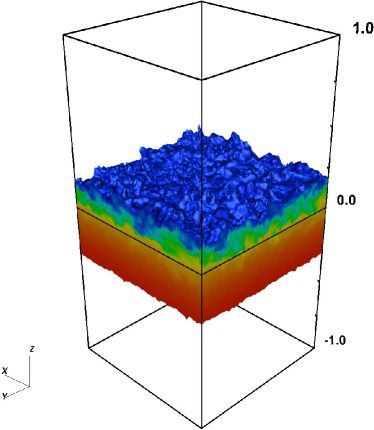
Figure 14: Isosurfaces of fixed composition $C_{U}$ at $C_{U}=0.95$ and $C_{U}=0.05$ for the high resolution RTI-stable, HBI-unstable simulation with $\omega_{c}/\omega_{\mathrm{RTI}}=0.009$ (VS3HR in Table 2) at time $t/\sqrt{L/Ag}=71$. Contours of $C_{U}$ are also shown on the faces of the simulation domain. For simulations with isotropic viscosity $C_{U}$ has very little horizontal variation. Thus, any horizontal structure is due to the HBI.

In Fig. 14 we plot isosurfaces of $C_{U}$ for the high resolution HBI-unstable simulation with $\omega_{c}/\omega_{\mathrm{RTI}}=0.009$ (VS3HR in Table 2). The vertical extent of the composition mixing layer is much smaller than the height of the temperature mixing layer, which is about $0.6$ (see Fig. 12). There are also structures moving horizontally due to the flow produced by the HBI. This motion produces the horizontal magnetic fields which are the saturated state of the HBI.

We can see the magnetic field growth associated with the HBI in Fig. 8. Our high resolution RTI-stable simulation with a vertical initial magnetic field (triple-dot-dashed line) experiences linear growth in magnetic energy starting at $t/\sqrt{L/Ag}\approx 7$. By the end of the simulation the magnetic energy has increased by a factor of nine. The simulation with an initially vertical magnetic field but isotropic conduction exhibits essentially no magnetic field growth. Thus, this linear magnetic field growth is due to the HBI. Because the HBI does not generate large velocities, the growth is not as extreme as in the RTI-unstable simulations.

5.2.2 RTI-unstable, HBI-stable ($\rho_{+}>\rho_{-}$)

The RTI-unstable case with a vertical magnetic field is very similar to the RTI-unstable case with an initially horizontal magnetic field (§5.1.2). We plot the height of the temperature mixing layer as a function of time in Fig. 15. The results are very similar to the corresponding plot in the RTI-unstable case with an initially horizontal magnetic field (Fig. 9). The results are similar because initially both sets of simulations are dominated by vertical heat conduction, but then transition to the RTI at later times. The most prominent difference is that in the initially vertical magnetic field case, when the RTI becomes important the height becomes very close to the height in the fiducial simulation. This is because vertical heat conduction does not impede the rise of RTI bubbles as much as horizontal heat conduction, so diffusive effects slow the rise of RTI bubbles less in the simulations with initially vertical magnetic fields. The RTI bubbles in simulations with initially vertical fields are thinner than the RTI bubbles in simulations with initially horizontal fields, as in our simulation without explicit conductivity (see Fig. 5). As in the RTI-unstable simulations with an initially horizontal magnetic field, the height in the high resolution simulation grows slightly more slowly than at the fiducial resolution.

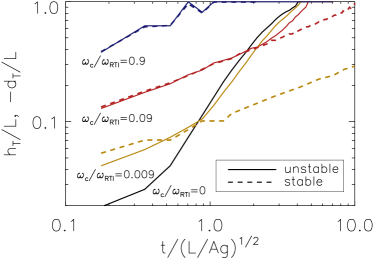
Figure 15: Heights and depths of the temperature mixing layer (defined in §5) as a function of time for simulations with initially vertical magnetic fields, and with various $\omega_{c}/\omega_{\mathrm{RTI}}$. The solid lines show $h_{T}$ for our simulations which are RTI-unstable, whereas the dotted lines show $-d_{T}$ for our simulations which are RTI-stable, and which have isotropic conductivity. The top pair of lines (in blue), which are overlapping, are for $\omega_{c}/\omega_{\mathrm{RTI}}=0.9$ (V1 and VS1I in Table 2). The next pair of lines (in red) are for $\omega_{c}/\omega_{\mathrm{RTI}}=0.09$ (V2 and VS2I). The last set of two lines (in yellow) correspond to $\omega_{c}/\omega_{\mathrm{RTI}}=0.009$ (V3 and VS3I). The bottom solid line shows $h_{T}$ for our fiducial simulation without explicit conductivity (RT in Table 1). The heights for the RTI-unstable runs are about equal to the depths for the RTI-stable runs when conduction dominates over the RTI. When the RTI becomes important, the heights in the RTI-unstable simulations increase in the same way as the height in the fiducial simulation.

The magnetic field growth for the RTI-unstable case with initially vertical field is also similar to the case with initially horizontal field (see Fig. 8). As for all the RTI-unstable simulations, the magnetic energy increases exponentially, and with about the same growth rate as for the simulations with initially horizontal magnetic fields. However, the exponential growth of magnetic energy begins much later (at $t/\sqrt{L/Ag}\approx 3$ rather than $t\approx 0$) in the simulation with an initially vertical magnetic field, and the magnetic energy only amplifies by about $10^{2}$. This is because there is not as much horizontal motion to bend and amplify the initially vertical field lines.

5.3 Skewed magnetic fields

We have also run a set of simulations with initial magnetic fields which make a 45 degree angle with the horizontal (runs A3 and AS2 in Table 2). These were compared to simulations with initially vertical magnetic fields, but with anisotropic thermal conduction with a magnitude one half as large (so the initial vertical heat conduction, proportional to $\chi\langle\hat{b}_{z}^{2}\rangle$, was kept constant). The RTI-stable simulation with an initially skewed magnetic field (AS2) was run with a conductivity of $\omega_{c}/\omega_{\mathrm{RTI}}=0.18$, and is very similar to the RTI-stable simulation with an initially vertical magnetic field, but with $\omega_{c}/\omega_{\mathrm{RTI}}=0.09$ (VS2). We did not run the simulation with a sufficiently low conductivity to see the effects of the HBI, which are presumably not as strong for the simulation with initially skewed magnetic fields.

For RTI-unstable simulations, the simulation with an initially skewed magnetic field and $\omega_{c}/\omega_{\mathrm{RTI}}=0.018$ (A3), and the simulation with an initially vertical magnetic field and $\omega_{c}/\omega_{\mathrm{RTI}}=0.009$ (V3) have the same height initially, when the temperature mixing layer is primarily expanding due to diffusion. However, when the RTI becomes dominant, the height for the simulation with an initially skewed magnetic field is somewhat lower than the height for the simulation with the initially vertical magnetic field. This is because in the RTI-dominated regime, the magnitude of the diffusivity matters more than the direction of the initial field, as the magnetic field becomes isotropized. The simulation with an initially skewed magnetic field has $\omega_{c}/\omega_{\mathrm{RTI}}$ twice as large as the simulation with an initially vertical magnetic field, so this simulation is more dissipative. This causes a slower increase in height.

In physical systems, the magnetic field will never be perfectly aligned or perpendicular to the contact discontinuity. However, these results show that if the magnetic field makes a moderate angle with the contact discontinuity, the behavior is very similar to a system with a vertical magnetic field (see §5.2), but with a smaller conductivity. If the magnetic field makes a small angle with the contact discontinuity, then the evolution will likely be as described by the horizontal magnetic field simulations (see §5.1), which did have some vertical temperature diffusion.

5.4 Additional physical effects

Thermal conduction is anisotropic when the electron gyroradius is much smaller than the electron mean free path. When this is true, the ion gyroradius is often also smaller than the ion mean free path. In this case, viscosity also acts predominantly along magnetic field lines. Because momentum is carried by the ions, the viscosity is smaller than the thermal diffusivity by a factor of about 50 or 100 if $\mu=0.5$ or $1$, respectively. We carried out simulations implementing anisotropic viscosity (as described in Parrish et al., 2012) for contact discontinuities where are RTI-unstable. We found that the height of the temperature mixing layer is not significantly affected by inclusion of anisotropic viscosity. This is probably because the viscosity is so much smaller than the thermal diffusivity. For simulations with an initially horizontal magnetic field, the RTI bubbles were more elongated in the direction of the initial magnetic field than in the simulations with only anisotropic conductivity and numerical viscosity (see also Dong & Stone, 2009).

6 Summary and Discussion

In a dilute magnetized plasma, thermal conduction is anisotropic; this can lead to qualitative changes in the behavior of the plasma. We have investigated the evolution of RTI-stable and RTI-unstable contact discontinuities with anisotropic thermal conduction. The linear problem is only well-posed for a horizontal initial magnetic field. In this case, there is no change to the RTI dispersion relation in the local, Boussinesq limit. In this limit, the classical RTI perturbations are isothermal so they are unaffected by anisotropic conduction (eqn. 18). More generally, compressible perturbations are affected by anisotropic conduction (eqn. 22). If the conduction time-scale is short compared to the growth time of the RTI, perturbations are isothermal and grow faster than the adiabatic perturbations of the classical RTI. The enhancement in the growth rate is modest, but is a function of the temperature contrast across the contact discontinuity and the compressibility of the mode (see Fig. 2).

We have run a number of fully non-linear simulations of contact discontinuities that are either RTI-stable or RTI-unstable, and with several initial magnetic field geometries (see Fig. 1). We focus on initially horizontal and initially vertical magnetic fields – these two choices of the magnetic field orientation bracket the range of dynamics associated with contact discontinuities in dilute plasmas. We primarily used the heights of the temperature and composition mixing layers as diagnostics for the evolution of the initial temperature and density discontinuity. Interestingly, in our high resolution simulation with no explicit conduction (i.e., simulating the classic RTI) the height increases linearly with time in the non-linear phase, rather than quadratically (see Fig. 3). This result is independent of the exact definition of height we use, or when we assume self-similar non-linear growth begins.

In a dilute plasma, the non-linear evolution of a contact discontinuity can be described as a combination of three processes: vertical temperature diffusion, the RTI, and the HBI. For the simulations of RTI-stable contact discontinuities with anisotropic conduction, vertical temperature diffusion is most important. This is true even in our simulations with horizontal initial magnetic fields. The diffusion in this case occurs because we initially perturb the vertical velocity, and subsequent numerical mixing across the interface. Thus, both in simulations with vertical initial magnetic fields and horizontal initial magnetic fields, the height of the temperature mixing layer increases due to diffusion. Although there is significant temperature diffusion, there is not much mixing at the interface in the absence of the RTI, so the height of the composition mixing layer remains small (see Fig. 7).

An RTI-stable contact discontinuity is unstable to the HBI in the presence of vertical magnetic fields; the rate of vertical temperature diffusion across the contact discontinuity slows significantly due to the instability (see Fig. 12). The HBI reorients the vertical magnetic fields to a more horizontal geometry, impeding further heat conduction. We estimate that the HBI would cause a contact discontinuity to spread to a finite width $\sim\chi^{2/3}/g^{1/3}$.

Our simulations with RTI-unstable contact discontinuities initially evolve in the same way as the simulations with RTI-stable contact discontinuities – at early times, the simulations are dominated by temperature diffusion (see, e.g., Fig. 9). However, RTI bubbles are forming and beginning to rise even as the temperature discontinuity diffuses away. The RTI bubbles rise faster and overtake the temperature diffusion, leading to dynamics dominated by the RTI at late times. At this stage, anisotropic conductivity does not play an especially important role. The heights of the RTI bubbles are similar in the simulations with and without anisotropic conductivity. However, the RTI bubbles are a little lower in the simulations with anisotropic conductivity, due to increased dissipation in the system. This is especially true for the simulations with initially horizontal magnetic fields. In this case, the RTI bubbles leak heat to their sides, becoming less buoyant.

We now discuss astrophysical contexts in which our results may be applicable, specifically, supernova remnants, emerging magnetic flux in the solar corona, and cold fronts in galaxy clusters.

Tilley & Balsara (2006) discuss the effects of anisotropic conduction in a supernova remnant. They simulated an entire supernova remnant, but unlike Chevalier et al. (1992) did not find any RTI. Surprisingly, it does not seem that there is significant temperature conduction across their contact discontinuity, as the remnant maintains its spherical shape, instead of becoming more cylindrical as one would expect with their initial magnetic field.

In supernova remnants, the contact discontinuity feels an effective gravitational force due to its deceleration into the ambient medium. The magnitude of the acceleration is decreasing with time as $g_{\mathrm{eff}}\sim t^{-8/5}$ (e.g., Sedov, 1946). Thus, one might expect the height of RTI bubbles to increase as $g_{\mathrm{eff}}t^{2}\sim t^{2/5}$. At late times this is slower than the diffusive growth of the height of the temperature mixing layer, which grows as $\sqrt{\chi t}$. As an example, assume a supernova remnant with an electron temperature of $T=10^{8}\;\mathrm{K}$ and number density $n=4\;\mathrm{cm}^{-3}$ is expanding into a medium with $n=1\;\mathrm{cm}^{3}$. Then we have that the height of the temperature mixing layer due to temperature diffusion after a Sedov time $\sim 100\;\mathrm{yr}$ is

$$\sqrt{\chi t}\sim 3\;\mathrm{pc}\;\left(\frac{t}{100\;\mathrm{yr}}\right)^{1/2}.$$ (34)

After $\sim 100\;\mathrm{yr}$ the remnant would expand to a radius of about $r\sim 2\;\mathrm{pc}$, so $g_{\mathrm{eff}}\sim r/t^{2}\sim 0.6\;\mathrm{cm}\;\mathrm{s}^{-2}$. We find that the height of the highest RTI bubble after $100\;\mathrm{yr}$ would be about

$$g_{\mathrm{eff}}t^{2}\sim 2\;\mathrm{pc}\;\left(\frac{t}{100\;\mathrm{yr}}\right)^{2/5}.$$ (35)

This suggests that diffusion and RTI dynamics are about equally important after a Sedov time, although diffusion would likely dominate at later times. Thus, a global simulation of an entire supernova remnant would be necessary to accurately determine how anisotropic conduction affects the contact discontinuity.

Berger et al. (2011) recently reported observations of hot, dilute solar prominences. They interpret the observations as showing the RTI on the surface of the bubble of hot plasma, as described in numerical simulations (e.g., Isobe et al., 2005). They report temperatures of the hot plasma to be $T\approx 10^{6}\;\textrm{K}$, which, using $n\approx 10^{9}\;\textrm{cm}^{-3}$, gives a collision frequency of $\nu\approx 10^{2}\;\textrm{Hz}$. This is much smaller than the electron gyrofrequency $\omega_{\mathrm{ce}}\approx 10^{7}(B/1\;\mathrm{G})\;\mathrm{Hz}$, indicating the heat conduction is primarily along magnetic field lines. Furthermore, such a plasma would have a parallel heat diffusivity of $\approx 10^{16}\;\mathrm{cm}^{2}\;\mathrm{s}^{-1}$ (Spitzer, 1962), so the diffusion time across a prominence which has a size $\approx 10^{9}\;\mathrm{cm}$ is about $100\;\mathrm{s}$. This is much shorter than the evolution time for the prominence, which is on order an hour. Since conduction becomes increasingly important at smaller length scales, this shows that anisotropic conduction should be important for the RTI discussed in Berger et al. (2011).

The magnetic field in prominences is believed to be parallel to the interface of the prominence. If some field lines were perpendicular to the interface, then heat conduction would quickly smear out the interface (see §5.2.2). However, the observations show that the prominences hold their shape on time-scales of an hour. Thus, we can take the magnetic fields to be primarily along the interface. Our linear results in §2 show that the growth of the RTI should be faster than would be predicted without anisotropic conduction, though how much faster depends on the compressibility of the modes. In the non-linear regime (§5.1.2), we expect a superposition of spreading of the interface due to perpendicular heat diffusion and a somewhat slower RTI growth. Because perpendicular diffusion is not very important (the perpendicular diffusivity is smaller by a factor of $(\nu/\omega_{\mathrm{ce}})^{2}$), we expect the non-linear behavior to be similar to the RTI without conduction.

Our calculations are not ideally suited for comparison with solar prominences as we have assumed that the magnetic fields are dynamically unimportant, which is not the case for solar prominences. Strong magnetic fields inhibit motions which bend the field lines, instead favoring interchange-like motions (SG07). Anisotropic viscosity along field lines also would inhibit motion along field lines (Dong & Stone, 2009).

Parrish & Quataert (2008) and Birnboim et al. (2010) suggested that thermal diffusion across the contact discontinuities found at cold fronts in galaxy clusters could be suppressed by the HBI. In §5.2.1 we determined that the HBI will cause the contact discontinuity to diffuse to a finite width $\sim\chi^{2/3}/g^{1/3}$. Birnboim et al. (2010) simulate shocks propagating through a galaxy cluster which merge producing a cold front. Using their cluster parameters for a front at $200\;\mathrm{kpc}$, we find that $\chi\approx 3\times 10^{30}\;\mathrm{cm}^{2}\;\mathrm{s}^{-1}$, and $g\approx 10^{-8}\;\mathrm{cm}\;\mathrm{s}^{-2}$. This gives the saturation width of the contact discontinuity to be $\sim 30\;\mathrm{kpc}$, which is somewhat larger than the Chandra upper limit of $10\;\mathrm{kpc}$. The saturation width of the cold front observed in the galaxy cluster A3667 (Vikhlinin et al., 2001) can be estimated to also be $\sim 40\;\mathrm{kpc}$ – much larger than the observed width $\leq 5\;\mathrm{kpc}$. Furthermore, our numerical results in §5.2.1 suggests that the saturation width is likely a few times $\chi^{2/3}/g^{1/3}$. These results suggest that additional effects not included in our simple model might be required to explain the narrow widths of observed cold fronts.

Appendix A Calibration of Linear Growth Rates using Numerical Simulations

We have tried to confirm the growth rates derived in §2 through numerical simulations. Our numerical methodology is summarized in §3. There are two difficulties that make accurate comparison between linear theory and the numerical results impossible. The first difficulty is that the fastest growing modes are those on the smallest length scale allowed in the simulation. The second difficulty is that viscous effects will act to slow the growth of the instability. Although we do not implement an explicit viscosity in our numerical simulations (see §3), there is numerical diffusion which adds an effective viscosity to the problem. This viscosity will damp out any modes with wavelengths smaller than a cutoff wavelength, which is the width of a few grid points – we will refer to this cutoff wavelength as the viscous length scale. The fastest growing modes will be those with a wavelength only slightly larger than this viscous length scale. Thus, these modes are substantially affected by viscosity, and cannot be accurately compared to our calculations above which are for the inviscid RTI problem.

A possible way to get around these difficulties would be to only excite long wavelength modes which are not affected by viscosity. However, rounding errors produce random perturbations at the smallest scales in the simulation, and these random perturbations grow faster than the long wavelength modes of interest (as their growth rates are many times larger than the growth rates of the modes of interest). If we increase the amplitude of the initial perturbations, it will take longer for the random noise to grow to the same size as the initial perturbation. Unfortunately, non-linear effects become important at these higher amplitudes, so we still cannot accurately measure the linear growth rate.

We have tried using the eigenfunctions from the calculation in §2 as an initial perturbation, in hopes of seeing some growth due to the initial perturbation before the simulation is overwhelmed by the small scale modes. Unfortunately, the cusp in the perturbation vertical velocity and discontinuities in perturbation horizontal velocity, density, and pressure at $z=0$ are not resolved by the simulation. Because of this, using the eigenfunctions as an initial perturbation launches sound waves with amplitudes similar to the amplitude of the initial perturbation. These obfuscate the growth of the mode of interest. To summarize, we have sound waves launched by the initial perturbation which dominate the dynamics at the beginning of the simulation, and quickly growing small scale modes which dominate later on in the simulation. Between these two effects, we are unable to measure the growth of the longer wavelength modes which are relatively unaffected by viscosity. Presumably these difficulties could be remedied by using a resolved density profile rather than a true discontinuity on the grid scale. However, we concluded that there was not sufficient motivation to do so given that our numerical methods have been validated using many other tests (in particular, see Parrish & Stone (2005) and Sharma & Hammett (2007) for tests of the anisotropic conduction methods).

References

- Balbus (2000) Balbus S. A., 2000, ApJ, 534, 420
- Balsara et al. (2008a) Balsara D. S., Bendinelli A. J., Tilley D. A., Massari A. R., Howk J. C., 2008a, MNRAS, 386, 642
- Balsara et al. (2008b) Balsara D. S., Tilley D. A., Howk J. C., 2008b, MNRAS, 386, 627
- Berger et al. (2011) Berger T. et al., 2011, Nature, 472, 197
- Birnboim et al. (2010) Birnboim Y., Keshet U., Hernquist L., 2010, MNRAS, 408, 199
- Braginskii (1965) Braginskii S. I., 1965, Reviews of Plasma Physics, 1, 205
- Chandrasekhar (1961) Chandrasekhar S., 1961, Hydrodynamic and hydromagnetic stability, Chandrasekhar, S., ed.
- Chevalier et al. (1992) Chevalier R. A., Blondin J. M., Emmering R. T., 1992, ApJ, 392, 118
- Cunningham et al. (2011) Cunningham A. J., Klein R. I., Krumholz M. R., McKee C. F., 2011, ApJ, 740, 107
- Dimonte et al. (2004) Dimonte G. et al., 2004, Physics of Fluids, 16, 1668
- Dong & Stone (2009) Dong R., Stone J. M., 2009, ApJ, 704, 1309
- Gardiner & Stone (2008) Gardiner T. A., Stone J. M., 2008, Journal of Computational Physics, 227, 4123
- Gull (1973) Gull S. F., 1973, MNRAS, 161, 47
- Isobe et al. (2005) Isobe H., Miyagoshi T., Shibata K., Yokoyama T., 2005, Nature, 434, 478
- Jun & Norman (1996) Jun B.-I., Norman M. L., 1996, ApJ, 465, 800
- McCourt et al. (2011) McCourt M., Parrish I. J., Sharma P., Quataert E., 2011, MNRAS, 413, 1295
- Parrish et al. (2012) Parrish I. J., McCourt M., Quataert E., Sharma P., 2012, ArXiv e-prints
- Parrish & Quataert (2008) Parrish I. J., Quataert E., 2008, ApJL, 677, L9
- Parrish & Stone (2005) Parrish I. J., Stone J. M., 2005, ApJ, 633, 334
- Parrish & Stone (2007) Parrish I. J., Stone J. M., 2007, ApJ, 664, 135
- Quataert (2008) Quataert E., 2008, ApJ, 673, 758
- Robinson et al. (2004) Robinson K. et al., 2004, ApJ, 601, 621
- Sedov (1946) Sedov L. I., 1946, Journal of Applied Mathematics and Mechanics, 10, 241
- Sharma & Hammett (2007) Sharma P., Hammett G. W., 2007, Journal of Computational Physics, 227, 123
- Shivamoggi (2008) Shivamoggi B. K., 2008, ArXiv e-prints
- Spitzer (1962) Spitzer L., 1962, Physics of Fully Ionized Gases, Spitzer, L., ed.
- Stone & Gardiner (2007) Stone J. M., Gardiner T., 2007, Physics of Fluids, 19, 094104
- Stone et al. (2008) Stone J. M., Gardiner T. A., Teuben P., Hawley J. F., Simon J. B., 2008, ApJS, 178, 137
- Tilley & Balsara (2006) Tilley D. A., Balsara D. S., 2006, ApJL, 645, L49
- Vikhlinin et al. (2001) Vikhlinin A., Markevitch M., Murray S. S., 2001, ApJ, 551, 160