Magnetic properties and critical behavior of disordered Fe_1-xRu_x alloys: a Monte Carlo approach

Abstract

We study the critical behavior of a quenched random-exchange Ising model with competing interactions on a bcc lattice. This model was introduced in the study of the magnetic behavior of Fe_1-xRu_x alloys for ruthenium concentrations $x=0\%$, $x=4\%$, $x=6\%$, and $x=8\%$. Our study is carried out within a Monte Carlo approach, with the aid of a re-weighting multiple histogram technique. By means of a finite-size scaling analysis of several thermodynamic quantities, taking into account up to the leading irrelevant scaling field term, we find estimates of the critical exponents $\alpha$, $\beta$, $\gamma$, and $\nu$, and of the critical temperatures of the model. Our results for $x=0\%$ are in excellent agreement with those for the three-dimensional pure Ising model in the literature. We also show that our critical exponent estimates for the disordered cases are consistent with those reported for the transition line between paramagnetic and ferromagnetic phases of both randomly dilute and $\pm J$ Ising models. We compare the behavior of the magnetization as a function of temperature with that obtained by Paduani and Branco (2008), qualitatively confirming the mean-field result. However, the comparison of the critical temperatures obtained in this work with experimental measurements suggest that the model (initially obtained in a mean-field approach) needs to be modified.

I Introduction

We study the magnetic properties and critical behavior of a quenched random-exchange Ising model, through extensive Monte Carlo simulations. Our starting point was the model proposed in Ref. nilton:feru, , consisting of iron and ruthenium atoms randomly distributed in a body-centered cubic (bcc) lattice, with probabilities $1-x$ and $x$, respectively. In this model, atoms are treated as Ising spins, Fe-Fe bonds are ferromagnetic (FM), with exchange integral $J$, while Fe-Ru and Ru-Ru interactions are antiferromagnetic (AF) with exchange integrals $-\lambda J$ and $-\xi J$, respectively, where $\lambda$ and $\xi$ depend on the ruthenium concentration, $x$, as follows: $\lambda\equiv\xi=\xi_{0}-\xi_{1}x$. The parameters $\xi_{0}$ and $\xi_{1}$ were determined from the experimental values for the critical temperatures of the system for some concentrations of ruthenium, reported in Ref. artigo:paduani, , by fitting these data to the mean-field solution of the model.

The main goal of this work is to establish the universality class of the spin model introduced in Ref. nilton:feru, , through extensive numerical calculations of some of its thermodynamic quantities. We used the metropolis algorithm to generate the data and employed re-weighting techniques and finite-size scaling (FSS) analysis. We also compare the behavior of thermodynamic quantities obtained by Monte Carlo simulations with experimental and mean-field results. We compare the values of $T_{c}(x)$ with the experimental measurements artigo:paduani and theoretical estimates nilton:feru to determine if the model for the Fe_1-xRu_x alloys remains adequate in a non-mean-field approach. In this later work, the parameters of the proposed Hamiltonian were obtained through a fit of the theoretical critical temperatures, obtained in a mean-field-like approximation, with the measured values reported in Ref. artigo:paduani, . The mean-field result is obtained using the Bogoliubov inequality, in a similar fashion as the one employed in the study of order-disorder transitions through a cluster variational method kikuchi1980 .

An important aspect of this work is the FSS analysis to determine the critical exponents. The study of this model is mainly an investigation of the effects of quenched disorder on the critical behavior of a system of Ising spins, like so many theoretical and experimental examples presented throughout the last three decades or more. An interesting fact of these disordered systems is the theoretical prediction that the introduction of disorder must change the universality class of the system if $\alpha>0$, where $\alpha$ is the specific heat critical exponent for the pure system. This result is known as the Harris criterion livro:cardy . The $\alpha>0$ condition is satisfied for the case of the pure Ising model in three dimensions, so we can expect three-dimensional disordered Ising models to belong to another universality class, when compared to their uniform counterparts. However, the Harris criterion says nothing about the new universality class. Renormalization-group arguments infer that the universality class of the disordered three-dimensional Ising model does not depend on the concentration $x$. Moreover, experimental results show that, for small concentrations $x$ of AF impurities (as in Fe_1-xMn_x, Fe_1-xZn_xF₂ and Fe_1-xRu_x alloys) or nonmagnetic impurities (as in Fe_1-xAl_x alloys), these systems have a continuous transition between a ferromagnetic and a paramagnetic phase at a temperature $T_{c}(x)<T_{c}(x=0\%)$, with a critical behavior clearly different from the case without disorder ($x=0\%$), but that seems to be independent of the concentration $x$, within the experimental precision belanger2000 . By small concentrations we mean $x<x_{c}$ for nonmagnetic impurities, where $x_{c}$ is the critical concentration above which there is only a single paramagnetic phase hasenbusch2007uc . In the case of AF impurities, we mean $x<x_{g}$, where $x_{g}$ is the concentration for which the transition line between paramagnetic and ferromagnetic phases meets the transition line between paramagnetic and spin-glass phases, where frustration is relevant livro:barkema .

It is curious that, contrary to experimental results, Monte Carlo simulations presented a wide range of different values for the critical exponents of these disordered systems, all seeming to indicate some sort of dependence between universality class and impurity concentration. Only recently (late 1990’s onward), with the growth of processor capacity and available resources for simulations, is theoretical research heading toward a solution to this apparent inconsistency, and studies have shown that critical exponents are independent of impurity concentration along the transition line between paramagnetic and ferromagnetic phases in disordered Ising models ballesteros1998 ; calabrese2003tdr ; hasenbusch2007uc ; hasenbusch2007+-J . These works have shown the importance of a careful analysis of the scaling behavior of thermodynamic functions, taking into account finite-size correction terms due to irrelevant fields in the Hamiltonian, for a correct assessment of the critical exponents of these systems.

At first glance, one could suspect that our model does not belong to any of the previously discussed universality classes. However, we could think of it as a member of a more general family of models with bonds $+J$ and $-rJ$ randomly distributed with probabilities $1-p$ and $p$ respectively. We obtain the Ising model with randomly diluted bonds (RBIM) as $r=0$, the Ising model with $\pm J$ random bonds for $r=1$ and our model for some combinations of $r$ and $p$. Note also that the Fe_1-xRu_x system we study in this work has a crossover to the Ising Model with randomly diluted sites (RSIM) when $x=10\%$. Therefore, we make the hypothesis that our model belongs to the RSIM-RBIM universality class, as is the case also for the paramagnetic-ferromagnetic transition line of the $\pm J$ Ising model hasenbusch2007uc ; hasenbusch2007+-J . In this sense, our Fe_1-xRu_x system would be somewhere in between the $r=0$ and $r=1$ limits. To assess this possibility, we have performed extensive Monte Carlo simulations, with the important inclusion of correction-to-scaling terms, as discussed in the previous paragraph, in order to estimate the critical exponents and critical temperatures of the model introduced in Ref. nilton:feru, . This model is explained in Sec. II, the simulation and data analysis methods are discussed in Secs. III and IV respectively and our results are presented and discussed in Sec. V.

II Model

Ref. artigo:paduani, shows that Fe_1-xRu_x alloys are found in the bcc structure for $x<30\%$ whereas, for $x\approx 30\%$, the system undergoes a crystallographic transition to an hcp structure. While in the bcc structure, the lattice parameter increases steadily with the Ruthenium concentration $x$ and the system has a ferromagnetic-paramagnetic phase transition at $T_{c}(x)$, as seen in Tab. 1. In Ref. nilton:feru, , the authors present a detailed discussion of experimental results and first-principle electronic-structure calculations that provide evidence that ferromagnetic Fe-Fe bonds and antiferromagnetic Fe-Ru and Ru-Ru bonds should effectively model the Fe_1-xRu_x system.

Table 1: Experimental values of critical temperatures for Fe_1-xRu_x alloys, taken from Ref. artigo:paduani, .

$x$	$T_{c}~{}(K)$
$0\%$	1043
$2\%$	968(2)
$4\%$	928(2)
$6\%$	908(2)
$10\%$	838(2)

The model proposed by Paduani and Branco (2008) consists of Fe and Ru atoms randomly distributed on a bcc lattice with probabilities $1-x$ and $x$ respectively. Each atom has a magnetic degree of freedom that is assumed to behave as an Ising-like spin, so the system is described by a spin-1/2 Ising Hamiltonian

$$\mathcal{H}=-\sum_{\left\langle i,j\right\rangle}J_{ij}\sigma_{i}\sigma_{j},$$ (1)

where the sum goes over all nearest-neighbor pairs, $\sigma_{i}=\pm 1$ for all sites $i$, and the exchange integral $J_{ij}$ takes the values $J$ for Fe-Fe bonds, $-\lambda J$ for Fe-Ru bonds, and $-\xi J$ for Ru-Ru bonds.

A mean-field solution nilton:feru of Hamiltonian (1), using the Bogoliubov inequality livro:callen ; livro:julia , yields

$$\left\{\frac{(1-x)^{2}}{1+\exp(-2J/k_{B}T_{c})}+\frac{2x(1-x)}{1+\exp(2\lambda J/k_{B}T_{c})}+\frac{x^{2}}{1+\exp(2\xi J/k_{B}T_{c})}\right\}=\frac{4}{7}.$$ (2)

In Ref. nilton:feru, , the authors assume that $\lambda=\xi\equiv\xi_{0}-\xi_{1}x$ and present a least-square fit of Eq. (2) to the experimental values of $T_{c}$ in Tab. 1. The values reported for the parameters are $\xi_{0}=0.54(2)$ and $\xi_{1}=5.4(4)$, so that the final form of the Hamiltonian reads:

$$\mathcal{H}=-J\sum_{\left\langle i,j\right\rangle}\zeta_{ij}\sigma_{i}\sigma_{j}$$ (3)

where

$$\zeta_{ij}=\left\{\begin{array}[]{lll}\zeta_{\mbox{\scriptsize{}}}&=&1\\ \zeta_{\mbox{\scriptsize{}}}&=&-(0.54-5.4x)\\ \zeta_{\mbox{\scriptsize{}}}&=&-(0.54-5.4x),\end{array}\right.$$ (4)

and the spin variables $\sigma_{i}$ take the values $\pm 1$ and the sum goes over all nearest-neighbor pairs.

III Monte Carlo Simulations

We studied the three-dimensional Ising system described by the Hamiltonian (3) within a Monte Carlo (MC) approach. We have employed the metropolis algorithm artigo:metropolis ; livro:barkema to simulate bcc lattices with $2L^{3}$ sites, periodic boundary conditions, and several system sizes $L$, ranging from 5 to 50. Each site on the lattice is randomly chosen to be an Fe or Ru atom with probabilities $1-x$ and $x$, respectively. All random numbers were generated using a Tausworthe (shift-register) generator artigo:shift-register with “magic numbers” $p=1279$ and $q=1063$ artigo:landau ; shan-ho:private .

A Monte Carlo step per spin (MCS) corresponds to $N=2L^{3}$ attempts to flip a single spin, chosen at random, or a full sweep on the lattice, when we perform sequential updates. As the sequential algorithm proved to be far more efficient in generating independent states than the more traditional random choice, it was the one used for most of our simulations. The comparison between these two procedures is presented in Subsec. V.2.

Our largest simulations ran up to $4.5\times 10^{7}$ MCSs and we made sure to generate at least $n=8000$ uncorrelated states, with $n$ given by

$$n=\frac{n_{\mbox{\scriptsize{}}}-t_{\mbox{\scriptsize{}}}}{2\tau},$$ (5)

where $n_{\mbox{\scriptsize{}}}$ is the number of MCSs, $t_{\mbox{\scriptsize{}}}$ is the equilibration time and $\tau$ is the largest correlation time estimated by the integral method livro:barkema . As it is the case for the metropolis dynamics, the largest correlation time is, in general, obtained from the magnetization autocorrelation function. Therefore, in our case, $\tau$ refers to the magnetization correlation time.

For practical reasons concerning data storage, we have only saved simulation data every 10 MCS. However, we have rescaled our dynamic calculations and present all correlation times in units of one MCS. This rescaling introduces a systematic error on the integral correlation time when typical values of $\tau$ are close to 10 MCS or smaller, as shown in Sec. V.2. This error is due to the numerical integration using the trapezoid rule, as the integral of an exponential decay approaches the exact value from above with numerical error of the order $\sim\mathcal{O}(n^{-2})$ livro:calculo-numerico , where $n$ is the number of bins. We checked for systematic deviation by comparing pairs of $\tau$ estimates obtained from the same simulation considering a time unit of 1 MCS and 10 MCS. We found no systematic error for $L\geq 15$ and, since $\tau$ is overestimated, it does not affect the precision of our equilibrium analysis.

When performing Monte Carlo simulations it is customary to work with the dimensionless coupling constant $K=J/(k_{B}T)$ and dimensionless temperature $\bar{T}=1/K$. We also define other dimensionless thermodynamic quantities such as the extensive energy

$$E=-\sum_{\left\langle i,j\right\rangle}\zeta_{ij}\sigma_{i}\sigma_{j},$$ (6)

magnetization per spin

$$m=\frac{1}{N}\sum_{i=1}^{N}\sigma_{i},$$ (7)

specific heat

$$c=\frac{K^{2}}{N}\left[\langle E^{2}\rangle-\langle E\rangle^{2}\right],$$ (8)

magnetic susceptibility per spin

$$\chi=\frac{N}{K}\left[\langle m^{2}\rangle-\langle|m|\rangle^{2}\right],$$ (9)

the quadratic cumulants

$$U_{22}=\frac{[\langle m^{2}\rangle^{2}]-[\langle m^{2}\rangle]^{2}}{[\langle m^{2}\rangle]^{2}}$$ (10)

and

$$U_{4}=\frac{[\langle m^{4}\rangle]}{[\langle m^{2}\rangle]^{2}},$$ (11)

and the more traditional Binder’s cumulant

$$U\equiv 1-\frac{1}{3}U_{4}.$$ (12)

On all equations above, $\langle\cdots\rangle$ denotes thermal averages whereas $[\cdots]$ denotes averages over disorder configurations.

For each pair of $x$ and $L$ values, we ran simulations at different temperatures near the critical point (up to 20 temperatures for smaller lattices and 5 for $L>30$) and used the multiple-histogram method artigo:ferrenberg:histograma1 ; artigo:ferrenberg:histograma2 ; livro:barkema to compute quantities of interest over an almost continuous range of temperatures. The thermal error associated with those quantities is estimated by dividing the data from each simulation in blocks and repeating the multiple-histogram process for each block. The errors are the standard deviation of the values obtained for a given quantity on the different blocks. For each set of parameters ($L$, $x$, $T$) we average over $N_{S}$ samples of atomic disorder. We chose $10\leq N_{S}\leq 20$, such that the error due to disorder was of the same magnitude or smaller than the thermal error obtained for each disorder configuration. Finally, we sum both thermal and disorder errors for an estimate of the total error.

IV Data analysis

In MC simulations we necessarily deal with finite systems. However, our interest lies in critical phenomena, which happen in the thermodynamic limit. The critical behavior of such systems may be extracted from finite systems by examining the size dependence of the singular part of the free energy density livro:julia . In this finite-size scaling approach we write the free energy density for a system of linear size $L$ near the critical point as

$$\bar{f}_{\mbox{\scriptsize{}}}(t,h,L)\sim L^{-d}f^{0}(tL^{y_{t}},hL^{y_{h}},\{\bar{u}_{i}L^{-\omega_{i}}\})$$ (13)

where $t$ is the reduced temperature and is given by $(T-T_{c})/T_{c}$, $H$ is the external magnetic field, and $h=H/(k_{B}T)$. We assume that $t$ and $h$ are the only relevant fields while $\bar{u}_{i}$ are irrelevant perturbations, such that $\omega_{i}>0$, which ensures that in the thermodynamic limit, as $\bar{u}_{i}L^{-\omega_{i}}\rightarrow 0$, our free energy is a function only of relevant fields.

Taking appropriate derivatives of the free energy, it is possible to show that some thermodynamic quantities $Q$ (such as magnetization, specific heat, and magnetic susceptibility) may be written in the following scaling form:

$$Q=Q_{0}L^{\theta}\left\{1+\sum_{i}Q_{i}L^{-\omega_{i}}+\cdots\right\},$$ (14)

where $\theta$ is related to the traditional exponents. As (14) will be used to fit numerical data to estimate critical exponents, we have to truncate the sum at some point. As each additional exponent $\omega_{i}$ taken into account will add two free parameters to an eventual fit and that reduces drastically the number of degrees of freedom, we considered only the first exponent $\omega_{1}\equiv\omega$. We then have

$$m =m_{0}L^{-\beta/\nu}\left\{1+m_{1}L^{-\omega}\right\},$$ (15)

$$\chi =\chi_{0}L^{\gamma/\nu}\left\{1+\chi_{1}L^{-\omega}\right\},$$ (16)

$$c =c_{0}L^{\alpha/\nu}\left\{1+c_{1}L^{-\omega}\right\}.$$ (17)

A similar scaling behavior near the critical point holds for the derivatives

$$\frac{dG}{dK}=G_{0}L^{1/\nu}\left\{1+G_{1}L^{-\omega}\right\},$$ (18)

where $G$ stands for the Binder’s cumulant $U$ or quantities linked to the magnetization, such as $\ln{\langle|m|\rangle}$, $\ln{\langle m^{2}\rangle}$, and $\ln{\langle|m|^{n}\rangle}$ artigo:landau . Equation (18) is particularly useful to determine the exponent $\nu$. Finally, for the critical temperature we have

$$T_{c}(L)=T_{c}+A_{0}L^{-1/\nu}\left\{1+A_{1}L^{-\omega}\right\},$$ (19)

where $T_{c}(L)$ is the pseudo-critical temperature for a given system size $L$, and $T_{c}$ is the true critical temperature.

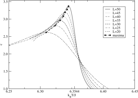
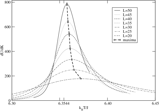
Figure 1: Thermodynamic quantities versus dimensionless temperature $\bar{T}$ for $x=0\%$ and lattice sizes ranging from 20 to 50. In (a) we plot the specific heat and in (b) the slope $dU/dK$ of the Binder’s cumulant. The lines were obtained with the multiple histogram method, the symbols represent the location of the peaks for each lattice size and the dashed line connecting the peaks is a guide to the eye. The tick in $\bar{T}=6.3544$ corresponds to our estimate of the critical temperature. The data in this figure and in all other figures in this work were plotted with their respective error bars; however, some error bars are smaller then the symbols.

We perform least square fits using expressions (15)-(19) with all quantities computed at several temperatures close to $T_{c}$. These estimates of $T_{c}(L)$ are obtained locating the temperatures $T_{m}$ where we find the maxima of several quantities which diverge as $L\rightarrow\infty$ ($c$, $\chi$, $\frac{d\langle m\rangle}{dK}$, $\frac{dU}{dK}$) as well as the temperatures $T_{f}$ at which the cumulants $U_{4}$, $U_{22}$, and $U_{d}\equiv U_{4}-U_{22}$ assume particular fixed values. The fixed values used were MC estimates of the universal values these cumulants assume at the critical point on randomly site-diluted (RSIM) and bond-diluted (RBIM) Ising models: $U_{4}=1.648(3)$, $U_{22}=0.148(1)$ and $U_{d}=1.500(1)$ hasenbusch2007uc . The calculation of the relevant quantities for different temperatures is done using the multiple-histogram method. Examples of this procedure are shown in Fig. 1 for the specific heat and for the derivative of the Binder cumulant, both used to locate different estimates of $T_{m}$. The comparison between the results from both $T_{m}$ and $T_{f}$ FSS methods provides an additional way to check if our model belongs to the RSIM-RBIM universality class.

Equations (15)-(19) all have four free parameters to be adjusted in the fitting process and no stable fits were possible for our data, meaning our statistics should be increased if we desire to obtain the exponents $\alpha$, $\beta$, $\gamma$, $\nu$, and $\omega$ independently. Since we are more interested in obtaining $\alpha$, $\beta$, $\gamma$, and $\nu$ than in finding precise correction-to-scaling exponents $\omega$, we employ a procedure similar to the one presented in Ref. artigo:landau, , in which we set a fixed value for exponent $\omega$ and perform a fit with three free parameters, instead of four. Than we change the fixed value of $\omega$ and keep performing fits to obtain the values of the other exponents. Once several fits are made, we locate the interval of values of $\omega$ such that we minimize the values of the variance of residuals, $\chi^{2}/\mbox{DOF}$, where DOF is the number of degrees of freedom of the fit. We repeat this procedure using system sizes $L_{\mbox{\scriptsize{min}}}\leq L\leq 50$, with $L_{\mbox{\scriptsize{min}}}=$ 5, 10, 12, 15, 18, 20, and 25 to obtain the $L_{\mbox{\scriptsize{min}}}$ that globally minimizes $\chi^{2}/\mbox{DOF}$. Once the best $L_{\mbox{\scriptsize{min}}}$ and corresponding series of values for $\omega$ are located, we average the values obtained for the exponents, making sure to include only fits with $\chi^{2}/\mbox{DOF}<1.0$ in this statistical analysis.

V Results and Discussion

V.1 Simulation strategy and preliminary results

For the pure case ($x=0\%$), we ran simulations at $\bar{T}=\bar{T}_{c}^{\mbox{\scriptsize{}}}=6.35435$, which corresponds to the high-temperature series estimate $K_{c}^{\mbox{\scriptsize{}}}=0.1573725(6)$ of the critical coupling for the pure Ising model on a bcc lattice artigo:butera . We used the single-histogram method artigo:ferrenberg:histograma1 ; livro:barkema to locate the temperatures where the peaks of the thermodynamic quantities of interest occurred. From the peak locations we chose temperatures to perform new simulations. Finally, we employ the multiple-histogram re-weighting using the data from at least five simulations at different temperatures such that all peaks were found within the interval between the minimum and maximum of those temperatures.

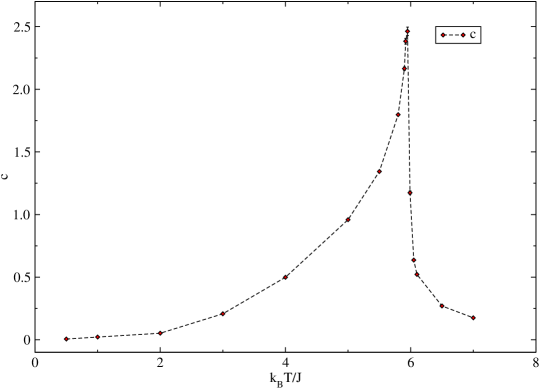
Figure 2: Specific heat versus $\bar{T}$ for $x=6\%$ and $L=30$. The points represent the simulation data and the dashed line is a guide to the eye.

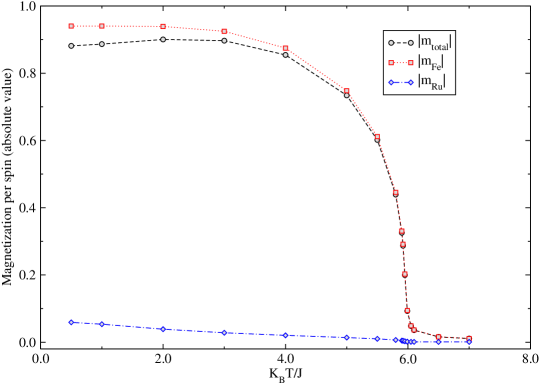
Figure 3: (Color online) Total magnetization per spin and individual contributions of Fe and Ru atoms for the magnetization versus $\bar{T}$, obtained for $x=6\%$ and $L=30$. The points represent the simulation data and the lines are only a guide to the eye.

A similar procedure was employed for the disordered case ($x=4\%$, $6\%$ and $8\%$). However, since no previous estimates for $T_{c}$ were available, we performed test simulations over a wide range of temperatures, in order to make a rough estimate of the location of the critical region. Figures 2 and 3 exemplify this initial attempt to determine $T_{c}(L)$ for $x=6\%$ and $L=30$. Once determined a suitable temperature interval for each concentration $x$ and size $L$, we divided it in five ($L>30$) to eleven (smaller lattices) temperatures, to simulate and employ the multiple-histogram method as discussed above.

One interesting aspect of Fig. 3, besides the additional $T_{c}$ estimate it provides, is the behavior of the magnetization as a function of temperature. We observe a slight decrease in the total magnetization at low temperatures, when we approach $T=0$. This decrease is also present in the mean-field approximation to this model (see Fig. 2 in Ref. nilton:feru, ). Although not as pronounced as the effect presented in Ref. nilton:feru, , it also occurs in our Monte Carlo approach; thus, it is not a mean-field-only effect. For comparison between Fig. 3 and Fig. 2 in Ref. nilton:feru, , it is important to stress that the lowest temperature we simulated is $\bar{T}=0.5$, which corresponds to $T\approx 80~{}K$ (this value is obtained using $J=14.16~{}meV$, as discussed in Sec. V.4).

It is possible to present a qualitative description of this effect. The probability that a Ru atom is completely surrounded by Fe atoms as nearest-neighbors is $(1-x)^{8}$, which is quite high for low Ru concentrations ($\approx 51\%$ for $x=8\%$, $\approx 61\%$ for $x=6\%$, $\approx 72\%$ for $x=4\%$, $\approx 85\%$ for $x=2\%$ etc). Next, let us consider a scenario in which the great majority of Ru atoms have no Ru first neighbors. In a situation like this, there is close to no frustration and for $T=0$ we expect almost all Fe spins to point in one direction while almost all Ru spins point the other way. This results in a total magnetization per spin smaller than 1 at $T=0$. In fact, if we could guarantee that no Ru atom has a Ru neighbor, we would have $\langle|m|\rangle=1-2x$. As the temperature rises, thermal fluctuations cause spins to reverse. Now let us compare two situations: an Fe atom surrounded by Fe atoms, such that all spins are aligned, and a Ru atom surrounded by Fe atoms, such that the Ru spin is in the opposite direction to the Fe spins. The probability to reverse the Fe spin is proportional to $\exp{[-8J/k_{B}T]}$ while the probability to reverse the Ru spin is proportional to $\exp{[-8\lambda J/k_{B}T]}$. As our typical values of $\lambda$ are between $0.0$ and $0.54$, we expect the Ru spins to start reversing more easily than the Fe spins; thus, the value of $\langle|m|\rangle$ grows with increasing temperature. However, at higher temperatures the magnetization should decrease, since thermal fluctuations are then strong enough to flip Fe spins surrounded by Fe atoms.

V.2 Metropoplis dynamics: choosing spins randomly or sequentially

In the metropolis algorithm, as originally proposed artigo:metropolis , the choice of the atom to be tested for a possible change is usually random. There are, however, other ways to generate the Markov chain. It can be done sequentially or, as for the multispin coding version livro:murilinho , many spins in a sublattice are tested simultaneously. The above methods are all ergodic and satisfy detailed balance livro:barkema so we ought to choose the most efficient one.

Multispin coding leads to a drastic reduction in computational time for Ising systems livro:murilinho but it is only applicable when it is possible to express the energy difference between any two given states as an integer, which is impracticable for our model, since our exchange integrals assume noninteger values. We propose an alternative to this method which consists of dividing the lattice in two sublattices, the same way as multispin coding; however, instead of testing all spins at once we run over the first sublattice testing all possible spin flips sequentially and then go to the second sublattice and repeat the procedure. From now on we will refer to this update scheme as sequential update metropolis, as opposed to the traditional random update metropolis.

To verify if this sequential method is efficient, compared to the standard random-update metropolis, we obtain a rough estimate of the dynamical exponent $z$ for both methods. This is done by fitting our data, at the critical temperature, to the expression

$$\tau=AL^{z},$$ (20)

where $A$ is a constant. This is how the correlation time $\tau$ is expected to behave at $T_{c}$, for sufficiently large system sizes $L$.

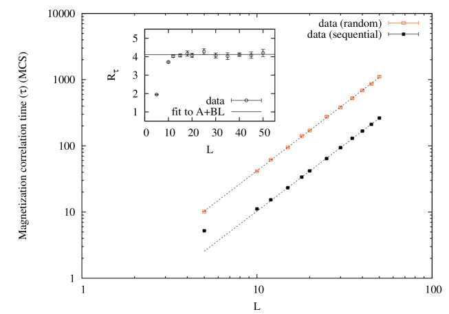
Figure 4: (Color online) Log-log plots of the magnetization correlation times versus $L$ for (a) $x=0\%$ and (b) $x=6\%$. The dashed lines are fits using Eq. (20). Each inset is a plot of the ratio between random and sequential correlation times versus $L$ for the respective ruthenium concentration where the solid line is a fit using $R_{\tau}=A+BL$. All fits were done for $L\geq 15$, to avoid the systematic error introduced by numerical integration, present for correlation times smaller than or equal to 10 MCS, as discussed in Sec. III.

In Fig. 4, we present fits for the correlation times. We note that the curves for both random and sequential correlation times have almost the same slope, which indicates that random and sequential algorithms have approximately the same dynamic exponent $z$, as expected. However, random correlation times are always larger than sequential ones for a fixed system size. In fact we also plot the ratio

$$R_{\tau}=\frac{\tau_{\mbox{\scriptsize{}}}}{\tau_{\mbox{\scriptsize{}}}}$$ (21)

as a function of $L$ and find an almost-constant $R_{\tau}\approx 4$, as shown in the insets of Figs. 4 (a) and 4 (b). For $L\geq 15$, we have fit the data to $R_{\tau}=A+BL$ and obtained $A=4.11(8)$, $B=0.000(3)$ for the pure case and $A=3.8(2)$, $B=0.003(6)$ for the disordered case.

The estimates we get for the dynamical exponent for the pure case are $z=2.02(1)$ for random updates and $z=2.01(1)$ for sequential updates. For the disordered case we have only estimated $z$ for $x=6\%$, which gave us the figures $z=2.06(3)$ and $z=2.02(2)$ for the random and sequential update dynamics, respectively. All values are in agreement with the MC result, $z=2.04(3)$, for the three-dimensional (3D) pure Ising model, presented in Ref. artigo:landau-z, . So, within error bars, both pure and disordered systems have the same dynamic exponent for random or sequential updates. However, we find that the correlation times for a given system size $L$ are always greater for the random update scheme. Therefore, the sequential update version is more efficient than the random update version.

V.3 Critical exponents

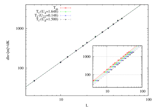
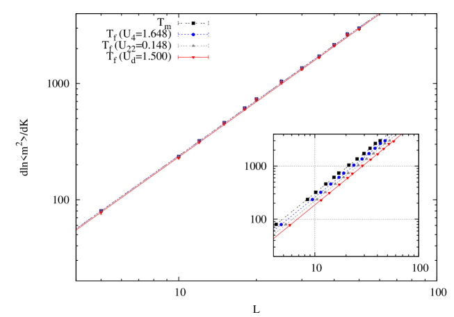
Figure 5: (Color online) Log-log plot of the derivative $dG/dK$ versus $L$ for $x=4\%$, for (a) $G=\ln{\langle|m|\rangle}$ and (b) $G=\ln{\langle m^{2}\rangle}$ [see Eq. (18) and remarks after it]. The data were computed at slightly different critical point estimates, given by the temperatures $T_{m}$ (maximum of $dG/dK$) and $T_{f}$, in order to compare the estimates. The solid lines are fits to $dG/dK=a_{0}L^{1/\nu}$. The inset corresponds to the same graph made with both data and lines slightly shifted along the $L$ axis to make them visible.

Figure 5 shows the comparison between the behavior of some quantities $dG/dK$ at different estimates of the critical point, obtained by the methods described in Sec. IV. Note how the quantities assume almost the same value for the same size at the four different $T_{c}$ estimates. Therefore, the four different fits for each quantity are almost indistinguishable. As a result, the numerical values we obtain for each critical exponent by independent methods are the same, within error bars. Thus, we combine both $T_{m}$ and $T_{f}$ FSS methods to obtain our final estimates of $\alpha$, $\gamma$, $\beta$, and $\nu$ for the disordered systems.

Table 2: Estimates of $1/\nu$ using Eq. (18) for some quantities $G$, with $L_{\mbox{\scriptsize{min}}}=15$. The region $0.30\leq\omega\leq 0.36$ minimized the values of $\chi^{2}/\mbox{DOF}$. In this interval we found no difference between $\chi^{2}/\mbox{DOF}$ up to the second decimal figure for each quantity considered. The values obtained were $\chi^{2}/\mbox{DOF}=0.22$, $0.23$, and $0.081$ for $G=\ln{\langle|m|\rangle}$, $G=\ln{\langle m^{2}\rangle}$, and $G=U$, respectively.

	$1/\nu$
$\omega$	$G=\ln{\langle|m|\rangle}$	$G=\ln{\langle m^{2}\rangle}$	$G=U$
0.300	1.465(31)	1.463(29)	1.444(47)
0.305	1.466(31)	1.464(29)	1.445(46)
0.310	1.467(31)	1.465(29)	1.446(46)
0.315	1.468(31)	1.466(29)	1.448(46)
0.320	1.469(31)	1.467(28)	1.448(46)
0.325	1.470(30)	1.468(28)	1.449(45)
0.330	1.471(30)	1.469(28)	1.450(45)
0.335	1.472(30)	1.470(28)	1.451(45)
0.340	1.473(30)	1.471(28)	1.452(45)
0.345	1.474(30)	1.472(28)	1.453(44)
0.350	1.474(30)	1.473(27)	1.454(44)
0.355	1.475(29)	1.474(27)	1.455(44)
0.360	1.476(29)	1.474(27)	1.456(44)

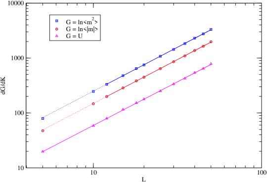
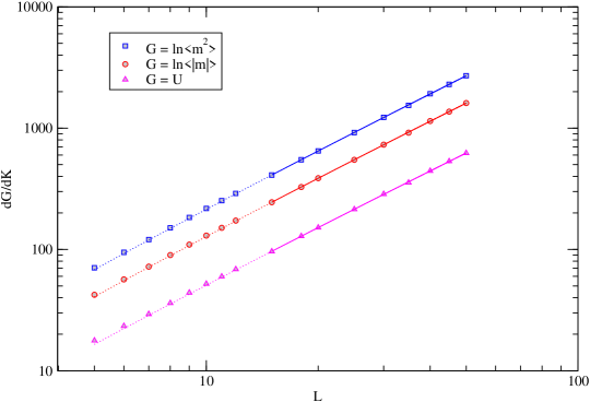
Figure 6: (Color online) Log-log plots of the maxima of some thermodynamic quantities $G$ as functions of $L$ that were used to determine $\nu$ for (a) $x=0\%$ and (b) $x=6\%$. The full lines are fits performed with Eq. (18) for $L_{\mbox{\scriptsize{min}}}<L<50$. The dotted lines are extrapolations of the fits for $L<L_{\mbox{\scriptsize{min}}}$.

To estimate $\nu$ we fit the data to Eq. (18), where we used $G=U$, $G=\ln{\langle|m|\rangle}$, and $G=\ln{\langle m^{2}\rangle}$. For $x=0\%$ we computed the derivatives at the temperature $T_{m}$ where we found the maximum of each quantity. Following the procedure described in Sec. IV, we found good fits with $L_{\mbox{\scriptsize{min}}}=12$ for the logarithmic derivatives and $L_{\mbox{\scriptsize{min}}}=5$ for the Binder’s cumulant. The fits in Fig. 6 (a) were done with $\omega\approx 1.0$, consistent with the result reported in Ref. artigo:landau, . The value we obtain in this work, $\nu=0.6269(20)$, is in excellent agreement with others in the literature for the three-dimensional Ising model artigo:landau ; compostrini1999 ; artigo:butera ; guillou-zinn1980 ; guillou-zinn1987 ; belanger2000 .

For the disordered cases, fits using Eq. (18) were done with the same quantities $G=U$, $G=\ln{\langle|m|\rangle}$, and $G=\ln{\langle m^{2}\rangle}$. Tab. 2 shows our results for $1/\nu$ for $x=6$ $\%$, obtained from data at temperatures $T_{m}$. One of these fits is shown in Fig. 6 (b). Combining the various estimates in Tab. 2, we find $1/\nu=1.4632(90)$ or $\nu=0.6834(42)$. Using both $T_{m}$ and $T_{f}$ methods, we arrive at our final estimate, $\nu=0.6826(46)$, presented in Tab. 3 along with our final estimates of $\nu$ for the other Ru concentrations.

Table 3: Our estimates of the exponents $\alpha$, $\beta$, $\gamma$, and $\nu$ compared to other works in the literature. The lines with the labels $x=0\%$, $4\%$, $6\%$, and $8\%$ correspond to our final estimates. The table also contains other Monte Carlo artigo:landau ; compostrini1999 , high-temperature series expansionartigo:butera , and quantum field theory guillou-zinn1980 ; guillou-zinn1987 results for the pure 3D Ising universality class, as well as Monte Carlo results for the RSIM ballesteros1998 , RBIM calabrese2003tdr ; hasenbusch2007uc , and $\pm J$ Ising Model hasenbusch2007+-J . Reference belanger2000, reports experimental results for both pure and disordered (with low disorder) 3D Ising universality classes.

Pure
	$\alpha$	$\beta$	$\gamma$	$\nu$	$\alpha+2\beta+\gamma$	$2-\alpha-3\nu$
$x=0\%$	0.1093(47)	0.3316(86)	1.2448(70)	0.6269(20)	2.017(29)	0.010(11)
artigo:landau	0.1190(60)	0.3258(44)	1.2390(71)	0.627(2)	2.020(21)	$\equiv 0$
compostrini1999	0.1099(7)	0.32648(18)	1.2371(4)	0.63002(23)	$\equiv 2$	$\equiv 0$
artigo:butera	0.1094(45)	0.3266(10)	1.2375(6)	0.6302(4)	$\equiv 2$	$\equiv 0$
guillou-zinn1980 ; guillou-zinn1987	0.1100(45)	0.3270(15)	1.2390(25)	0.6300(15)	2.003(10)	$\equiv 0$
belanger2000	0.110(5)	0.325(5)	1.25(2)	0.64(1)	2.01(4)	-0.03(4)
Disordered
	$\alpha$	$\beta$	$\gamma$	$\nu$	$\alpha+2\beta+\gamma$	$2-\alpha-3\nu$
$x=4\%$	-0.062(25)	0.3584(96)	1.334(20)	0.6873(84)	1.989(64)	$\equiv 0$
$x=6\%$	-0.049(15)	0.359(16)	1.330(18)	0.6826(46)	1.999(65)	$\equiv 0$
$x=8\%$	-0.057(20)	0.3588(81)	1.337(21)	0.6856(66)	2.003(46)	$\equiv 0$
ballesteros1998	-0.051(16)	0.3546(28)	1.342(10)	0.6837(53)	1.994(32)	0.006(32)
calabrese2003tdr	-0.049(9)	0.3535(17)	1.342(6)	0.683(3)	$\equiv 2$	$\equiv 0$
hasenbusch2007uc	-0.049(6)	0.354(1)	1.341(4)	0.683(2)	$\equiv 2$	$\equiv 0$
hasenbusch2007+-J	-0.046(6)	0.329(2)	1.339(7)	0.682(2)	1.951(17)	$\equiv 0$
belanger2000	-0.10(2)	0.350(9)	1.31(3)	0.69(1)	1.91(7)	0.03(5)

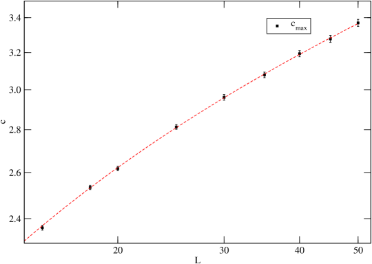
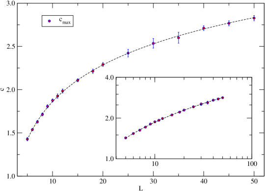
Figure 7: (Color online) Maxima of the specific heat versus $L$. For $x=0\%$ (a), the plot is in log-log scale and the dashed line is a fit of the data using Eq. (17), with $\omega=1.0$. For $x=6\%$ (b), the plot is on a linear scale and the inset corresponds to the same data on a log-log scale. The dashed line in (b) is only a guide to the eye.

Following the same procedures, we used Eq. (17) to find $\alpha$. For $x=0\%$, the results are presented in Tab. 3 and compared to other results in the literature. Figure 7 (a) shows one of the fits for the specific heat of the pure system: we obtain the estimate $\alpha/\nu=0.1743(70)$. For the disordered systems, however, no stable fits were possible with only one correction-to-scaling exponent and we lack statistical resolution to perform fits with higher-order correction-to-scaling terms. Fig. 7 (b) shows one of the plots for the specific heat of the disordered system ($x=6\%$) in which the dashed line is only a guide to the eye.

The estimates for $\alpha$ for the disordered case, presented in Tab. 3, were not determined independently, but were obtained using the Josephson equality $\alpha=2-\nu d$, where $d$ is the dimension ($d=3$ in our case). The $\beta$ and $\gamma$ values were all obtained independently by fitting Eqs. (15) and (16), respectively, and our final estimates are presented in Tab. 3. We see that, within error bars, critical exponents do not depend on the concentration $x$, as expected. Note that the usual scaling relations for the exponents are satisfied, for both pure and disordered cases. This result is an independent check of our calculation. Also, our results for the critical exponents agree, within error bars, with values reported previously elsewhere, obtained both from theoretical methods or from experimental studies. This gives support to our hypothesis concerning the universality class of the model treated in this work.

V.4 Critical temperatures

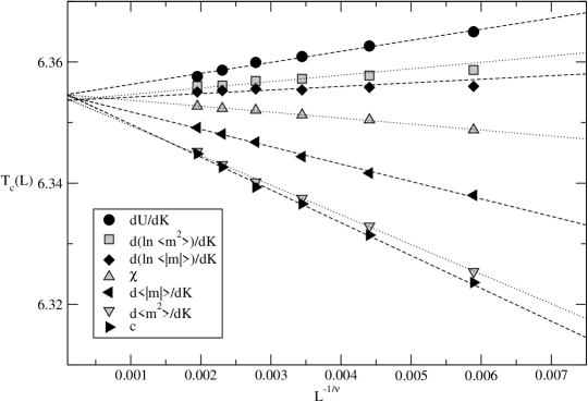
Figure 8: Effective critical temperatures $T_{c}(L)$ versus $L^{-1/\nu}$ estimated for several quantities. The dotted and dashed lines are fits performed with Eq. 19 and using our estimate $\nu=0.6269$.

For $x=0\%$, we fit Eq. (19) for the temperatures where we located peaks of several thermodynamic quantities. Figure 8 shows the values of $T_{m}$ used in our FSS analysis. Our best fits were obtained with $L_{\mbox{\scriptsize{min}}}=25$ for the magnetic susceptibility and the derivatives of $\langle|m|\rangle$ and $U$ and $L_{\mbox{\scriptsize{min}}}=20$ for the remaining quantities. Combining the estimates obtained in those fits, presented in Tab. 4, we obtain: $\bar{T}_{c}=6.3544(6)$, or $K_{c}=0.15737(1)$, which is in excellent agreement with $K_{c}^{\mbox{\scriptsize{}}}=0.1573725(6)$ artigo:butera and with another Monte Carlo evaluation lundow2009 , $K_{c}=0.157371(1)$. We can use our $\bar{T}_{c}$ to estimate the exchange integral of the Fe-Fe bond, $J_{\mbox{\scriptsize{}}}\equiv J$, just by combining the experimental $T_{c}$ in Tab. 1 with the definition $\bar{T}=k_{B}T/J$. We obtain $J=14.16$ meV, which is close to $12.9$ meV, reported in Ref. nilton:feru, and in the interval 10 to 50 meV, as expected for Fe, Co, and Ni kaul1983 .

Table 4: Estimates of $T_{c}(x=0\%)$ obtained with FSS analysis of $T_{c}(L)$ for some thermodynamic quantities.

Quantity	$L_{\mbox{\scriptsize{min}}}$	$\bar{T}_{c}$
$c$	20	6.35514(34)
$\chi$	25	6.35467(11)
$\frac{dU}{dK}$	25	6.35447(37)
$\frac{d\langle|m|\rangle}{dK}$	25	6.35465(34)
$\frac{d}{dK}\ln{\langle|m|\rangle}$	20	6.35360(57)
$\frac{d\langle m^{2}\rangle}{dK}$	20	6.35437(26)
$\frac{d}{dK}\ln{\langle m^{2}\rangle}$	20	6.35359(58)

Table 5: Our Monte Carlo estimates of critical temperatures compared to experimental and mean-field results.

	This work		Experimental artigo:paduani	Mean-field nilton:feru
$x$	$\bar{T}_{c}$	$T_{c}(K)$	$T_{c}(K)$	$T_{c}(K)$
$0\%$	6.3544(6)	-	1043	1043
$2\%$	-	-	968(2)	983
$4\%$	6.1089(23)	1002.7(4)	928(2)	933
$6\%$	5.9615(17)	978.5(3)	908(2)	893
$8\%$	5.8064(22)	953.0(4)	-	863
$10\%$	-	-	838(2)	842

Following the same procedure for the disordered systems and also including the temperatures $T_{f}$ (fixed values of the cumulants) in the analysis, we find the critical temperatures for $x=4\%$, $6\%$, and $8\%$. The value $J=14.16$ meV is used to calculate all critical temperatures in Kelvin, in order to compare with experimental results, as presented in Tab. 5. The mean-field critical temperatures are easily computed with Eq. (2), which is taken from Ref. nilton:feru, [see Eq. (14) in Ref. nilton:feru, ].

Our Monte Carlo estimates of $T_{c}$ for the disordered cases do not agree with the mean-field prediction; neither do they agree with the experimental values. We ascribe this discrepancy to the method by which the parameters of the model were obtained. Although those parameters fit the experimental data well in the mean-field approach, the model is not suitable for these Fe_1-xRu_x alloys in the context of Monte Carlo simulations.

VI Conclusion

In this study we used Monte Carlo simulations to investigate the magnetic properties and critical behavior of a model proposed by Paduani and Branco (2008) for Fe_1-xRu_x alloys through a mean-field approach. Our simulations were restricted to ruthenium concentrations $x=0\%$, $4\%$, $6\%$, and $8\%$. We employed re-weighting single and multiple histogram methods and finite-size scaling analysis, considering up to the first-order correction-to-scaling exponent in order to obtain the critical temperature and critical exponents of the model.

In the pure case, $x=0\%$, the values ​​obtained for the critical exponents are in excellent agreement with the ones in the literature. The critical temperature we found for the pure system also agrees very well with the high-temperature series expansion estimate by Butera and Comi (2000) and with another Monte Carlo result lundow2009 . In the disordered cases, we show that the critical exponents are consistent with the universality class of the transition line between paramagnetic and ferromagnetic phases of three-dimensional Ising models with random site or random bond dilution, as well as with the three-dimensional Ising model with randomly distributed $+J$ and $-J$ exchange integrals.

For $x=4\%$, $6\%$, and $8\%$, our estimates of $T_{c}$ do not agree with the mean-field prediction nor with experimental results. This is expected, since the model parameters were determined through a fitting procedure of experimental data in a mean-field approach nilton:feru . However, the model proposed in Ref. nilton:feru, is in the universality class of three-dimensional disordered Ising models. Furthermore, our values for the critical exponents do not depend on $x$, as expected. This result is obtained only if we take into account a correction-to-scaling term in the finite-size-scaling analysis.

To propose a model that brings simulations and experimental results closer together, we must seek other ways to determine the dependence of the exchange integrals of Fe-Ru and Ru-Ru bonds with the ruthenium concentration. One possibility would be a mean-field renormalization group approach, which is presently being carried out.

- (1) C. Paduani and N. S. Branco, Journal of Physics Condensed Matter 20, 215201 (2008)
- (2) W. Pöttker, C. Paduani, J. Ardisson, and M. Ioshida, Phys. Stat. Sol. B 241, 2586 (2004)
- (3) R. Kikuchi, J. Sanchez, D. De Fontaine, and H. Yamauchi, Acta Metallurgica 28, 651 (1980)
- (4) J. Cardy, Scaling and Renormalization in Statistical Physics (Cambridge University Press, Cambridge, UK, 1996)
- (5) D. Belanger, Braz. J. Phys. 30, 682 (2000)
- (6) M. Hasenbusch, F. Toldin, A. Pelissetto, and E. Vicari, J. Stat. Mech. 2007, P02016 (2007)
- (7) M. E. J. Newman and G. T. Barkema, Monte Carlo Methods in Statistical Physics (Oxford University Press, New York, USA, 1999)
- (8) H. G. Ballesteros, L. A. Fernández, V. Martín-Mayor, A. Muñoz Sudupe, G. Parisi, and J. J. Ruiz-Lorenzo, Phys. Rev. B 58, 2740 (1998)
- (9) P. Calabrese, V. Martín-Mayor, A. Pelissetto, and E. Vicari, Phys. Rev. E 68, 36136 (2003)
- (10) M. Hasenbusch, F. Toldin, A. Pelissetto, and E. Vicari, Phys. Rev. B 76, 94402 (2007)
- (11) H. B. Callen, Thermodynamics and an Introduction to Thermostatistics (John Wiley & Sons, New York, USA, 1985)
- (12) J. Yeomans, Statistcal Mechanics of Phase Transtions (Clarendon Press, New York, USA, 1992)
- (13) N. Metropolis, A. Rosenbluth, M. Rosenbluth, A. Teller, and E. Teller, J. Chem. Phys. 21, 1087 (1953)
- (14) S. Kirkpatrick, J. Comput. Phys. 40, 517 (1981)
- (15) A. M. Ferrenberg and D. P. Landau, Phys. Rev. B 44, 5081 (1991)
- (16) S.-H. Tsai, private communication (2008)
- (17) K. E. Atkinson, An Introduction to Numerical Analysis, 2nd ed. (John Wiley & Sons, New York, USA, 1989) ISBN 9780471500230
- (18) A. M. Ferrenberg and R. H. Swendsen, Phys. Rev. Lett. 61, 2635 (1988)
- (19) A. M. Ferrenberg and R. H. Swendsen, Phys. Rev. Lett. 63, 1195 (1989)
- (20) P. Butera and M. Comi, Phys. Rev. B 62, 14837 (2000)
- (21) P. M. C. de Oliveira, Computing Boolean Statistical Models (World Scientific, Singapore, 1991)
- (22) S. Wansleben and D. Landau, Physical Review B 43, 6006 (1991)
- (23) M. Campostrini, A. Pelissetto, P. Rossi, and E. Vicari, Phys. Rev. E 60, 3526 (1999)
- (24) J. C. Le Guillou and J. Zinn-Justin, Phys. Rev. B 21, 3976 (1980)
- (25) J. C. Le Guillou and J. Zinn-Justin, Journal de Physique 48, 19 (1987)
- (26) P. Lundow, K. Markström, and A. Rosengren, Philosophical Magazine 89, 2009 (2009)
- (27) S. Kaul, Phys. Rev. B 27, 6923 (1983)