Enstrophy growth in the viscous Burgers equation

Abstract

We study bounds on the enstrophy growth for solutions of the viscous Burgers equation on the unit circle. Using the variational formulation of Lu and Doering, we prove that the maximizer of the enstrophy’s rate of change is sharp in the limit of large enstrophy up to a numerical constant but does not saturate the Poincaré inequality for mean-zero $1$-periodic functions. Using the dynamical system methods, we give an asymptotic representation of the maximizer in the limit of large enstrophy as a viscous shock on the background of a linear rarefactive wave. This asymptotic construction is used to prove that a larger growth of enstrophy can be achieved when the initial data to the viscous Burgers equation saturates the Poincaré inequality up to a numerical constant.

An exact self-similar solution of the Burgers equation is constructed to describe formation of a metastable viscous shock on the background of a linear rarefactive wave. When we consider the Burgers equation on an infinite line subject to the nonzero (shock-type) boundary conditions, we prove that the maximum enstrophy achieved in the time evolution is scaled as $\mathcal{E}^{3/2}$, where $\mathcal{E}$ is the large initial enstrophy, whereas the time needed for reaching the maximal enstrophy is scaled as $\mathcal{E}^{-1/2}\log(\mathcal{E})$. Similar but slower rates are proved on the unit circle.

1 Introduction

We consider the initial-value problem for the one-dimensional viscous Burgers equation,

$$\left\{\begin{array}[]{l}u_{t}+2uu_{x}=u_{xx},\;\;\;x\in\mathbb{T},\;t\in\mathbb{R}_{+},\\ u|_{t=0}=u_{0},\phantom{texttext}x\in\mathbb{T},\end{array}\right.$$ (1.1)

where $\mathbb{T}=\left[-\frac{1}{2},\frac{1}{2}\right]$ is the unit circle equipped with the periodic boundary conditions for the real-valued function $u$. Local well-posedness of the initial-value problem (1.1) holds for $u_{0}\in H^{s}_{\rm per}(\mathbb{T})$ with $s>-\frac{1}{2}$ [8]. The Burgers equation is used as a toy model in the context of a bigger problem of how to control existence and regularity of solutions of the three-dimensional Navier–Stokes equations [6, 14]. Recent applications of the Burgers equation to the theory of turbulence can be found in [17, 20].

Lu and Doering [15] considered the question of optimal bounds on the enstrophy growth. The enstrophy for the Burgers equation (1.1) is defined by

$$E(u)=\frac{1}{2}\int_{\mathbb{T}}u_{x}^{2}dx.$$ (1.2)

Integration by parts for a strong local solution of the Burgers equation (1.1) in $H^{3}_{\rm per}(\mathbb{T})$ yields

$$\frac{dE(u)}{dt}=\int_{\mathbb{T}}u_{x}(u_{xxx}-2uu_{xx}-2u_{x}^{2})dx=-\int_{\mathbb{T}}(u_{xx}^{2}+u_{x}^{3})dx\equiv R(u),$$ (1.3)

where $R(u)$ is the rate of change of $E(u)$.

If $u\in{\cal C}_{\rm per}^{1}(\mathbb{T})$, then there is $\xi\in\mathbb{T}$ such that $u_{x}(\xi)=0$. Using the elementary bound,

$$u_{x}^{2}(x)=\left(\int_{\xi}^{x}-\int_{x}^{1+\xi}\right)u_{x}u_{xx}dx\quad\Rightarrow\quad\|u_{x}\|_{L^{\infty}}\leq\|u_{x}\|^{1/2}_{L^{2}}\|u_{xx}\|^{1/2}_{L^{2}},$$

and the Young inequality for $a,b\in\mathbb{R}_{+}$,

$$ab\leq\frac{a^{p}}{p\epsilon^{p}}+\frac{\epsilon^{q}b^{q}}{q},\quad\frac{1}{p}+\frac{1}{q}=1,\quad\epsilon>0,$$

the rate of change $R(u)$ in (1.3) can be estimated by

$$|R(u)|\leq-\|u_{xx}\|_{L^{2}}^{2}+\|u_{x}\|_{L^{2}}^{5/2}\|u_{xx}\|_{L^{2}}^{1/2}\leq\frac{3}{4^{4/3}}\|u_{x}\|_{L^{2}}^{10/3}\equiv\frac{3}{2}E^{5/3}(u),$$ (1.4)

provided that $p=\frac{4}{3}$, $q=4$, and $\epsilon=\sqrt{2}$.

In the framework of the Burgers equation (1.1), Lu and Doering [15] showed that the bound $|R(u)|\leq CE^{5/3}(u)$ on the enstrophy growth is sharp in the limit of large enstrophy, up to a choice of the numerical constant $C>0$. To prove the claim, they considered the maximization problem,

$$\max_{u\in H^{2}_{\rm per}(\mathbb{T})}R(u)\quad\mbox{\rm subject to}\quad E(u)={\cal E},$$ (1.5)

for a given value of ${\cal E}>0$. An analytical solution of the constrained maximization problem (1.5) was studied in the asymptotic limit of large ${\cal E}$ by using Jacobi’s elliptic functions. We note that the bound (1.4) is achieved instantaneously in time and it may not hold for solutions of the viscous Burgers equation (1.1) for a finite time interval.

Ayala and Protas [2] reiterated the same question on the validity of bound (1.4) integrated over a finite time interval. The energy balance equation for the Burgers equation (1.1) is given by

$$K(u)=\frac{1}{2}\int_{\mathbb{T}}u^{2}dx\quad\Rightarrow\quad\frac{dK(u)}{dt}=\int_{\mathbb{T}}u(u_{xx}-2uu_{x})dx=-2E(u).$$ (1.6)

If bound (1.4) is sharp on the time interval $[0,T]$ for some $T>0$, then integration of the enstrophy equation (1.3) implies

$$E^{1/3}(u(T))-E^{1/3}(u_{0})\leq\frac{1}{2}\int_{0}^{T}E(u(t))dt=\frac{1}{4}\left[K(u_{0})-K(u(T))\right].$$ (1.7)

The Burgers equation (1.1) maps the set of periodic functions with zero mean to itself. Using the Poincaré inequality for periodic functions with zero mean,

$$K(u_{0})\leq\frac{1}{4\pi^{2}}E(u_{0}),$$ (1.8)

and neglecting $K(u(T))$ in (1.7), we can obtain

$$E(u(T))\leq\left(E^{1/3}(u_{0})+\frac{1}{16\pi^{2}}E(u_{0})\right)^{3}.$$ (1.9)

Note that this bound together with the monotonicity of $K(u(t))\leq K(u_{0})$ implies global well-posedness of the initial-value problem (1.1) for any $u_{0}\in H^{1}_{\rm per}(\mathbb{T})$.

Using the extended maximization problem for the global solution of the Burgers equation (1.1) in $H^{1}_{\rm per}(\mathbb{T})$,

$$\max_{u_{0}\in H^{1}_{\rm per}(\mathbb{T})}E(u(T))\quad\mbox{\rm subject to}\quad E(u_{0})={\cal E},$$ (1.10)

Ayala and Protas [2] showed numerically that the integral bound (1.9) is not sharp even in the limit of large ${\cal E}$.

We shall use the notation $A=\mathcal{O}({\cal E}^{p})$ as $\mathcal{E}\to\infty$ if there are constants $C_{\pm}$ such that $0\leq C_{-}<C_{+}<\infty$ and $C_{-}\mathcal{E}^{p}\leq A\leq C_{+}\mathcal{E}^{p}$. Let $T_{*}$ be the value of $T$, where $\max_{u_{0}\in H^{1}_{\rm per}(\mathbb{T})}E(u(T))$ is maximal over $T\in\mathbb{R}_{+}$. The main claims in [2] are reproduced in Table I.

Initial condition	Time $T_{*}$	Enstrophy at $T_{*}$	Energy $K$ at $T_{*}$
A maximizer of (1.5)	${\cal O}({\cal E}^{-0.6})$	${\cal O}({\cal E}^{1.0})$	${\cal O}({\cal E}^{0.7})$
A maximizer of (1.10)	${\cal O}({\cal E}^{-0.5})$	${\cal O}({\cal E}^{1.5})$	${\cal O}({\cal E}^{1.0})$

Table I: Enstrophy growth in the Burgers equation from the numerical results in [2].

The first line in Table I shows that the instantaneous maximizer of the problem (1.5) does not saturate the Poincaré inequality (1.8) and does not lead to large growth of the enstrophy. On the other hand, the second line in Table I shows that the bound (1.9) is not sharp. The bound (1.7) could be sharp if $K(u_{0})-K(u(T_{*}))={\cal O}({\cal E}^{1/2})$ but the numerical work in [2] reported large deviations in numerical approximations of this quantity,

$$K(u_{0})-K(u(T_{*}))=\mathcal{O}({\cal E}^{0.68\pm 0.25}),$$ (1.11)

which may indicate that the underlying relation may have a logarithmic (or other) correction.

In this paper, we shall study further properties of the analytical solution of the constrained maximization problem (1.5). We shall use this solution and its generalizations (see Section 2) as an initial condition for the Burgers equation (1.1). In particular, we shall address rigorously the numerical results of [2]. Our main results are summarized in Table II.

Initial condition	Time $T_{*}$	Enstrophy at $T_{*}$	Energy $K$ at $T_{*}$
(2.6) and (2.8)	${\cal O}({\cal E}^{-2/3}\log(\mathcal{E}))$	${\cal O}({\cal E})$	${\cal O}({\cal E}^{2/3})$
(2.6) and (2.9)	${\cal O}({\cal E}^{-1/2}\log^{1/2}(\mathcal{E}))$	${\cal O}({\cal E}^{3/2}\log^{-3/2}(\mathcal{E}))$	${\cal O}({\cal E}\log^{-1}(\mathcal{E}))$

Table II: Enstrophy growth in the Burgers equation from our analytical results.

The analytical results in Table II justify partially the results of numerical approximations in Table I. We conjecture that the optimal rate is achieved with

$$T_{*}={\cal O}({\cal E}^{-1/2}),\quad E(u(T_{*}))={\cal O}({\cal E}^{3/2}),\quad K(u(T_{*}))={\cal O}({\cal E}),$$ (1.12)

but we have no proof of this rate at the present time, perhaps, due to technical limitations of our method (see Remarks 2 and 3). Similarly, we cannot derive an analytical analogue of the numerical result (1.11) and hence, the sharpness of the nonlocal bound (1.7) remains an open question for further studies.

From a technical point of view, using the dynamical system methods, we prove that the maximizer of the constrained maximization problem (1.5) does not saturate the Poincaré inequality (1.8). In the limit of large enstrophy ${\cal E}$, this maximizer resembles a viscous shock on the background of a linear rarefactive wave. If this maximizer is taken as the initial data to the viscous Burgers equation (1.1), it does not give the largest change of enstrophy, compared to the case when the initial data saturates the Poincaré inequality (1.8). On the other hand, if the shock’s width is used as an independent parameter relative to the background intensity of the linear rarefactive wave, the initial data can saturate the Poincaré inequality (1.8) for large values of $\mathcal{E}$, up to a numerical constant, and achieve a faster growth of enstrophy in the time evolution of the viscous Burgers equation.

We note that our construction of the viscous shocks on the background of a linear rarefactive wave is similar to the diffusive $N$-waves that appear at the intermediate stages of dynamics of arbitrary initial data in the Burgers equation over an infinite line [13]. However, these metastable states correspond to Gaussian fundamental solutions of the heat equation in self-similar variables [3, 4], whereas our solutions are obtained on a circle of large but finite period after a scaling transformation. Our results still rely on the analysis of the Burgers equation over an infinite line subject to the non-zero (shock-type) boundary conditions, where viscous shocks are known to be asymptotically stable [19, 10, 11, 22].

The technique of this paper does not use much of the Cole–Hopf transformation [7, 12], which is well known to reduce the viscous Burgers equation to the linear heat equation. The transformation is only used in Sections 5 and 6 to reduce technicalities in the convergence analysis for dynamics of viscous shocks in bounded and unbounded domains. At the same time, one can think about other techniques to prove the conjecture (1.12), which explore the Cole–Hopf transformation in more details. In particular, this transformation shows that solutions of the viscous Burgers equation can be studied with the Laplace method for the heat equation. The Laplace method is typically used to recover solutions of the inviscid Burgers equations from solutions of the viscous Burgers equation in the limit of vanishing viscosity (see, e.g., [21, Chapter 2] or [16, Chapter 3]). Note that the limit of vanishing viscosity corresponds to the limit of large enstrophy in the context of our work. There is a promising way to prove the conjecture (1.12) using the Laplace method after the shock of the corresponding inviscid Burgers equation is formed and this task will be the subject of an independent work [9].

The paper is organized as follows. Section 2 presents main results. Solutions of the constrained maximization problem (1.5) are characterized in Section 3. Self-similar solutions of the Burgers equation on the unit circle are considered in Section 4. Section 5 presents analysis of the Burgers equation on an infinite line. Evolution of a viscous shock on the background of a linear rarefactive wave is studied in Section 6. Proofs of the main results for two different initial data in Table II are given in Sections 7 and 8.

2 Main results

We shall first reexamine the solution of the constrained maximization problem (1.5). Unlike the work of Lu and Doering [15], we avoid the use of special functions (the Jacobi elliptic functions) but use dynamical system techniques to study the limit of large enstrophy ${\cal E}$. As a result, we obtain the following theorem. Here $\check{H}^{2}_{\rm per}(\mathbb{T})$ denotes the restriction of $H^{2}_{\rm per}(\mathbb{T})$ to odd functions and $A=\mathcal{O}_{L^{\infty}}(B)$ as $B\to\infty$ indicates that $\|A\|_{L^{\infty}}=\mathcal{O}(B)$.

Theorem 1

For sufficiently large $\mathcal{E}$, there exists a unique solution $u_{*}\in\check{H}^{2}_{\rm per}(\mathbb{T})$ of the constrained maximization problem (1.5) with $u_{*}^{\prime}(0)<0$ satisfying

$$u_{*}(x)=4k(2x-\tanh(kx))+\mathcal{O}_{L^{\infty}}(k^{2}e^{-k}),\quad\mbox{\rm as}\quad k\to\infty,$$ (2.1)

where $k$ determines the leading order expansions,

$$K(u_{*}) = \frac{8}{3}k^{2}+\mathcal{O}(k),$$ (2.2)

$$E(u_{*}) = \frac{32}{3}k^{3}+\mathcal{O}(k^{2}),$$ (2.3)

$$R(u_{*}) = \frac{256}{5}k^{5}+\mathcal{O}(k^{4}).$$ (2.4)

Corollary 1

When $k$ is expressed from (2.3) in terms of $\mathcal{E}=E(u_{*})$, we obtain

$$\left.\begin{array}[]{l}K(u_{*})=\frac{1}{6^{1/3}}\mathcal{E}^{2/3}+\mathcal{O}(\mathcal{E}^{1/3}),\\ R(u_{*})=\frac{3^{5/3}}{5\cdot 2^{1/3}}\mathcal{E}^{5/3}+\mathcal{O}(\mathcal{E}^{4/3}),\end{array}\right\}\quad\mbox{\rm as}\quad\mathcal{E}\to\infty.$$ (2.5)

Remark 1

Corollary 1 improves the earlier claims in [2] and in [15] based on numerical and asymptotic computations, respectively. It shows that the Poincare inequality (1.8) is not saturated by the solution of the constrained maximization problem (1.5), whereas the bound $|R(u)|\leq CE^{5/3}(u)$ is sharp up to a choice of the numerical constant $C>0$ with

$$C=\frac{3^{5/3}}{5\cdot 2^{1/3}}<\frac{1}{2}.$$

We shall now consider the time evolution of the Cauchy problem (1.1) with the initial data

$$u_{0}(x)=4k(2x-f(x)),\quad x\in\mathbb{T},$$ (2.6)

where $k>0$ is a free parameter and $f:\mathbb{T}\to\mathbb{R}$ is a fixed function satisfying

$$f\in\mathcal{C}^{1}(\mathbb{T}):\quad f(-x)=-f(x),\;\;f\left(\frac{1}{2}\right)=1.$$ (2.7)

The maximizer of Theorem 1 is represented by (2.1). Neglecting the exponentially small terms as $k\to\infty$, this maximizer can be written in the form (2.6) with

$$f(x)=\frac{\tanh(kx)}{\tanh(k/2)}.$$ (2.8)

We say that the initial data (2.6) with (2.8) represents a shock on the background of a linear rarefactive wave, where the width of the shock is inverse proportional to large parameter $k$.

The maximizer of Theorem 1 does not saturate the Poincaré inequality (1.8) in the limit $k\to\infty$ (Remark 1). To allow more flexibility, we can take the initial data (2.6) in the form,

$$f(x)=\frac{\tanh(lx)}{\tanh(l/2)},$$ (2.9)

where parameter $l>0$ may be independent of the large parameter $k$. Figure 1 shows both functions (2.8) and (2.9) in the initial data (2.6) by dashed and solid lines, respectively. If $k=20$ and $l=5$, the shock in (2.9) is much smoother than the shock in (2.8).

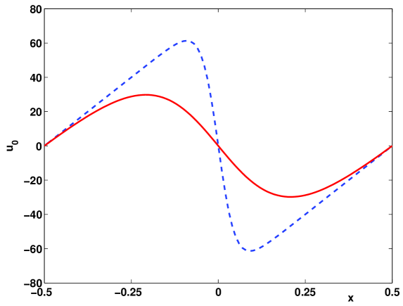
Figure 1: Initial data (2.6) with (2.8) (dotted) or (2.9) (solid) for $k=20$ and $l=5$.

If $u_{0}$ is given by (2.6) with (2.9), then

$$K(u_{0})=k^{2}\tilde{K}(l),\quad E(u_{0})=k^{2}\tilde{E}(l),$$ (2.10)

where

$$\tilde{K}(l) = \frac{32}{3}+\frac{8}{\sinh^{2}(l/2)}-\frac{16\cosh(l/2)}{l\sinh(l/2)}\left[1+\frac{l}{2}+2\log(1+e^{-l})-\frac{2}{l}\int_{0}^{l}\log(1+e^{-z})dz\right],$$

$$\tilde{E}(l) = \frac{32l(\cosh(l)+2)}{3\sinh(l)}-32.$$

If $l=k$, then these expansions yield (2.2) and (2.3) up to the error terms. In this case, if $\mathcal{E}=E(u_{0})$ is fixed, then

$$k=\mathcal{O}(\mathcal{E}^{1/3}),\quad K(u_{0})=\mathcal{O}(\mathcal{E}^{2/3}),\quad\mbox{\rm as}\quad\mathcal{E}\to\infty.$$ (2.11)

The function $F(l)=\tilde{K}(l)/\tilde{E}(l)$ is plotted on Figure 2 (left). We can see that there is a maximum of the function $F$ at $l=l_{0}\approx 3.0$, where the maximum is at

$$F(l_{0})\approx 0.025297<\frac{1}{4\pi^{2}}\approx 0.025330.$$

If $l$ is fixed independently of $k$ and if $\mathcal{E}=E(u_{0})$ is fixed, then

$$k=\mathcal{O}(\mathcal{E}^{1/2}),\quad K(u_{0})=\mathcal{O}(\mathcal{E}),\quad\mbox{\rm as}\quad\mathcal{E}\to\infty.$$ (2.12)

This shows that the initial data (2.6) with (2.9) saturates the Poincaré inequality (1.8) in the limit $k\to\infty$ up to a numerical constant. Note that the value of the constant prefactor $F(l_{0})$ for $l_{0}\approx 3.0$ is $99.9\%$ of the Poincare constant, compared to the numerical computations in [2], where this prefactor was found from solutions of the extended maximization problem (1.10) to be $97\%$ of the Poincare constant.

To apply our method, we shall consider a slow (logarithmic) growth of the parameter $l$ in the limit $k\to\infty$, which yields rates slower than rates (2.12). In particular, we shall use the following elementary result.

Lemma 1

Fix $\Delta>0$ and let $l:=(1+\Delta)\log(k)$. Then, we have

$$k=\mathcal{O}(\mathcal{E}^{1/2}\log^{-1/2}(\mathcal{E})),\quad K(u_{0})=\mathcal{O}(\mathcal{E}\log^{-1}(\mathcal{E})),\quad\mbox{\rm as}\quad\mathcal{E}\to\infty.$$ (2.13)

Proof.

As $k,l\to\infty$, the leading-order expression for $K(u_{0})$ and $E(u_{0})$ are given by

$$K(u_{0})=\frac{8}{3}k^{2}+\mathcal{O}\left(\frac{k^{2}}{l}\right),\quad E(u_{0})=\frac{32}{3}k^{2}l+\mathcal{O}(k^{2}).$$ (2.14)

With the choice of $l:=(1+\Delta)\log(k)$, we are to solve $E(u_{0})=\mathcal{E}$, which is equivalent to the implicit equation,

$$z=x\log(x)+\mathcal{O}(x),\quad z:=\frac{3\mathcal{E}}{16(1+\Delta)},\quad x:=k^{2}.$$ (2.15)

We look at the asymptotic limit $z\to\infty$. Setting

$$x:=\frac{zu}{\log(z)},$$

we rewrite the implicit equation (2.15) as the root finding problem,

$$f(u):=u\left(1-\frac{\log(\log(z))}{\log(z)}+\frac{\log(u)}{\log(z)}+\mathcal{O}\left(\frac{1}{\log(z)}\right)\right)-1=0$$ (2.16)

We note that $f(1)=\mathcal{O}\left(\frac{\log(\log(z))}{\log(z)}\right)\to 0$ as $z\to\infty$ and $f^{\prime}(1)=1+\mathcal{O}\left(\frac{\log(\log(z))}{\log(z)}\right)\neq 0$ as $z\to\infty$. By the implicit function theorem, there is a unique root in the neighborhood of $u=1$ such that $u=1+\mathcal{O}\left(\frac{\log(\log(z))}{\log(z)}\right)$ as $z\to\infty$. The assertion (2.13) holds by (2.14) and (2.15). ∎

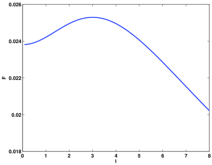
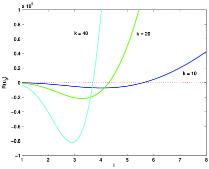
Figure 2: Function $F(l)=\tilde{K}(l)/\tilde{E}(l)$ versus $l$ (left) and function $R(u_{0})$ versus $l$ for different values of $k$ (right).

If $u_{0}$ is given by (2.6) and (2.9), then

$$R(u_{0}) = 64k^{3}\left[16-\frac{12l}{\tanh^{2}(l/2)}\int_{0}^{l/2}{\rm sech}^{4}(x)dx+\frac{2l^{2}}{\tanh^{3}(l/2)}\int_{0}^{l/2}{\rm sech}^{6}(x)dx\right]$$

$$\phantom{texttext}-\frac{128k^{2}l^{3}}{\tanh^{2}(l/2)}\int_{0}^{l/2}\sinh^{2}(x){\rm sech}^{6}(x)dx.$$

The dependence of $R(u_{0})$ versus $l$ for different values of $k$ is shown on Figure 2 (right). Since $R(u_{0})>0$ for large values of $k$ and $l$, the enstrophy $E(u)$ grows initially for $t>0$.

We shall construct a solution of the Burgers equation (1.1) starting with the initial data (2.6)–(2.7). We prove that this solution displays dynamics consisting of two phases. In the first phase, a metastable viscous shock is formed from the function $-4kf(x)$. In the second phase, a rarefactive wave associated with the linear function $8kx$ decays to zero. We compute the growth of enstrophy in two cases: when $l=\mathcal{O}(k)$ and the scaling law (2.11) holds and when $l=\mathcal{O}(\log(k))$ and the scaling law (2.13) holds. The following theorem gives the main result of this paper.

Theorem 2

Consider the initial-value problem (1.1) with initial data in (2.6) and (2.9). Let $\mathcal{E}=E(u_{0})$ be the initial enstrophy. There exists $T_{*}>0$ such that the enstrophy $E(u)$ achieves its maximum at $u_{*}=u(\cdot,T_{*})$. If $l=\mathcal{O}(k)$ as $k\to\infty$, then

$$T_{*}=\mathcal{O}(\mathcal{E}^{-2/3}\log(\mathcal{E})),\quad E(u_{*})=\mathcal{O}(\mathcal{E}),\quad K(u_{*})=\mathcal{O}(\mathcal{E}^{2/3}),\quad\mbox{\rm as}\quad\mathcal{E}\to\infty,$$ (2.17)

whereas if $l=\mathcal{O}(\log(k))$ as $k\to\infty$, then

$$T_{*}=\mathcal{O}(\mathcal{E}^{-1/2}\log^{1/2}(\mathcal{E})),\quad E(u_{*})=\mathcal{O}(\mathcal{E}^{3/2}\log^{-3/2}(\mathcal{E})),\quad K(u_{*})=\mathcal{O}(\mathcal{E}\log^{-1}(\mathcal{E})),$$ (2.18)

as $\mathcal{E}\to\infty$.

Remark 2

Several obstacles appear in our method when we consider the case $l=\mathcal{O}(1)$ and the scaling law (2.12). These obstacles come from the behavior of the solution $u(x,t)$ near the boundaries $x=\pm\frac{1}{2}$ as well as from the constraints on the inertial time interval $[0,T]$, during which the solution approaches the viscous shock on the background of a linear rarefactive wave.

3 Proof of Theorem 1

To prove Theorem 1, we obtain a convenient analytical representation of solutions of the constrained maximization problem (1.5). We set $v=u_{x}$ and look for critical points $v\in H^{1}_{\rm per}(\mathbb{T})$ of the functional,

$$J(v)=\int_{\mathbb{T}}\left(v_{x}^{2}+v^{3}+\lambda v^{2}+\mu v\right)dx,$$ (3.1)

where $\lambda,\mu\in\mathbb{R}$ are the Lagrange multipliers associated with the following constraints,

$$\frac{1}{2}\int_{\mathbb{T}}v^{2}(x)dx={\cal E},\quad\int_{\mathbb{T}}v(x)dx=0.$$ (3.2)

The latter constraint ensures that $u$ is a periodic function on $\mathbb{T}$. If $v$ is even in $H^{1}_{\rm per}(\mathbb{T})$ and has zero mean, then $u(x)=\int_{0}^{x}v(x^{\prime})dx^{\prime}$ is odd in $H^{2}(\mathbb{T})$, $u(\pm 1)=0$, and hence, $u\in\check{H}^{2}_{\rm per}(\mathbb{T})$.

The Euler–Lagrange equations associated with the functional $J(v)$ yield the second-order differential equation,

$$2v^{\prime\prime}(x)=3v^{2}(x)+2\lambda v(x)+\mu,\quad x\in\mathbb{T}.$$ (3.3)

Integrating equation (3.3) over $\mathbb{T}$ and using the constraints (3.2), we find $\mu=-6{\cal E}$. Hence we are dealing with the family of integrable second-order equations,

$$\frac{d^{2}v}{dx^{2}}=\frac{3}{2}v^{2}+\lambda v-3{\cal E}\quad\Rightarrow\quad\left(\frac{dv}{dx}\right)^{2}=v^{3}+\lambda v^{2}-6{\cal E}v+I,$$ (3.4)

where $I$ is an integration constant.

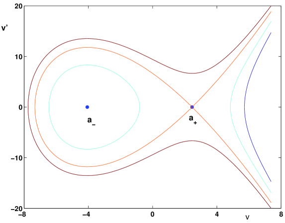
Figure 3: Phase portrait for the Euler–Lagrange equation (3.4) with $\mathcal{E}=5$.

The phase plane of system (3.4) is given by $(v,v^{\prime})\in\mathbb{R}^{2}$. A typical phase portrait is shown on Figure 3. There exist two equilibrium points of the second-order equation (3.4), denoted by $(a_{-},0)$ and $(a_{+},0)$, where

$$a_{\pm}=\frac{1}{3}\left(-\lambda\pm\sqrt{\lambda^{2}+18{\cal E}}\right)\quad\Rightarrow\quad a_{-}<0<a_{+}.$$ (3.5)

Let us define

$$I_{\pm}=-a_{\pm}^{3}-\lambda a_{\pm}^{2}+6{\cal E}a_{\pm}\quad\Rightarrow\quad I_{-}<I_{+}.$$ (3.6)

The equilibrium $(a_{-},0)$ is a center, whereas the equilibrium $(a_{+},0)$ is a saddle point. For $I=I_{+}$, there exists a homoclinic orbit connecting the stable and unstable manifolds of the saddle point $(a_{+},0)$. This orbit can be found analytically,

$$v(x)=a_{+}-4k^{2}{\rm sech}^{2}(kx),\quad k=\frac{1}{2}\sqrt[4]{\lambda^{2}+18{\cal E}}.$$ (3.7)

Inside the separatrix loop, there is a family of $T$-periodic orbits for $I\in(I_{-},I_{+})$, such that $T$ is a strictly increasing function of $I$ with

$$T\to\frac{2\pi}{\omega}\quad\mbox{\rm as}\quad I\to I_{-},\quad\mbox{\rm and}\quad T\to\infty\quad\mbox{\rm as}\quad I\to I_{+},$$ (3.8)

where

$$\omega^{2}=-\lambda-3a_{-}=\sqrt{\lambda^{2}+18{\cal E}}=4k^{2}.$$

If $k>\pi$, there is a unique $I_{0}\in(I_{-},I_{+})$ such that $T=1$ at $I=I_{0}$. The corresponding $1$-periodic solution $v\in H^{1}_{\rm per}(\mathbb{T})$ of equation (3.3) is a critical point of $J(v)$. Integrating (3.4) for $I=I_{0}$ further, we obtain a $1$-periodic solution $v(x-x_{0})$, where $x_{0}\in\mathbb{T}$ is chosen uniquely from the constraints $v^{\prime}(0)=0$ and $v(0)<a_{-}<0$ (which yield an odd $u$ with $u^{\prime}(0)<0$). In this way, a critical point of $J(v)$ is obtained and the parameter $\lambda$ needs to be defined by the constraint $E(u)=\mathcal{E}$.

To satisfy the constraint $E(u)={\cal E}$ and to justify the asymptotic expansion (2.1), we can use the representation,

$$v(x)=a_{+}-4k^{2}y(\xi),\quad\xi=kx,$$ (3.9)

where $y(\xi)$ is a $k$-periodic solution of the second-order equation,

$$y^{\prime\prime}-4y+6y^{2}=0.$$ (3.10)

The $k$-periodic solution of equation (3.10), which is called a cnoidal wave, is equivalent to a $k$-periodic sequence of homoclinic solutions, which are called solitary waves [5] (see also Chapter 3 in [1]). This representation uses the theory of Jacobi’s elliptic functions. We can obtain an equivalent approximation result by using methods of the dynamical system theory [18].

Lemma 2

There are $k_{0}>0$ and $C>0$ such that for all $k\in(k_{0},\infty)$, the $k$-periodic solution $y(\xi)$ of the second-order equation (3.10) is close to the solitary wave $y_{\infty}(\xi)={\rm sech}^{2}(\xi)$ with the error bound,

$$\sup_{\xi\in[-k/2,k/2]}\left|y(\xi)-y_{\infty}(\xi)\right|\leq Ce^{-k}.$$ (3.11)

Proof.

We write a $k$-periodic sequence of the solitary waves as

$$y_{0}(\xi)=\sum_{n\in\mathbb{Z}}{\rm sech}^{2}(\xi+kn)$$

and decompose the solution $y$ of equation (3.10) as $y(\xi)=y_{0}(\xi)+Y(\xi)$. After straightforward computations, $Y$ satisfies

$$LY=F(Y),$$

where $L=-\partial_{\xi}^{2}+4-12{\rm sech}^{2}(\xi)$ and

$$F(Y)=6Y^{2}+12\sum_{n\in\mathbb{Z}\backslash\{0\}}{\rm sech}^{2}(\xi+kn)Y+6\sum_{n\in\mathbb{Z}}\sum_{l\in\mathbb{Z}\backslash\{n\}}{\rm sech}^{2}(\xi+kn){\rm sech}^{2}(\xi+kl).$$

The operator $L:H^{2}(\mathbb{R})\to L^{2}(\mathbb{R})$ has a one-dimensional kernel spanned by the odd function $y_{\infty}^{\prime}(\xi)$. The rest of the spectrum of $L$ includes an isolated eigenvalue at $-5$ and the continuous spectrum for $[4,\infty)$. Hence the operator $L$ is invertible in the space of even functions.

Let $\mathbb{T}_{k}:=\left[-\frac{k}{2},\frac{k}{2}\right]$ and denote the restriction of $H^{2}_{\rm per}(\mathbb{T}_{k})$ to even functions by $\hat{H}^{2}_{\rm per}(\mathbb{T}_{k})$. Let $\hat{L}:\hat{H}^{2}_{\rm per}(\mathbb{T}_{k})\to\hat{L}^{2}_{\rm per}(\mathbb{T}_{k})$ be a restriction of $L$. Then, $\hat{L}$ is invertible if $k$ is sufficiently large, and existence and uniqueness of small solutions $Y\in H^{2}_{\rm per}(\mathbb{T}_{k})$ of the fixed-point problem $Y=\hat{L}^{-1}F(Y)$ can be found by using contraction mapping arguments, provided that

$$\left\|\sum_{n\in\mathbb{Z}\backslash\{0\}}{\rm sech}^{2}(\cdot+kn)\right\|_{L^{\infty}(\mathbb{T}_{k})}\quad\mbox{\rm and}\quad\left\|\sum_{n\in\mathbb{Z}}\sum_{l\in\mathbb{Z}\backslash\{n\}}{\rm sech}^{2}(\cdot+kn){\rm sech}^{2}(\cdot+kl)\right\|_{L^{2}(\mathbb{T}_{k})}$$

converge to zero as $k\to\infty$. We check this by explicit computations. There are $k_{0}>0$ and $C_{1},C_{2}>0$ such that for all $k\in(k_{0},\infty)$, we have

$$\left\|\sum_{n\in\mathbb{Z}\backslash\{0\}}{\rm sech}^{2}(\cdot+kn)\right\|_{L^{\infty}(\mathbb{T}_{k})}\leq\sum_{n\in\mathbb{N}}\frac{8e^{-(2n-1)k}}{(1+e^{-(2n-1)k})^{2}}\leq C_{1}e^{-k}$$ (3.12)

and

$$\left\|\sum_{n\in\mathbb{Z}}\sum_{l\in\mathbb{Z}\backslash\{n\}}{\rm sech}^{2}(\cdot+kn){\rm sech}^{2}(\cdot+kl)\right\|_{L^{2}(\mathbb{T}_{k})}$$ (3.13)

$$\phantom{text}\leq\left\|{\rm sech}^{2}(\cdot)\right\|_{L^{2}(\mathbb{T}_{k})}\left\|\sum_{l\in\mathbb{Z}\backslash\{0\}}{\rm sech}^{2}(\cdot+kl)\right\|_{L^{\infty}(\mathbb{T}_{k})}$$

$$\phantom{texttexttexttexttexttext}+2\sum_{n\in\mathbb{N}}\left\|{\rm sech}^{2}(\cdot+kn)\right\|_{L^{\infty}(\mathbb{T}_{k})}\left\|\sum_{l\in\mathbb{Z}\backslash\{n\}}{\rm sech}^{2}(\cdot+kl)\right\|_{L^{2}(\mathbb{T}_{k})}$$

$$\phantom{text}\leq 3\left\|{\rm sech}^{2}(\cdot)\right\|_{L^{2}(\mathbb{T}_{k})}\left\|\sum_{l\in\mathbb{Z}\backslash\{0\}}{\rm sech}^{2}(\cdot+kl)\right\|_{L^{\infty}(\mathbb{T}_{k})}$$

$$\phantom{texttexttexttexttexttext}+4k^{1/2}\sum_{n\in\mathbb{N}}\sum_{l\in\mathbb{N}}\left\|{\rm sech}^{2}(\cdot+kn)\right\|_{L^{\infty}(\mathbb{T}_{k})}\left\|{\rm sech}^{2}(\cdot+kl)\right\|_{L^{\infty}(\mathbb{T}_{k})}$$

$$\phantom{text}\leq 2\sqrt{3}C_{1}e^{-k}+4C_{1}^{2}k^{1/2}e^{-2k}\leq C_{2}e^{-k}.$$

Existence and uniqueness of $Y$ with the error bound (3.11) follow from bounds (3.12) and (3.13), the contraction mapping arguments for $Y=\hat{L}^{-1}F(Y)$ in $\hat{H}^{2}_{\rm per}(\mathbb{T}_{k})$, and the Sobolev embedding of $H^{2}_{\rm per}(\mathbb{T}_{k})$ to $L^{\infty}_{\rm per}(\mathbb{T}_{k})$. ∎

To define uniquely $\lambda$ in terms of ${\cal E}$, we recall the constraints (3.2), which are equivalent to the scalar equation,

$$a_{+}=4k\int_{-k/2}^{k/2}y(\xi)d\xi=8k(1+{\cal O}(ke^{-k})).$$ (3.14)

Because $a_{+}$ is related to $k$ by the exact expression (3.5), constraint (3.14) yields a relationship between $k$ and ${\cal E}$ given by

$$a_{+}=\frac{6\mathcal{E}}{\lambda+4k^{2}}\quad\Rightarrow\quad 32k^{3}\left(1+\mathcal{O}(ke^{-k})\right)=\frac{6\mathcal{E}}{1+\sqrt{1-\frac{9\mathcal{E}}{8k^{4}}}}.$$ (3.15)

Hence we obtain

$$k=\left(\frac{3}{32}{\cal E}\right)^{1/3}+1+\mathcal{O}(\mathcal{E}^{-1/3})\quad\mbox{\rm as}\quad{\cal E}\to\infty,$$ (3.16)

which yields as $\mathcal{E}\to\infty$,

$$\lambda = 4k^{2}\sqrt{1-\frac{9\mathcal{E}}{8k^{4}}}=\left(\frac{3}{4}{\cal E}\right)^{2/3}+\mathcal{O}(\mathcal{E}^{1/3})$$

and

$$a_{+} = 8k(1+{\cal O}(ke^{-k}))=\left(48{\cal E}\right)^{1/3}+\mathcal{O}(1).$$

It follows from (3.16) that

$$\mathcal{E}=\frac{32}{3}k^{3}-32k^{2}+\mathcal{O}(k),\quad\mbox{\rm as}\quad k\to\infty,$$

which recovers (2.3).

Using constraints (3.2), the Euler–Lagrange equation (3.3), the representation (3.9), and the constraint (3.14), we obtain

$$R(u) = 2\lambda{\cal E}+\frac{1}{2}\int_{\mathbb{T}}v^{3}(x)dx$$ (3.17)

$$= 2\lambda{\cal E}+a_{+}^{2}(4k^{2}-a_{+})-32k^{5}\int_{-k/2}^{k/2}y^{3}(\xi)d\xi.$$

Approximations (3.11), (3.15), and (3.16) in (3.17) yield

$$R(u)=\frac{256}{5}k^{5}+{\cal O}(k^{4})\quad\mbox{\rm as}\quad k\to\infty,$$

which recovers (2.4).

To obtain (2.1) and (2.2), we integrate the solution $v(x)$ and write

$$u(x)=\int_{0}^{x}v(x^{\prime})dx^{\prime}=a_{+}x-4kz(kx),$$ (3.18)

where

$$z(\xi)=\int_{0}^{\xi}y(\xi^{\prime})d\xi^{\prime},\quad\xi=kx.$$

Therefore, we have

$$K(u) = \frac{1}{24}a_{+}^{2}-8ka_{+}\int_{0}^{1/2}xz(kx)dx+8k\int_{-k/2}^{k/2}z^{2}(\xi)d\xi.$$

It follows from (3.11) that for all large $k$, there is $C>0$ such that $z(\xi)$ is close to $z_{\infty}(\xi)=\tanh(\xi)$ with the error bound,

$$\sup_{\xi\in[-k/2,k/2]}\left|z(\xi)-z_{\infty}(\xi)\right|\leq Cke^{-k},$$ (3.19)

which recovers (2.1) thanks to the expansion (3.14).

Integrating by parts, we also find the elementary expansion,

$$\int_{0}^{1/2}x\tanh(kx)dx=\frac{1}{8}+\frac{1}{4k^{2}}\int_{0}^{\infty}\log(1+e^{-z})dz+{\cal O}(k^{-1}e^{-k})\quad\mbox{\rm as}\quad k\to\infty.$$

Together with (3.14) and (3.16), this expansion yields

$$K(u)=\frac{8}{3}k^{2}-16k+32\int_{0}^{\infty}\log(1+e^{-z})dz+{\cal O}(k^{3}e^{-k}))\quad\mbox{\rm as}\quad k\to\infty,$$

which recovers (2.2).

To complete the proof of Theorem 1, we need to show that the critical point $u\in\check{H}^{2}_{\rm per}(\mathbb{T})$ of $J(u_{x})$ is a maximizer of $R(u)$. However, this follows from the uniqueness of the critical point $u_{*}$, for which $R(u_{*})>0$, and from the fact that $R(u)$ is bounded from above by the bound (1.4). Therefore, the proof of Theorem 1 is complete.

4 Burgers equation on the unit circle

To develop the proof of Theorem 2, we convert the initial-value problem for the Burgers equation (1.1) with initial data (2.6)–(2.7) to a convenient form, which separates the decay of the linear rarefactive wave and the relative dynamics of a shock on the background of the rarefactive wave.

Lemma 3

Let $u_{0}$ be given by (2.6)–(2.7). Then, a unique solution $u\in C(\mathbb{R}_{+},H^{1}_{\rm per}(\mathbb{T}))$ of the Burgers equation (1.1) is given by

$$u(x,t)=p(t)\left(2x-w(\xi(x,t),\tau(t))\right),\quad x\in\mathbb{T},\quad t\in\mathbb{R}_{+},$$ (4.1)

where

$$p(t)=\frac{4k}{1+16kt},\quad\xi(x,t)=\frac{4kx}{1+16kt},\quad\tau(t)=\frac{16k^{2}t}{1+16kt},$$ (4.2)

and $w(\xi,\tau)$ is a unique odd solution of the Burgers equation,

$$\left\{\begin{array}[]{l}w_{\tau}=2ww_{\xi}+w_{\xi\xi},\quad\;|\xi|<2(k-\tau),\quad\tau\in(0,k),\\ w|_{\tau=0}=f(\xi/4k),\quad\;\;|\xi|\leq 2k,\end{array}\right.$$ (4.3)

subject to the boundary conditions $w=\pm 1$ at $\xi=\pm 2(k-\tau)$.

Proof.

Although the proof can be constructed by a direct substitution, we will give all intermediate details. Recall that the initial-value problem (1.1) has a unique global solution $u\in C(\mathbb{R}_{+},H^{1}_{\rm per}(\mathbb{T}))$ if the initial data $u_{0}$ satisfies (2.6)–(2.7). Odd solutions in $x$ are preserved in the time evolution of the Burgers equation (1.1) and the Sobolev embedding of $H^{1}_{\rm per}(\mathbb{T})$ to $C_{\rm per}(\mathbb{T})$ implies that the boundary conditions $u(\pm\frac{1}{2},t)=0$ are preserved for all $t>0$.

Let us look for the exact solution of the Burgers equation (1.1) in the separable form,

$$u(x,t)=p(t)\left(2x-U(x,q(t))\right),$$

where $p(t)$, $q(t)$, and $U(x,q)$ are new variables. If we choose $\dot{p}=-4p^{2}$ and $\dot{q}=p$ starting with $p(0)=p_{0}$ and $q(0)=0$, then $U(x,q)$ satisfies the initial-value problem,

$$\left\{\begin{array}[]{l}U_{q}+4xU_{x}=2UU_{x}+\frac{1}{p(t)}U_{xx},\quad x\in\mathbb{T},\quad q>0,\\ U|_{t=0}=f(x),\qquad\phantom{textttext}\qquad x\in\mathbb{T},\end{array}\right.$$ (4.4)

subject to the boundary conditions $U=\pm 1$ at $x=\pm\frac{1}{2}$. In addition, $U$ is odd in $x$ for any $q>0$.

We find from the differential equations $\dot{p}=-4p^{2}$ and $\dot{q}=p$ that

$$p(t)=\frac{p_{0}}{1+4p_{0}t},\quad q(t)=\frac{1}{4}\log(1+4p_{0}t).$$

Solving equation $U_{q}+4xU_{x}=0$ along the characteristics, we define

$$\frac{dx}{dq}=4x\quad\Rightarrow\quad x=Ce^{4q},$$

where $C$ is an integration constant. Noting that $p(t)=p_{0}e^{-4q}$, we define $(\xi,\tau)$ by

$$\frac{\partial\tau}{\partial q}=p_{0}e^{-4q},\quad\frac{\partial\xi}{\partial q}=-4\xi,\quad\frac{\partial\tau}{\partial x}=p_{0}e^{-4q}.$$

Integrating these equations, we obtain the substitution,

$$U(x,q)=w(\xi,\tau),\quad\xi=p_{0}xe^{-4q}=\frac{p_{0}x}{1+4p_{0}t},\quad\tau=\frac{1}{4}p_{0}(1-e^{-4q})=\frac{p_{0}^{2}t}{1+4p_{0}t},$$

which transforms (4.4) to (4.3). Odd functions $U$ in $x$ become odd functions $w$ in $\xi$ and the boundary conditions $U=\pm 1$ at $x=\pm\frac{1}{2}$ become the boundary conditions $w=\pm 1$ at $\xi=\pm\frac{1}{2}(p_{0}-4\tau)$. Setting $p_{0}=4k$ yields (4.1), (4.2), and (4.3). ∎

Remark 3

The scaling law (1.12) formally follows from the similarity transformation (4.1). If there exists an inertial range $C_{-}\leq kt\leq C_{+}$ for some $k$-independent constants $0<C_{-}<C_{+}<\infty$, where the $H^{1}$-norm of $w$ in $\xi$ is $k$-independent, then in this range, $p(t)=\mathcal{O}(k)$, $K(u)=\mathcal{O}(k^{2})$, $E(u)=\mathcal{O}(k^{3})$, where $k=\mathcal{O}(\mathcal{E}^{1/2})$ as $\mathcal{E}=E(u_{0})\to\infty$. To prove this claim rigorously, we study a convergence of solutions of the rescaled Burgers equation (4.3) starting with the initial condition $w_{0}(\xi)=f(\xi/4k)$ to the $k$-independent viscous shock $w_{\infty}(\xi)=\tanh(\xi)$ in a bounded but large domain $|\xi|\leq 2(k-\tau)$ for $\tau=\mathcal{O}(k)$. For a control of error terms, we have to specify further restriction on the initial condition $f(\xi/4k)$, which result in weaker statements (2.17) and (2.18) of Theorem 2.

The Burgers equation $w_{\tau}=2ww_{\xi}+w_{\xi\xi}$ admits the viscous shock,

$$w_{\infty}(\xi)=\tanh(\xi).$$ (4.5)

In the initial-value problem,

$$\left\{\begin{array}[]{l}w_{\tau}=2ww_{\xi}+w_{\xi\xi},\quad\xi\in\mathbb{R},\quad\tau\in\mathbb{R}_{+},\\ w|_{\tau=0}=g(\xi/a),\quad\;\;\;\;\xi\in\mathbb{R},\end{array}\right.$$ (4.6)

where $a>0$ is a parameter, the viscous shock is an asymptotically stable attractor in the space of odd functions $g$ with fast (exponential) decay to $\pm 1$ as $\xi\to\pm\infty$ [10]. To be able to deal with the dynamics of viscous shocks in the initial-value problem (4.3) on a bounded domain, we shall first clarify the dynamics of viscous shocks in the initial-value problem (4.6) on the infinite line.

5 Burgers equation on the infinite line

Let us rewrite the initial-value problem (4.6) for the Burgers equation on the infinite line by using the original (unscaled) variables,

$$\left\{\begin{array}[]{l}u_{t}+2uu_{x}=u_{xx},\quad x\in\mathbb{R},\;\;t\in\mathbb{R}_{+},\\ u|_{t=0}=u_{0},\quad\quad\quad\;\;x\in\mathbb{R},\end{array}\right.$$ (5.1)

We impose the nonzero (shock-type) boundary conditions,

$$\lim_{x\to\pm\infty}u(x,t)=\mp U_{\infty},\quad t\in\mathbb{R}_{+},$$ (5.2)

for some $U_{\infty}>0$.

To control the enstrophy on the infinite line, we define

$$E(u)=\frac{1}{2}\int_{\mathbb{R}}u_{x}^{2}dx,\quad R(u)=-\int_{\mathbb{R}}(u_{xx}^{2}+u_{x}^{3})dx,\quad\frac{dE(u)}{dt}=R(u).$$ (5.3)

The bound $|R(u)|\leq\frac{3}{2}E^{5/3}(u)$ on the enstrophy growth is derived similarly to (1.4). In the case of the infinite line, the maximizer of $R(u)$ at fixed $E(u)$ is not decaying at infinity. On the other hand, the result of Theorem 1 becomes now explicit.

Lemma 4

The maximization problem,

$$\max_{u_{x}\in H^{1}(\mathbb{R})}R(u)\quad\mbox{\rm subject to}\quad E(u)={\cal E},$$ (5.4)

admits a unique odd solution

$$u_{*}(x)=-4k\tanh(kx),$$ (5.5)

where $k$ is defined implicitly by ${\cal E}$,

$${\cal E}=E(u_{*})=\frac{32}{3}k^{3},$$ (5.6)

and

$$R(u_{*})=\frac{256}{5}k^{5}=\frac{3^{5/3}}{5\cdot 2^{1/3}}{\cal E}^{5/3}.$$ (5.7)

Proof.

The constrained maximization problem (5.4) for $v=u_{x}\in H^{1}(\mathbb{R})$ yields the functional,

$$J(v)=\int_{\mathbb{R}}\left(v_{x}^{2}+v^{3}+\lambda v^{2}\right)dx,$$

where $\lambda\in\mathbb{R}$ is the Lagrange multiplier. The Euler–Lagrange equations give

$$2v^{\prime\prime}(x)=3v^{2}(x)+2\lambda v(x),\quad x\in\mathbb{R}$$

for which the only solution $v\in H^{1}(\mathbb{R})$ is the soliton,

$$v(x)=-4k^{2}{\rm sech}^{2}(kx),\quad\lambda=4k^{2},$$

where $k>0$ is arbitrary. Integrating $v(x)$ with respect to $x$, we obtain (5.5). Integrating $v^{2}$, $v^{3}$, and $v_{x}^{2}$ over $\mathbb{R}$, we obtain (5.6) and (5.7). ∎

Remark 4

The Burgers equation (5.1) subject to the boundary conditions (5.2) with $U_{\infty}=4k$ admits the viscous shock solution,

$$u_{\infty}(x)=-4k\tanh(4kx),\quad k>0,$$ (5.8)

which yields $R(u_{\infty})=0$ and $E(u_{\infty})=4E(u_{*})$.

Remark 5

Using the self-similar variables,

$$u(x,t)=-4kw(\xi,\tau),\quad\xi=4kx,\quad\tau=16k^{2}t,$$ (5.9)

the Burgers equation (5.1) can be written in the form,

$$\left\{\begin{array}[]{l}w_{\tau}=2ww_{\xi}+w_{\xi\xi},\quad\xi\in\mathbb{R},\;\;\tau\in\mathbb{R}_{+},\\ w|_{\tau=0}=w_{0},\quad\quad\quad\;\;\xi\in\mathbb{R},\end{array}\right.$$ (5.10)

where $u_{0}(x)=-4kw_{0}(\xi)$. If the boundary conditions (5.2) are imposed with $U_{\infty}=4k$, then $w$ satisfies the boundary conditions $\lim_{\xi\to\pm\infty}w(\xi,\tau)=\pm 1$.

5.1 Initial condition with $l=k$

Let us consider the time evolution of the Burgers equations (5.1) and (5.10) starting with the initial condition,

$$u_{0}(x)=-4k\tanh(kx),\quad\Rightarrow\quad w_{0}(\xi)=\tanh(\xi/4),$$ (5.11)

which is a local maximizer (5.5) in Lemma 5.7. Note that the initial-value problem (5.10) with initial data (5.11) is independent of parameter $k>0$. We shall prove the following.

Lemma 5

For any integer $m\geq 0$, there is a constant $C_{m}>0$ such that a unique solution of the initial-value problem (5.10) with initial data (5.11) satisfies

$$\sup_{\xi\in\mathbb{R}}\left|e^{|\xi|/2}\partial_{\xi}^{m}\left(w(\xi,\tau)-\tanh(\xi)\right)\right|\leq C_{m}e^{-3\tau/4},\quad\tau\in\mathbb{R}_{+}.$$ (5.12)

Proof.

Using the Cole–Hopf transformation [7, 12], the Burgers equation (5.10) with initial data (5.11) admits the exact solution,

$$w(\xi,\tau)=\frac{\psi_{\xi}(\xi,\tau)}{\psi(\xi,\tau)},$$ (5.13)

where $\psi(\xi,\tau)>0$ is a solution of the heat equation $\psi_{\tau}=\psi_{\xi\xi}$ on the real line $\mathbb{R}$ with the initial condition $\psi(\xi,0)=\cosh^{4}(\xi/4)$. This exact solution exists in the explicit form,

$$\psi(\xi,\tau)=\frac{1}{8}\left[3+4\cosh(\xi/2)e^{\tau/4}+\cosh(\xi)e^{\tau}\right],\quad\xi\in\mathbb{R},\;\;\tau\in\mathbb{R}_{+}.$$ (5.14)

As $\tau\to\infty$, the last term in (5.14) dominates and the solution converges in $L^{\infty}$ norm to the viscous shock $w_{\infty}(\xi)=\tanh(\xi)$. To prove this convergence, we rewrite (5.14) in the form,

$$\psi(\xi,\tau)=\frac{1}{8}e^{\tau}\cosh(\xi)\left[1+4\cosh(\xi/2){\rm sech}(\xi)e^{-3\tau/4}+3{\rm sech}(\xi)e^{-\tau}\right].$$ (5.15)

This representation and the Cole–Hopf transformation (5.13) yield the compact expression,

$$w(\xi,\tau)=\tanh(\xi)+\tilde{w}(\xi,\tau),$$ (5.16)

where

$$\tilde{w}=e^{-3\tau/4}{\rm sech}(\xi)\frac{2\sinh(\xi/2)-4\cosh(\xi/2)\tanh(\xi)-3\tanh(\xi)e^{-\tau/4}}{1+4\cosh(\xi/2){\rm sech}(\xi)e^{-3\tau/4}+3{\rm sech}(\xi)e^{-\tau}}.$$ (5.17)

The bound (5.12) follows from (5.17) thanks to the exponential decay in $\xi$ and $\tau$. ∎

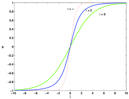
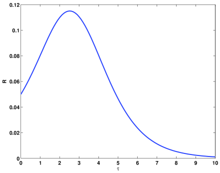
Figure 4: Top: The exact solution (5.16)–(5.17) for different values of $\tau$ and in the limit $\tau\to\infty$. Middle: Enstrophy $E$ versus time $\tau$. The dotted curve shows the value of $E$ at the viscous shock $w_{\infty}(\xi)=\tanh(\xi)$. Bottom: Enstrophy’s rate of change $R$ versus time $\tau$.

Corollary 2

Fix $\delta>0$. There exist $K>0$ and $C>0$ such that for all $k\geq K$, we have

$$\sup_{x\in\mathbb{R}}\left|u(x,t)-u_{\infty}(x)\right|\leq\frac{C}{k^{\delta}},\quad\mbox{\rm for all}\;\;t\geq T_{*}:=\frac{(1+\delta)\log(k)}{12k^{2}}.$$ (5.18)

Proof.

Bound (5.18) follows from (5.12) with $m=0$ after the transformation (5.9). ∎

Remark 6

We actually have shown convergence of $u$ to $u_{\infty}$ in $H^{s}$ norm for any $s\geq 0$, which follows from the exponential decay in $\xi$ and $\tau$.

Figure 4 shows the exact solution $w(\xi,\tau)$ for different values of $\tau$ together with the rescaled enstrophy $E=\int_{0}^{\infty}w_{\xi}^{2}d\xi$ and its rate of change $R=2\int_{0}^{\infty}(w_{\xi}^{3}-w_{\xi\xi}^{2})d\xi$ versus $\tau$. The relevant integrals are approximated by using the MATLAB quad function. The enstrophy $E$ is a monotonically increasing function to the value $E_{\infty}=\frac{2}{3}$, whereas the rate of change $R$ is initially increasing and then decreasing to $R_{\infty}=0$. Note that by Lemma 5.12, we have exponentially rapid convergence $\|w(\cdot,\tau)-w_{\infty}\|_{H^{1}}\to 0$ as $\tau\to\infty$.

If ${\cal E}=E(u_{0})=\frac{32}{3}k^{3}$, then bound (5.18) shows that

$$E(u_{\infty})=\mathcal{O}(\mathcal{E})\quad\mbox{\rm and}\quad T_{*}=\mathcal{O}(\mathcal{E}^{-2/3}\log(\mathcal{E}))\quad\mbox{\rm as}\quad\mathcal{E}\to\infty.$$ (5.19)

The asymptotic result (5.19) is included in the scaling law (2.17) of Theorem 2. We have not achieved the maximal increase of the enstrophy with the initial data (5.11) given by the instantaneous maximizer of Lemma 5.7. To achieve the maximal growth of the enstrophy, we shall modify the initial data $u_{0}$.

5.2 Initial condition with arbitrary $l$

Let us consider a more general initial condition,

$$u_{0}(x)=-4k\tanh(lx),\quad\Rightarrow\quad w_{0}(\xi)=\tanh(\xi/a),$$ (5.20)

where $a=\frac{4k}{l}$ is the only parameter of the initial-value problem (5.10) with initial data (5.20). For analysis needed in the proof of Theorem 2, we need convergence of the solution $w(\xi,\tau)$ to the viscous shock $w_{\infty}(\xi)=\tanh(\xi)$ in the $H^{1}$-norm as the time $\tau$ gets large, and the smallness of $w(\xi,\tau)-w_{\infty}(\xi)$ at large values of $\xi$ for all times $\tau\geq 0$. Both objectives are achieved in the following result.

Lemma 6

Fix $\delta>0$. There are constants $A>0$ and $C>0$ such that for all $a\geq A$, a unique solution of the initial-value problem (5.10) with initial data (5.20) satisfies

$$\sup_{\xi\in\mathbb{R}}\left|w(\xi,\tau)-\tanh(\xi)\right|\leq\frac{C}{a^{3\delta+\delta^{2}}\tau^{1/2}}\quad\mbox{\rm for all}\quad\tau\geq\frac{1}{2}(1+\delta)^{2}a\log(a)$$ (5.21)

Furthermore, for any integer $m\geq 0$, there are constants $A_{m}>0$ and $C_{m}>0$, such that for all $a\geq A_{m}$, we have

$$\left|\partial_{\xi}^{m}\left(w(\xi,\tau)-\tanh(\xi)\right)\right|\leq\frac{C_{m}}{a^{1+m+\delta}}\quad\mbox{\rm for all}\quad|\xi|\geq\frac{1}{2}(1+\delta)^{2}a\log(a)\quad\mbox{\rm and}\quad\tau\geq 0.$$ (5.22)

Proof.

Using the Cole–Hopf transformation (5.13), we rewrite the initial-value problem (5.10) with initial data (5.20) in the form,

$$\left\{\begin{array}[]{l}\psi_{\tau}=\psi_{\xi\xi},\quad\quad\quad\quad\quad\;\;\xi\in\mathbb{R},\quad\tau\in\mathbb{R}_{+},\\ \psi|_{\tau=0}=\cosh^{a}(\xi/a),\quad\xi\in\mathbb{R}.\end{array}\right.$$ (5.23)

The initial data can be represented in the form,

$$\psi|_{\tau=0}=\frac{1}{2^{a}}e^{|\xi|}\phi_{a}(\xi),\quad\phi_{a}(\xi)=(1+e^{-2|\xi|/a})^{a}.$$

The function $\phi_{a}$ is bounded by its value at $\xi=0$,

$$1\leq\phi_{a}(\xi)\leq 2^{a},\quad\xi\in\mathbb{R},$$ (5.24)

but the upper bound diverges quickly as $a\to\infty$. On the other hand, for large values of $\xi$, the function $\phi_{a}$ decays to $1$ exponentially rapidly.

Fix $\delta>0$ and define $\xi_{a}:=\frac{1+\delta}{2}a\log(a)$. For sufficiently large $a\gg 1$, there is $C>0$ such that

$$0\leq\phi_{a}(\xi)-1=e^{a\log(1+e^{-2|\xi|/a})}-1\leq Cae^{-2|\xi|/a}\leq\frac{C}{a^{\delta}},\quad|\xi|\geq\xi_{a}.$$ (5.25)

The upper bound in (5.25) converges to zero as $a\to\infty$.

To bound derivatives of $\phi_{a}$ in $\xi$, we note that

$$\phi_{a}^{\prime}(\xi)=-2(1+e^{-2\xi/a})^{a-1}e^{-2\xi/a},\quad\xi>0,$$ (5.26)

which implies that

$$\sup_{\xi\in\mathbb{R}_{+}}|\phi_{a}^{\prime}(\xi)|=2^{a},\quad\sup_{\xi\geq\xi_{a}}|\phi_{a}^{\prime}(\xi)|\leq\frac{C}{a^{1+\delta}}.$$ (5.27)

Writing (5.26) as

$$\frac{d}{d\xi}\log\phi_{a}(\xi)=-\frac{2e^{-2\xi/a}}{1+e^{-2\xi/a}},\quad\Rightarrow\quad\frac{d^{2}}{d\xi^{2}}\log\phi_{a}(\xi)=\frac{1}{a}{\rm sech}^{2}\left(\frac{\xi}{a}\right),\quad\xi>0,$$

and using (5.24) and (5.25), we obtain by induction that, for any integer $m\geq 0$, there is $C_{m}>0$ such that

$$\sup_{\xi\in\mathbb{R}_{+}}|\partial_{\xi}^{m}\phi_{a}(\xi)|\leq C_{m}2^{a},\quad\sup_{\xi\geq\xi_{a}}|\partial_{\xi}^{m}\phi_{a}(\xi)|\leq\frac{C_{m}}{a^{m+\delta}}.$$ (5.28)

The solution of the initial-value problem for the heat equation (5.23) is obtained explicitly as

$$\psi(\xi,\tau) = \frac{1}{2^{a}\sqrt{4\pi\tau}}\int_{-\infty}^{\infty}e^{-\frac{(\xi-\eta)^{2}}{4\tau}+|\eta|}\phi_{a}(\eta)d\eta$$

$$= \frac{1}{2^{a}\sqrt{\pi}}e^{\tau}\left(e^{\xi}\int_{-z_{+}}^{\infty}e^{-z^{2}}\phi_{a}(\xi+2\tau+2\sqrt{\tau}z)dz+e^{-\xi}\int_{-\infty}^{z_{-}}e^{-z^{2}}\phi_{a}(\xi-2\tau+2\sqrt{\tau}z)dz\right),$$

where

$$z_{\pm}=\frac{2\tau\pm\xi}{2\sqrt{\tau}}.$$

We shall rewrite the solution in the equivalent form,

$$\psi(\xi,\tau)=\frac{1}{2^{a-1}}e^{\tau}\cosh(\xi)\left[1+\Psi(\xi,\tau)\right],\quad\Psi(\xi,\tau):=\frac{e^{\xi}\psi_{+}(\xi,\tau)+e^{-\xi}\psi_{-}(\xi,\tau)}{\sqrt{\pi}(e^{\xi}+e^{-\xi})},$$ (5.29)

where

$$\psi_{+}(\xi,\tau) := \int_{-z_{+}}^{\infty}e^{-z^{2}}\phi_{a}(\xi+2\tau+2\sqrt{\tau}z)dz-\sqrt{\pi},$$ (5.30)

$$\psi_{-}(\xi,\tau) := \int_{-\infty}^{z_{-}}e^{-z^{2}}\phi_{a}(\xi-2\tau+2\sqrt{\tau}z)dz-\sqrt{\pi}.$$ (5.31)

Using the Cole–Hopf transformation (5.13) and the explicit representation (5.29), we write the solution of the Burgers equation (5.10) in the form,

$$w(\xi,\tau)=\tanh(\xi)+\tilde{w}(\xi,\tau),\quad\tilde{w}(\xi,\tau)=\frac{\partial_{\xi}\Psi(\xi,\tau)}{1+\Psi(\xi,\tau)},$$ (5.32)

where

$$\partial_{\xi}\Psi(\xi,\tau)=\frac{e^{\xi}\partial_{\xi}\psi_{+}(\xi,\tau)+e^{-\xi}\partial_{\xi}\psi_{-}(\xi,\tau)}{\sqrt{\pi}(e^{\xi}+e^{-\xi})}+\frac{1}{2\sqrt{\pi}}{\rm sech}^{2}(\xi)(\psi_{+}(\xi,\tau)-\psi_{-}(\xi,\tau)).$$

We first prove bound (5.21). Because $\psi$ is even in $\xi$, we can consider $\xi\geq 0$ without the loss of generality. To analyze $\psi_{+}$, we define

$$z_{a}:=z_{+}-\frac{\xi_{a}}{2\sqrt{\tau}}=\frac{\xi-\xi_{a}+2\tau}{2\sqrt{\tau}},$$

so that $z\geq-z_{a}$ corresponds to $\xi\geq\xi_{a}$ in the argument of $\phi_{a}(\xi)$. For any $\xi\geq 0$ and $\tau\geq\tau_{a}:=(1+\delta)\xi_{a}$, we have

$$z_{a}\geq\frac{2\tau_{a}-\xi_{a}}{2\sqrt{\tau_{a}}}\geq\frac{1+2\delta}{2\sqrt{2}}\sqrt{a\log(a)},$$

which shows that $z_{a}\to\infty$ as $a\to\infty$. The term $\psi_{+}(\xi,\tau)$ can be split into the sum of three terms

$$\psi_{+}(\xi,\tau) = \left(\int_{-z_{a}}^{\infty}e^{-z^{2}}dz-\sqrt{\pi}\right)+\int_{-z_{a}}^{\infty}e^{-z^{2}}(\phi_{a}(\xi+2\tau+2\sqrt{\tau}z)-1)dz$$ (5.33)

$$\quad+\int_{-z_{+}}^{-z_{a}}e^{-z^{2}}\phi_{a}(\xi+2\tau+2\sqrt{\tau}z)dz\equiv I+II+III.$$

For all $\xi\geq 0$ and $\tau\geq\tau_{a}$, we obtain

$$I=\int_{-\infty}^{-z_{a}}e^{-z^{2}}dz\leq\frac{1}{2z_{a}}e^{-z_{a}^{2}}\leq\frac{\sqrt{2}}{(1+2\delta)\sqrt{a\log(a)}}e^{-\frac{(1+2\delta)^{2}}{8}a\log(a)}$$

and

$$III\leq 2^{a}\int_{-z_{+}}^{-z_{a}}e^{-z^{2}}dz\leq\frac{2^{a}}{2z_{a}}e^{-z_{a}^{2}}\leq\frac{\sqrt{2}}{(1+2\delta)\sqrt{a\log(a)}}e^{-\frac{(1+2\delta)^{2}}{8}a\log(a)+a\log(2)},$$

where the upper bounds are exponentially small as $a\to\infty$ and the bound (5.24) has been used. Using bound (5.25), we obtain

$$II\leq Ca\int_{-z_{a}}^{\infty}e^{-z^{2}-2(\xi+2\tau+2\sqrt{\tau}z)/a}dz\leq\sqrt{\pi}Cae^{-2(1+\delta)^{2}\log(a)}\leq\frac{C}{a^{1+4\delta+2\delta^{2}}}.$$

Combining these terms and dropping the exponentially small terms, we infer that for any fixed $\delta>0$ and for sufficiently large $a\gg 1$, there is $C>0$ such that

$$\sup_{\tau\geq\tau_{a}}\sup_{\xi\geq 0}|\psi_{+}(\xi,\tau)|\leq\frac{C}{a^{1+4\delta+2\delta^{2}}}.$$ (5.34)

To analyze $\psi_{-}$, we define

$$\hat{z}_{a}:=z_{-}-\frac{\xi_{a}}{2\sqrt{\tau}}=\frac{-\xi-\xi_{a}+2\tau}{2\sqrt{\tau}},$$

so that $z\leq z_{a}$ corresponds to $\xi\leq-\xi_{a}$ in the argument of $\phi_{a}(\xi)$. For any $0\leq\xi\leq\xi_{a}$ and $\tau\geq\tau_{a}$, we have

$$\hat{z}_{a}\geq\frac{\tau_{a}-\xi_{a}}{\sqrt{\tau_{a}}}\geq\frac{\delta}{\sqrt{2}}\sqrt{a\log(a)},$$

which shows that $\hat{z}_{a}\to\infty$ as $a\to\infty$. The term $\psi_{-}(\xi,\tau)$ can be split into the sum of three terms

$$\psi_{-}(\xi,\tau) = \left(\int_{-\infty}^{\hat{z}_{a}}e^{-z^{2}}dz-\sqrt{\pi}\right)+\int_{-\infty}^{\hat{z}_{a}}e^{-z^{2}}(\phi_{a}(\xi-2\tau+2\sqrt{\tau}z)-1)dz$$ (5.35)

$$+\int_{\hat{z}_{a}}^{z_{-}}e^{-z^{2}}\phi_{a}(\xi-2\tau+2\sqrt{\tau}z)dz\equiv I+II+III.$$

Using computations similar to those for $\psi_{+}(\xi,\tau)$, we obtain for any $0\leq\xi\leq\xi_{a}$ and $\tau\geq\tau_{a}$,

$$I\leq\frac{1}{\delta\sqrt{2a\log(a)}}e^{-\frac{\delta^{2}}{2}a\log(a)},\quad II\leq\frac{C}{a^{3\delta+2\delta^{2}}},\quad III\leq\frac{1}{\delta\sqrt{2a\log(a)}}e^{-\frac{\delta^{2}}{2}a\log(a)+a\log(2)}.$$

Again, for any fixed $\delta>0$ and for sufficiently large $a\gg 1$, there is $C>0$ such that

$$\sup_{\tau\geq\tau_{a}}\sup_{0\leq\xi\leq\xi_{a}}|\psi_{-}(\xi,\tau)|\leq\frac{C}{a^{3\delta+2\delta^{2}}}.$$ (5.36)

Finally, the exponential factor in front of $\psi_{-}$ yields the following simple estimate:

$$\sup_{\xi\geq\xi_{a}}e^{-2\xi}\psi_{-}(\xi,\tau)\leq\sqrt{\pi}(2^{a}-1)e^{-2\xi_{a}}\leq Ce^{-(1+\delta)a\log(a)+a\log(2)},\quad\tau\geq 0,$$ (5.37)

where the upper bound is exponentially small as $a\to\infty$.

Because of the symmetry for $\xi\leq 0$, we infer from (5.34), (5.36), and (5.37) that for any fixed $\delta>0$ and for sufficiently large $a\gg 1$, there is constant $C>0$ such that

$$\sup_{\tau\geq\tau_{a}}\sup_{\xi\in\mathbb{R}}|\Psi(\xi,\tau)|\leq\frac{C}{a^{3\delta+2\delta^{2}}}.$$ (5.38)

This result shows that $\Psi$ is small for $\tau\geq\tau_{a}$ in the denominator of the exact solution (5.32).

We now proceed with similar expressions for $\partial_{\xi}\psi_{+}(\xi,\tau)$ and $\partial_{\xi}\psi_{-}(\xi,\tau)$. Using the representation (5.33), we find

$$\partial_{\xi}I=\frac{1}{2\sqrt{\tau}}e^{-z_{a}^{2}},$$ (5.39)

$$\partial_{\xi}II = \frac{1}{2\sqrt{\tau}}e^{-z_{a}^{2}}(\phi_{a}(\xi_{a})-1)+\frac{1}{2\sqrt{\tau}}\int_{-z_{a}}^{\infty}e^{-z^{2}}\partial_{z}\phi_{a}(\xi+2\tau+2\sqrt{\tau}z)dz$$ (5.40)

$$= \frac{1}{\sqrt{\tau}}\int_{-z_{a}}^{\infty}ze^{-z^{2}}\left(\phi_{a}(\xi+2\tau+2\sqrt{\tau}z)-1\right)dz,$$

and

$$\partial_{\xi}III = \frac{1}{2\sqrt{\tau}}\left[e^{-z_{+}^{2}}\phi_{a}(0)-e^{-z_{a}^{2}}\phi_{a}(\xi_{a})\right]+\frac{1}{2\sqrt{\tau}}\int_{-z_{+}}^{-z_{a}}e^{-z^{2}}\partial_{z}\phi_{a}(\xi+2\tau+2\sqrt{\tau}z)dz$$ (5.41)

$$= \frac{1}{\sqrt{\tau}}\int_{-z_{+}}^{-z_{a}}ze^{-z^{2}}\phi_{a}(\xi+2\tau+2\sqrt{\tau}z)dz.$$

Using bounds (5.24) and (5.25), we obtain that for any $\xi\geq 0$ and $\tau\geq\tau_{a}$ there is $C>0$ such that

$$\partial_{\xi}I\leq\frac{C}{\sqrt{\tau}}e^{-\frac{(1+2\delta)^{2}}{8}a\log(a)},\quad|\partial_{\xi}II|\leq\frac{C}{\sqrt{\tau}a^{1+4\delta+2\delta^{2}}},\quad|\partial_{\xi}III|\leq\frac{C}{\sqrt{\tau}}e^{-\frac{(1+2\delta)^{2}}{8}a\log(a)+a\log(2)},$$

where in the computations for $\partial_{\xi}II$ we have used the fact that the function $\sqrt{\tau}e^{-4\tau/a}$ is monotonically decreasing for any $\tau>\frac{a}{8}$, whereas $\tau_{a}\gg\mathcal{O}(a)$ as $a\to\infty$.

Combining all bounds and dropping the exponentially small factors, we infer that for any fixed $\delta>0$ and sufficiently large $a\gg 1$, there is $C>0$ such that

$$\sup_{\xi\geq 0}|\partial_{\xi}\psi_{+}(\xi,\tau)|\leq\frac{C}{\sqrt{\tau}a^{1+4\delta+2\delta^{2}}},\quad\tau\geq\tau_{a}.$$ (5.42)

Similarly, we obtain

$$\sup_{0\leq\xi\leq\xi_{a}}|\partial_{\xi}\psi_{-}(\xi,\tau)|\leq\frac{C}{\sqrt{\tau}a^{3\delta+2\delta^{2}}},\quad\tau\geq\tau_{a}$$ (5.43)

and

$$|\partial_{\xi}\psi_{-}(\xi,\tau)|\leq\frac{2^{a}}{\sqrt{\tau}}\int_{-\infty}^{\sqrt{\tau}-\xi/(2\sqrt{\tau})}|z|e^{-z^{2}}dz,\quad\tau\geq 0,\quad\xi\geq\xi_{a},$$ (5.44)

which yields

$$\sup_{\xi\geq\xi_{a}}e^{-2\xi}|\partial_{\xi}\psi_{-}(\xi,\tau)|\leq\frac{C2^{a}}{\sqrt{\tau}}e^{-2\xi_{a}}\leq\frac{C}{\sqrt{\tau}}e^{-(1+\delta)a\log(a)+a\log(2)},\quad\tau\geq\tau_{a}.$$ (5.45)

Because of the symmetry for $\xi\leq 0$, we infer from (5.42), (5.43), and (5.45) that for any fixed $\delta>0$ and for sufficiently large $a\gg 1$, there is constant $C>0$ such that

$$\sup_{\xi\in\mathbb{R}}\left|\frac{e^{\xi}\partial_{\xi}\psi_{+}(\xi,\tau)+e^{-\xi}\partial_{\xi}\psi_{-}(\xi,\tau)}{e^{\xi}+e^{-\xi}}\right|\leq\frac{C}{\sqrt{\tau}a^{3\delta+2\delta^{2}}},\quad\tau\geq\tau_{a}.$$ (5.46)

We now need to estimate the difference $\psi_{+}(\xi,\tau)-\psi_{-}(\xi,\tau)$. We can write

$$\psi_{+}(\xi,\tau)-\psi_{-}(\xi,\tau) = \frac{1}{2\sqrt{\tau}}\int_{0}^{\infty}\phi_{a}(\eta)\left[e^{-\frac{(\eta-\xi-2\tau)^{2}}{4\tau}}-e^{-\frac{(\eta+\xi-2\tau)^{2}}{4\tau}}\right]d\eta$$

$$= \frac{1}{\sqrt{\tau}}\left(\int_{-2\tau}^{-\tau}+\int_{-\tau}^{\infty}\right)\phi_{a}(\eta+2\tau)e^{-\frac{\xi^{2}+\eta^{2}}{4\tau}}\sinh\left(\frac{\xi\eta}{2\tau}\right)d\eta\equiv I+II.$$

For any $|\xi|\leq\frac{1}{2}\tau$, we have

$$|I| = \frac{1}{\sqrt{\tau}}\int_{\tau}^{2\tau}\phi_{a}(2\tau-\eta)e^{-\frac{\xi^{2}+\eta^{2}}{4\tau}}\sinh\left(\frac{|\xi|\eta}{2\tau}\right)d\eta$$

$$\leq \frac{2^{a}}{\sqrt{\tau}}\int_{\tau}^{\infty}e^{-\frac{(\eta-|\xi|)^{2}}{4\tau}}d\eta\leq\frac{2^{a}\sqrt{\tau}}{\tau-|\xi|}e^{-\frac{(\tau-|\xi|)^{2}}{4\tau}}\leq\frac{2^{a+1}}{\sqrt{\tau}}e^{-\frac{1}{16}\tau}.$$

Then, we represent

$$II = \frac{1}{\sqrt{\tau}}\int_{-\tau}^{\infty}(\phi_{a}(\eta+2\tau)-1)e^{-\frac{\xi^{2}+\eta^{2}}{4\tau}}\sinh\left(\frac{\xi\eta}{2\tau}\right)d\eta+\frac{1}{\sqrt{\tau}}\int_{-\tau}^{\infty}e^{-\frac{\xi^{2}+\eta^{2}}{4\tau}}\sinh\left(\frac{\xi\eta}{2\tau}\right)d\eta$$

$$\equiv II_{a}+II_{b},$$

and estimate

$$|II_{b}|=\frac{1}{\sqrt{\tau}}\int_{\tau}^{\infty}e^{-\frac{\xi^{2}+\eta^{2}}{4\tau}}\sinh\left(\frac{|\xi|\eta}{2\tau}\right)d\eta\leq\frac{1}{\sqrt{\tau}}\int_{\tau}^{\infty}e^{-\frac{(\eta-|\xi|)^{2}}{4\tau}}d\eta\leq\frac{2}{\sqrt{\tau}}e^{-\frac{1}{16}\tau}.$$

and

$$|II_{a}|\leq\frac{Ca}{\sqrt{\tau}}e^{2|\xi|/a-4\tau/a}\int_{-\tau}^{\infty}e^{-\frac{(\eta-|\xi|+4\tau/a)^{2}}{4\tau}}d\eta\leq\frac{Ca}{\sqrt{\tau}}\sqrt{\tau}e^{-3\tau/a}\leq\frac{C\sqrt{\log(a)}}{\sqrt{\tau}a^{3\delta+3\delta^{2}/2}},$$

where we have used again the fact that the function $\sqrt{\tau}e^{-3\tau/a}$ is monotonically decreasing for any $\tau>\frac{a}{6}$, whereas $\tau_{a}\gg\mathcal{O}(a)$ as $a\to\infty$. Because $I$ and $II_{b}$ are exponentially small in $a$ for all $\tau\geq\tau_{a}$, there is $C>0$ such that

$$\sup_{|\xi|\leq\frac{1}{2}\tau}|\psi_{+}(\xi,\tau)-\psi_{-}(\xi,\tau)|\leq\frac{C\sqrt{\log(a)}}{\sqrt{\tau}a^{3\delta+3\delta^{2}/2}}\leq\frac{C}{\sqrt{\tau}a^{3\delta+\delta^{2}}},\quad\tau\geq\tau_{a}.$$ (5.47)

On the other hand, for any $|\xi|\geq\frac{1}{2}\tau$, there is $C>0$ such that

$${\rm sech}^{2}(\xi)|\psi_{+}(\xi,\tau)-\psi_{-}(\xi,\tau)|\leq C2^{a}e^{-\tau},$$ (5.48)

which is exponentially small in $a$ for all $\tau\geq\tau_{a}$. It follows from (5.47)–(5.48) that for any fixed $\delta>0$ and for sufficiently large $a\gg 1$, there is constant $C>0$ such that

$$\sup_{\xi\in\mathbb{R}}{\rm sech}^{2}(\xi)|\psi_{+}(\xi,\tau)-\psi_{-}(\xi,\tau)|\leq\frac{C}{\sqrt{\tau}a^{3\delta+\delta^{2}}},\quad\tau\geq\tau_{a}.$$ (5.49)

Representation (5.32) and bounds (5.38), (5.46) and (5.49) yield the desired bound (5.21).

We can now prove bound (5.22) for $m=0$. Using the exponential factors, we have bound (5.37), which is exponentially small as $a\to\infty$ for all $\xi\geq\xi_{a}$ and $\tau\geq 0$. We can rewrite bounds (5.44) and (5.48) in the equivalent form:

$$e^{-2\xi}|\partial_{\xi}\psi_{-}(\xi,\tau)|\leq C2^{a}e^{-2\xi_{a}},\quad\xi\geq\xi_{a},\quad\tau\geq 0,$$

and

$${\rm sech}^{2}(\xi)|\psi_{+}(\xi,\tau)-\psi_{-}(\xi,\tau)|\leq C2^{a}e^{-2\xi_{a}},\quad\xi\geq\xi_{a},\quad\tau\geq 0.$$

Therefore, these bounds are also exponentially small as $a\to\infty$ and we only need to show that the terms $\psi_{+}(\xi,\tau)$ and $\partial_{\xi}\psi_{+}(\xi,\tau)$ remain small for all $\xi\geq(1+\delta)\xi_{a}$ and $\tau\geq 0$. We need the extra factor $(1+\delta)$ in $\xi\geq(1+\delta)\xi_{a}$ to ensure that $z_{a}$ is bounded from below by

$$z_{a}=\frac{\xi-\xi_{a}+2\tau}{2\sqrt{\tau}}\geq\frac{\delta\xi_{a}+2\tau}{2\sqrt{\tau}}\geq\sqrt{2\delta\xi_{a}}=\sqrt{\delta(1+\delta)a\log(a)},$$

where we have used the fact that the function $\sqrt{\tau}+\frac{\delta\xi_{a}}{2\sqrt{\tau}}$ reaches minimum at $\tau_{0}=\frac{\delta\xi_{a}}{2}>0$.

Using the splitting of $\psi_{+}$ in (5.33), we infer that the estimates for $I$ and $III$ produce exponentially small terms in $a$, whereas the estimate for $II$ produces an algebraically small term in $a$. As a result of analysis similar to the one for (5.34), we find that there is $C>0$ such that

$$\sup_{\tau\geq 0}\sup_{\xi\geq(1+\delta)\xi_{a}}|\psi_{+}(\xi,\tau)|\leq Cae^{-2(1+\delta)\xi_{a}/a}\leq\frac{C}{a^{2\delta+\delta^{2}}}.$$ (5.50)

Using the exact expression (5.39) and the fact that the function $\frac{1}{\sqrt{\tau}}e^{-(\delta\xi_{a}+2\tau)^{2}/(4\tau)}$ reaches maximum for $\tau\geq 0$ at

$$\tau_{0}=\frac{1}{4}\left(\sqrt{1+4\delta^{2}\xi_{a}^{2}}-1\right)\approx\frac{\delta\xi_{a}}{2},$$

we obtain

$$\partial_{\xi}I\leq\frac{C}{\sqrt{a\log(a)}}e^{-\delta(1+\delta)a\log(a)}.$$

Similarly, using the exact expression (5.41), we obtain

$$\left|\partial_{\xi}III\right|\leq\frac{C}{\sqrt{a\log(a)}}e^{-\delta(1+\delta)a\log(a)+a\log(2)}.$$

Using the exact expression (5.40) rewritten as

$$\partial_{\xi}II=\frac{1}{2\sqrt{\tau}}e^{-z_{a}^{2}}(\phi_{a}(\xi_{a})-1)+\int_{-z_{a}}^{\infty}e^{-z^{2}}\phi_{a}^{\prime}(\xi+2\tau+2\sqrt{\tau}z)dz,$$

and the bounds (5.25) and (5.27), we obtain

$$\left|\partial_{\xi}II\right|\leq\frac{C}{\sqrt{\log(a)}a^{\delta+1/2}}e^{-\delta(1+\delta)a\log(a)}+\frac{C}{a^{1+\delta}}.$$

Combining these estimates together, we infer that there is $C>0$ such that

$$\sup_{\tau\geq 0}\sup_{\xi\geq(1+\delta)\xi_{a}}|\partial_{\xi}\psi_{+}(\xi,\tau)|\leq\frac{C}{a^{1+\delta}}.$$ (5.51)

Using (5.50) and (5.51), we obtain the desired bound (5.22) for $m=0$. Bound (5.22) for $m\in\mathbb{N}$ follows by recursion from the higher-order derivatives of the exact solution (5.32), the decompositions (5.33) and (5.35), and the bound (5.28) on the higher-order derivatives of the function $\phi_{a}$. ∎

Corollary 3

Fix $\delta>0$ and let $a=\frac{4k}{l}$. There exist $A>0$ and $C>0$ such that for all $a\geq A$,

$$\sup_{x\in\mathbb{R}}\left|u(x,t)-u_{\infty}(x)\right|\leq\frac{C}{a^{3\delta+\delta^{2}}t^{1/2}},\quad\mbox{\rm for all}\;\;t\geq T_{*}:=\frac{(1+\delta)^{2}a\log(a)}{32k^{2}}.$$ (5.52)

Proof.

Bound (5.52) follows from (5.21) after the scaling transformation (5.9). ∎

Remark 7

We can also prove convergence of $u$ to $u_{\infty}$ in $H^{1}$ norm but it requires some decay as $|\xi|\to\infty$ and an extension of bound (5.21) for the first derivative in $\xi$, which we do not establish in Lemma 5.12. Note that bounds (5.21) and (5.22) will be applied on large but finite intervals in $\xi$.

Figure 5 shows the exact solution $w(\xi,\tau)$ with $a=10$ for different values of $\tau$ together with the rescaled enstrophy $E=\int_{0}^{\infty}w_{\xi}^{2}d\xi$. The integrals in the exact solution (5.32) were approximated by using the MATLAB quad function. The behavior of $w$ and $E$ looks similar to the case $a=4$ shown on Figure 4 but it takes longer for $E$ to approach to the limit $E_{\infty}=\frac{2}{3}$ from the initially smaller value $E_{0}=\frac{2}{3a}$.

Explicit computation with the initial data (5.20) yields $E(u_{0})=\frac{32}{3}k^{2}l$, whereas we recall that $E(u_{\infty})=\frac{128}{3}k^{3}$. If $l=\mathcal{O}(1)$ as $k\to\infty$, we have $k=\mathcal{O}(\mathcal{E}^{1/2})$ and hence

$$E(u_{\infty})=\mathcal{O}(\mathcal{E}^{3/2}),\quad T_{*}=\mathcal{O}({\cal E}^{-1/2}\log({\cal E})),\quad\mbox{\rm as}\quad\mathcal{E}\to\infty.$$ (5.53)

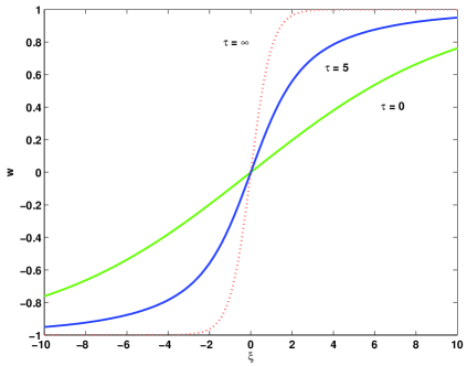
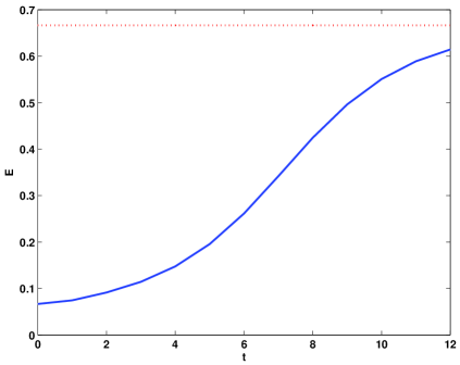
Figure 5: Left: The exact solution (5.32) with $a=10$ for different values of $\tau$ and in the limit $\tau\to\infty$. Right: Enstrophy $E$ versus time $\tau$. The dotted curve shows the value of $E$ at the viscous shock $w_{\infty}(\xi)=\tanh(\xi)$.

If $l=(1+\Delta)\log(k)$, then Lemma 2.13 implies that $k=\mathcal{O}(\mathcal{E}^{1/2}\log^{-1/2}(\mathcal{E}))$. From (5.52), we have

$$T_{*}=\frac{(1+\delta)^{2}}{8(1+\Delta)k}\left[1+\mathcal{O}\left(\frac{\log\log(k)}{\log(k)}\right)\right].$$ (5.54)

Hence we have

$$E(u_{\infty})=\mathcal{O}(\mathcal{E}^{3/2}\log^{-3/2}(\mathcal{E}))\quad\mbox{\rm and}\quad T_{*}=\mathcal{O}({\cal E}^{-1/2}\log^{1/2}({\cal E}))\quad\mbox{\rm as}\quad\mathcal{E}\to\infty.$$ (5.55)

The asymptotic result (5.55) is included in the scaling law (2.18) of Theorem 2. On the other hand, the maximal rate (5.53) can not be achieved, because if $l=\mathcal{O}(1)$, then $a=\mathcal{O}(k)$ and the lower bound on the time $\tau\geq\frac{1}{2}(1+\delta)^{2}a\log(a)$ in bound (5.21) is beyond the time interval $\tau\in(0,k)$ in Lemma 3 as $k\to\infty$.

6 Dynamics of a viscous shock in a bounded domain

By Lemma 3, the initial-value problem (1.1) is replaced by the equivalent problem,

$$\left\{\begin{array}[]{l}w_{\tau}=2ww_{\xi}+w_{\xi\xi},\quad\quad|\xi|<2(k-\tau),\quad\tau\in(0,k),\\ w|_{\tau=0}=w_{0},\quad\quad\quad\quad\;\;|\xi|\leq 2k,\end{array}\right.$$ (6.1)

subject to the initial condition $w_{0}(\xi)=f(\xi/4k)$ and the inhomogeneous boundary conditions $w=\pm 1$ at $\xi=\pm 2(k-\tau)$, where $f$ is given by either (2.8) or (2.9).

Let us define the norm

$$\|w\|_{L^{2}_{k,\tau}}:=\left(\int_{-2(k-\tau)}^{2(k-\tau)}|w(\xi,\tau)|^{2}d\xi\right)^{1/2}.$$ (6.2)

An approximate solution of the initial-value problem (6.1) can be thought in the form,

$$w_{\rm app}(\xi,\tau)=\frac{\partial}{\partial\xi}\log\psi_{\rm app}(\xi,\tau),$$ (6.3)

where $\psi_{\rm app}$ is a solution of the homogeneous heat equation on the real line. For $f$ in either (2.8) or (2.9), the solution is constructed in Lemmas 5.12 or 6, respectively. We shall assume that

$$0\leq\frac{\partial}{\partial\xi}w_{\rm app}(\xi,\tau)\leq 1,\quad\xi\in\mathbb{R},\quad\tau\in\mathbb{R}_{+},$$ (6.4)

which is a reasonable assumption for a monotonic transition from $w_{\rm app,0}(\xi)=\tanh(\xi/a)$ with either $a=4$ or $a\to\infty$ as $k\to\infty$ to the viscous shock $w_{\infty}(\xi)=\tanh(\xi)$.

We write $w_{\rm app}(\xi,\tau)=\tanh(\xi)+\tilde{w}(\xi,\tau)$ and assume that for any fixed $C_{0}\in(0,1)$, and for sufficiently large $k\gg 1$, there is a small $C_{k}>0$ such that

$$\sup_{\tau\in[0,C_{0}k]}\left(|\tilde{w}(2(k-\tau),\tau)|+\left|\frac{d}{d\tau}\tilde{w}(2(k-\tau),\tau)\right|+\left|\frac{d^{2}}{d\tau^{2}}\tilde{w}(2(k-\tau),\tau)\right|\right)\leq\frac{C_{k}}{k},$$ (6.5)

where $C_{k}\to 0$ as $k\to\infty$.

Furthermore, we assume that for sufficiently large $k\gg 1$, there is a small $D_{k}>0$ such that

$$\sup_{\xi\in[-2k,2k]}\left(\left|w_{0}(\xi)-w_{{\rm app},0}(\xi)\right|+\left|w_{0}^{\prime}(\xi)-w_{{\rm app},0}^{\prime}(\xi)\right|\right)\leq\frac{D_{k}}{k^{3/2}},$$ (6.6)

where $D_{k}\to 0$ as $k\to\infty$.

Using the Cole–Hopf transformation, we rewrite the initial-value problem (6.1) in the form,

$$w=\frac{\psi_{\xi}}{\psi}\quad\Rightarrow\quad\left\{\begin{array}[]{l}\psi_{\tau}=\psi_{\xi\xi},\quad\quad\;\;|\xi|<2(k-\tau),\quad\tau\in(0,k),\\ \psi|_{\tau=0}=\psi_{0},\quad\;\;|\xi|\leq 2k,\end{array}\right.$$ (6.7)

subject to the initial condition $\psi_{0}=\exp\left(\int_{0}^{\xi}w_{0}(\xi^{\prime})d\xi^{\prime}\right)$ and the Robin boundary conditions $\psi_{\xi}=\pm\psi$ at $\xi=\pm 2(k-\tau)$. Using the decomposition

$$\psi=\psi_{\rm app}(1+\Psi),$$ (6.8)

we find the equivalent initial-value problem,

$$\left\{\begin{array}[]{l}\Psi_{\tau}=\Psi_{\xi\xi}+2w_{\rm app}\Psi_{\xi},\quad\quad\quad|\xi|<2(k-\tau),\quad\tau\in(0,k),\\ \Psi|_{\tau=0}=\Psi_{0},\quad\quad\quad\quad\quad\quad\quad|\xi|\leq 2k,\end{array}\right.$$ (6.9)

subject to the initial condition,

$$\Psi_{0}(\xi)=\frac{\psi_{0}(\xi)}{\psi_{{\rm app},0}(\xi)}-1=\exp\left(\int_{0}^{\xi}\left[w_{0}(\xi^{\prime})-w_{{\rm app},0}(\xi^{\prime})\right]d\xi^{\prime}\right)-1,$$ (6.10)

and the Robin inhomogeneous boundary conditions,

$$\Psi_{\xi}=\pm\chi(\tau)(1+\Psi),\quad\xi=\pm 2(k-\tau),\quad\tau\in[0,k],$$ (6.11)

where

$$\chi(\tau)=1-w_{\rm app}(2(k-\tau),\tau)=\frac{2e^{-4(k-\tau)}}{1+e^{-4(k-\tau)}}-\tilde{w}(2(k-\tau),\tau).$$ (6.12)

By bound (6.5) and explicit expression (6.12), for any fixed $C_{0}\in(0,1)$ and for sufficiently large $k\gg 1$, there is a small $C_{k}>0$ such that

$$\sup_{\tau\in[0,C_{0}k]}\left(|\chi(\tau)|+|\chi^{\prime}(\tau)|+|\chi^{\prime\prime}(\tau)|\right)\leq\frac{C_{k}}{k}.$$ (6.13)

Because $C_{k}\to 0$ as $k\to\infty$ in (6.13), the Robin boundary conditions (6.11) converge to the Neumann conditions as $k\to\infty$.

By bound (6.6) and explicit expression (6.10), for sufficiently large $k\gg 1$, there is a small $D_{k}>0$ such that

$$\sup_{\xi\in[-2k,2k]}|\Psi_{0}(\xi)|\leq\frac{D_{k}}{k^{1/2}},\quad\|\Psi_{0}\|_{L^{2}_{k,0}}\leq D_{k},\quad\|\Psi_{0}^{\prime}\|_{L^{2}_{k,0}}+\|\Psi_{0}^{\prime\prime}\|_{L^{2}_{k,0}}\leq\frac{D_{k}}{k}.$$ (6.14)

Because $D_{k}\to 0$ as $k\to\infty$ in (6.14), the initial condition (6.10) converges to $0$ as $k\to\infty$.

Using apriori energy estimates, we prove the following result.

Lemma 7

Assume (6.4), (6.13), and (6.14). Fix $C_{0}\in(0,1)$. There exist constants $K\geq 1$ and $C>0$, such that for all $k\geq K$ and $\tau\in[0,C_{0}k]$, the unique solution of the Burgers equation (6.1) satisfies

$$\|w-w_{\rm app}\|^{2}_{L^{2}_{k,\tau}}+\|\partial_{\xi}(w-w_{\rm app})\|^{2}_{L^{2}_{k,\tau}}\leq C\left(C_{k}+D_{k}^{2}\right)$$ (6.15)

where $C_{k}$ and $D_{k}$ are defined by (6.13) and (6.14).

Proof.

We note the correspondence,

$$w=w_{\rm app}+\frac{\Psi_{\xi}}{1+\Psi}.$$ (6.16)

Fix $C_{0}\in(0,1)$ and introduce the energy for the initial-boundary value problem (6.9),

$$H(\tau):=\frac{1}{2}\|\Psi\|_{L^{2}_{k,\tau}}^{2}+\frac{1}{2}\|\Psi_{\xi}\|_{L^{2}_{k,\tau}}^{2},\quad\tau\in[0,C_{0}k].$$ (6.17)

If $H(\tau)$ is small for all $\tau\in[0,C_{0}k]$, then there is $C>0$ such that

$$\|w-w_{\rm app}\|^{2}_{L^{2}_{k,\tau}}\leq CH(\tau).$$ (6.18)

The initial-boundary value problem (6.9) inherits the local well-posedness of the initial-value problem (1.1) if $\Psi_{0}\in H^{1}([-2k,2k])$ as long as

$$\sup_{|\xi|\leq 2(k-\tau)}|\Psi(\xi,\tau)|<1,\quad\tau\in[0,C_{0}k],$$ (6.19)

to ensure that $1+\Psi(\xi,\tau)>0$ for all $|\xi|\leq 2(k-\tau)$ and $\tau\in[0,k]$. Recalling Sobolev’s embedding of $H^{1}$ to $L^{\infty}$, we have

$$\exists C>0:\quad\sup_{|\xi|\leq 2(k-\tau)}|\Psi(\xi,\tau)|\leq C\sqrt{H(\tau)},\quad\tau\in[0,C_{0}k],$$ (6.20)

hence the constraint (6.19) is satisfied if $H(\tau)$ remains small for all $\tau\in[0,C_{0}k]$.

Computations are simplified for the even solutions $\Psi(-\xi,\tau)=\Psi(\xi,\tau)$, which generate odd solutions $w(-\xi,\tau)=-w(\xi,\tau)$ of the Burgers equation (6.1). Multiplying the heat equation (6.9) by the solution $\Psi$ and integrating in $\xi$ over the time-dependent interval $[-\xi_{+}(\tau),\xi_{+}(\tau)]$ with $\xi_{+}(\tau)=2(k-\tau)$, we obtain

$$\frac{1}{2}\frac{d}{d\tau}\|\Psi\|_{L^{2}_{k,\tau}}^{2}+2\Psi_{+}^{2}(\tau) = 2\chi(\tau)\Psi_{+}(\tau)(1+\Psi_{+}(\tau))+2w_{\rm app}(\xi_{+}(\tau),\tau)\Psi_{+}^{2}(\tau)$$

$$-\|\Psi_{\xi}\|_{L^{2}_{k,\tau}}^{2}-\|w_{{\rm app},\xi}^{1/2}\Psi\|_{L^{2}_{k,\tau}}^{2},$$

where $\Psi_{+}(\tau)=\Psi(\xi_{+}(\tau),\tau)$. Canceling redundant terms, this expression becomes

$$\frac{1}{2}\frac{d}{d\tau}\|\Psi\|_{L^{2}_{k,\tau}}^{2}=2\chi(\tau)\Psi_{+}(\tau)-\|\Psi_{\xi}\|_{L^{2}_{k,\tau}}^{2}-\|w_{{\rm app},\xi}^{1/2}\Psi\|_{L^{2}_{k,\tau}}^{2}.$$ (6.21)

Thanks to property (6.4), the rate of change of $\|\Psi\|_{L^{2}_{k,\tau}}^{2}$ in $\tau$ is almost negative definite, except of the first boundary term, which is small as $k\to\infty$. The boundary term is controlled by (6.13) and (6.20). We need one more equation to be able to control the energy $H(\tau)$ for $\tau\in[0,C_{0}k]$.

Differentiating the heat equation (6.9) in $\xi$, multiplying the resulting equation by $\Psi_{\xi}$, integrating in $\xi$ over $[-\xi_{+}(\tau),\xi_{+}(\tau)]$, and performing similar simplifications, we obtain

$$\frac{1}{2}\frac{d}{d\tau}\|\Psi_{\xi}\|_{L^{2}_{k,\tau}}^{2} = 2\chi(\tau)(1+\Psi_{+}(\tau))(\Psi_{\xi\xi})_{+}(\tau)-2\chi^{3}(\tau)(1+\Psi_{+}(\tau))^{2}$$

$$-\|\Psi_{\xi\xi}\|_{L^{2}_{k,\tau}}^{2}+\|w_{{\rm app},\xi}^{1/2}\Psi_{\xi}\|^{2}_{L^{2}_{k,\tau}},$$

where $(\Psi_{\xi\xi})_{+}(\tau)=\Psi_{\xi\xi}(\xi_{+}(\tau),\tau)$. For strong solutions of the initial-value problem (6.9), we obtain by continuity that

$$\frac{d}{d\tau}\Psi_{+}(\tau)=\left(\Psi_{\tau}-2\Psi_{\xi}\right)\biggr{|}_{\xi=\xi_{+}(\tau)}=(\Psi_{\xi\xi})_{+}(\tau)-2\chi^{2}(\tau)(1+\Psi_{+}(\tau)).$$ (6.22)

Hence we have

$$\frac{1}{2}\frac{d}{d\tau}\|\Psi_{\xi}\|_{L^{2}_{k,\tau}}^{2} = 2\chi(\tau)(1+\Psi_{+}(\tau))\frac{d}{d\tau}\Psi_{+}(\tau)+2\chi^{3}(\tau)(1+\Psi_{+}(\tau))^{2}$$ (6.23)

$$\phantom{texttext}-\|\Psi_{\xi\xi}\|_{L^{2}_{k,\tau}}^{2}+\|w_{{\rm app},\xi}^{1/2}\Psi_{\xi}\|^{2}_{L^{2}_{k,\tau}},$$

The positive last term in (6.23) is compensated by the negative second term in (6.21) in the sum of these two expressions. Additionally, we can move the derivative of $\Psi_{+}(\tau)$ under the derivative sign and obtain

$$\frac{d}{d\tau}H_{1}(\tau)=2(\chi(\tau)-\chi^{\prime}(\tau))\Psi_{+}(\tau)-\chi^{\prime}(\tau)\Psi_{+}^{2}(\tau)+2\chi^{3}(\tau)(1+\Psi_{+}(\tau))^{2}$$

$$-\|\Psi_{\xi\xi}\|_{L^{2}_{k,\tau}}^{2}-\|w_{{\rm app},\xi}^{1/2}\Psi\|^{2}_{L^{2}_{k,\tau}}-\|(1-w_{{\rm app},\xi})^{1/2}\Psi_{\xi}\|^{2}_{L^{2}_{k,\tau}},$$ (6.24)

where

$$H_{1}(\tau):=H(\tau)-\chi(\tau)(2\Psi_{+}(\tau)+\Psi_{+}^{2}(\tau)).$$

The last three terms in the right-hand-side of equation (6.24) are negative thanks to property (6.4). On the other hand, the functions $\chi(\tau)$ and $\chi^{\prime}(\tau)$ are controlled by (6.13). Integrating (6.24) on $[0,C_{0}\tau]$ and using Sobolev’s inequality (6.20) and an elementary inequality $2\sqrt{H(\tau)}\leq 1+H(\tau)$, we obtain

$$H_{1}(\tau)-H_{1}(0)\leq\frac{C_{k}}{k}\int_{0}^{\tau}(1+H(\tau^{\prime}))d\tau^{\prime},\quad\tau\in[0,C_{0}k].$$

By the estimate (6.13), Sobolev’s inequality (6.20) again, and Gronwall’s inequality, we infer that there is a constant $C>0$ such that

$$H(\tau)\leq C\left(H(0)+C_{k}\right),\quad\tau\in[0,C_{0}k].$$ (6.25)

By the estimate (6.14), we have $H(0)\leq D_{k}^{2}$ and bound (6.25) yields control of the first term in the bound (6.15) from the correspondence (6.18).

Let us now control the second term in the bound (6.15). Differentiating the heat equation (6.9) twice in $\xi$, multiplying the resulting equation by $\Psi_{\xi\xi}$, integrating in $\xi$ over $[-\xi_{+}(\tau),\xi_{+}(\tau)]$, and performing similar simplifications, we obtain

$$\frac{1}{2}\frac{d}{d\tau}\|\Psi_{\xi\xi}\|_{L^{2}_{k,\tau}}^{2} = 2(\Psi_{\xi\xi})_{+}(\tau)(\Psi_{\xi\xi\xi})_{+}(\tau)-2\chi(\tau)(\Psi_{\xi\xi})^{2}_{+}(\tau)+2(w_{{\rm app},\xi\xi})_{+}(\Psi_{\xi})^{2}_{+}(\tau)$$ (6.26)

$$-\|\Psi_{\xi\xi\xi}\|_{L^{2}_{k,\tau}}^{2}+3\|w_{{\rm app},\xi}^{1/2}\Psi_{\xi\xi}\|^{2}_{L^{2}_{k,\tau}}-\|w_{{\rm app},\xi\xi\xi}^{1/2}\Psi_{\xi}\|^{2}_{L^{2}_{k,\tau}},$$

where the subscript “$+$” denotes the boundary value at $\xi=\xi_{+}(\tau)$. For strong solutions of the initial-value problem (6.9), we obtain by continuity that

$$\frac{d}{d\tau}(\Psi_{\xi})_{+}(\tau) = \left(\Psi_{\tau\xi}-2\Psi_{\xi\xi}\right)\biggr{|}_{\xi=\xi_{+}(\tau)}$$ (6.27)

$$= (\Psi_{\xi\xi\xi})_{+}(\tau)-2\chi(\tau)(\Psi_{\xi\xi})_{+}(\tau)+2(w_{{\rm app},\xi})_{+}(\Psi_{\xi})_{+}(\tau)$$

and

$$(w_{{\rm app},\xi\xi})_{+}=(w_{{\rm app},\tau})_{+}-2(w_{\rm app})_{+}(w_{{\rm app},\xi})_{+}=2\chi(\tau)(w_{{\rm app},\xi})_{+}-\chi^{\prime}(\tau).$$ (6.28)

Using (6.11), (6.22), (6.27), and (6.28) we can rewrite (6.26) in the form:

$$\frac{1}{2}\frac{d}{d\tau}\|\Psi_{\xi\xi}\|_{L^{2}_{k,\tau}}^{2} = -2(2\chi^{3}(\tau)+2\chi(\tau)(w_{{\rm app},\xi})_{+}-\chi^{\prime}(\tau))(1+\Psi_{+}(\tau))\frac{d}{d\tau}\Psi_{+}(\tau)$$

$$-2\chi^{2}(\tau)(1+\Psi_{+}(\tau))^{2}(4\chi^{3}(\tau)+2\chi(\tau)(w_{{\rm app},\xi})_{+}-\chi^{\prime}(\tau))$$

$$+4\chi(\tau)(\Psi_{\xi\xi})^{2}_{+}(\tau)-\|\Psi_{\xi\xi\xi}\|_{L^{2}_{k,\tau}}^{2}+3\|w_{{\rm app},\xi}^{1/2}\Psi_{\xi\xi}\|^{2}_{L^{2}_{k,\tau}}$$

$$-\|w_{{\rm app},\xi\xi\xi}^{1/2}\Psi_{\xi}\|^{2}_{L^{2}_{k,\tau}}.$$

To control $\|\Psi_{\xi\xi}\|_{L^{2}_{k,\tau}}^{2}$, we define

$$H_{2}(\tau) := \frac{1}{2}\|\Psi_{\xi\xi}\|_{L^{2}_{k,\tau}}^{2}+4H_{1}(\tau)+\frac{\gamma}{2}\|\Psi\|_{L^{2}_{k,\tau}}^{2}$$ (6.29)

$$+(2\chi^{3}(\tau)+2\chi(\tau)(w_{{\rm app},\xi})_{+}-\chi^{\prime}(\tau))\left(2\Psi_{+}(\tau)+\Psi_{+}^{2}(\tau)\right),$$

where $\gamma$ is to be specified below. Thus we obtain

$$\frac{d}{d\tau}H_{2}(\tau) = 2(\Psi_{+}(\tau)+\Psi_{+}^{2}(\tau))\frac{d}{d\tau}(2\chi^{3}(\tau)+2\chi(\tau)(w_{{\rm app},\xi})_{+}-\chi^{\prime}(\tau))$$

$$-2\chi^{2}(\tau)(1+\Psi_{+}(\tau))^{2}(4\chi^{3}(\tau)+2\chi(\tau)(w_{{\rm app},\xi})_{+}-\chi^{\prime}(\tau))$$

$$+8(\chi(\tau)-\chi^{\prime}(\tau))\Psi_{+}(\tau)-4\chi^{\prime}(\tau)\Psi_{+}^{2}(\tau)+8\chi^{3}(\tau)(1+\Psi_{+}(\tau))^{2}$$

$$+2\gamma\chi(\tau)\Psi_{+}(\tau)+4\chi(\tau)(\Psi_{\xi\xi})^{2}_{+}(\tau)-\|\Psi_{\xi\xi\xi}\|_{L^{2}_{k,\tau}}^{2}-\|\Psi_{\xi\xi}\|_{L^{2}_{k,\tau}}^{2}$$

$$-3\|(1-w_{{\rm app},\xi})^{1/2}\Psi_{\xi\xi}\|^{2}_{L^{2}_{k,\tau}}-4\|w_{{\rm app},\xi}^{1/2}\Psi\|^{2}_{L^{2}_{k,\tau}}-4\|(1-w_{{\rm app},\xi})^{1/2}\Psi_{\xi}\|^{2}_{L^{2}_{k,\tau}}$$

$$-\gamma\|w_{{\rm app},\xi}^{1/2}\Psi\|_{L^{2}_{k,\tau}}^{2}-\|(\gamma+w_{{\rm app},\xi\xi\xi})^{1/2}\Psi_{\xi}\|^{2}_{L^{2}_{k,\tau}}.$$

If we choose

$$\gamma:=-\inf_{\tau\in[0,C_{0}k]}\inf_{\xi\in[-\xi_{+}(\tau),\xi_{+}(\tau)]}w_{{\rm app},\xi\xi\xi}\geq 0,$$

the last term is negative for any $\tau\in[0,C_{0}k]$. By Sobolev’s inequality,

$$\exists C>0:\quad\sup_{|\xi|\leq 2(k-\tau)}|\Psi_{\xi\xi}(\xi,\tau)|^{2}\leq C(\|\Psi_{\xi\xi\xi}\|_{L^{2}_{k,\tau}}^{2}+\|\Psi_{\xi\xi}\|_{L^{2}_{k,\tau}}^{2}),\quad\tau\in[0,C_{0}k],$$

and the smallness of $\chi$, the term

$$4\chi(\tau)(\Psi_{\xi\xi})^{2}_{+}(\tau)-\|\Psi_{\xi\xi\xi}\|_{L^{2}_{k,\tau}}^{2}-\|\Psi_{\xi\xi}\|_{L^{2}_{k,\tau}}^{2}$$

is also negative. All other integral terms are negative, whereas the boundary terms are controlled by the estimate (6.13), Sobolev’s inequality (6.20), and the previous estimate (6.25). As a result, we obtain

$$H_{2}(\tau)\leq H_{2}(0)+\frac{C_{k}}{k}\int_{0}^{\tau}(1+H_{1}(\tau^{\prime}))d\tau^{\prime}\leq H_{2}(0)+C_{k},\quad\tau\in[0,C_{0}k].$$

Using (6.14), (6.25), and (6.29), we infer that there is a constant $C>0$ such that

$$\|\Psi_{\xi\xi}\|_{L^{2}_{k,\tau}}^{2}\leq C(C_{k}+D_{k}^{2}),\quad\tau\in[0,C_{0}k].$$ (6.30)

Thanks to the exact expression

$$\partial_{\xi}(w-w_{\rm app})=\frac{\Psi_{\xi\xi}}{1+\Psi}-\frac{\Psi_{\xi}^{2}}{(1+\Psi)^{2}},$$

and Sobolev’s inequality,

$$\exists C>0:\quad\sup_{|\xi|\leq 2(k-\tau)}|\Psi_{\xi}(\xi,\tau)|^{2}\leq C(\|\Psi_{\xi\xi}\|_{L^{2}_{k,\tau}}^{2}+\|\Psi_{\xi}\|_{L^{2}_{k,\tau}}^{2}),\quad\tau\in[0,C_{0}k],$$

bounds (6.25) and (6.30) yield control of the second term in the bound (6.15). ∎

Remark 8

Recall that $w_{\rm app}(\xi,\tau)=\tanh(\xi)+\tilde{w}(\xi,\tau)$, where $\tilde{w}$ is small for large values of $\tau$. If we consider the operator $L=\partial_{\xi}^{2}+2\tanh(\xi)\partial_{\xi}$ on the truncated domain $[-\xi_{0},\xi_{0}]$ subject to the Neumann boundary conditions, then the eigenvalues of this boundary-value problem for even eigenfunctions are located at the real axis and bounded from above by $-1$ for any $\xi_{0}>0$. This suggests the asymptotic stability of the zero solution of $\Psi_{\tau}=L\Psi$ but does not imply any good bounds on the resolvent operator $(\lambda{\rm Id}-L)^{-1}$, which is needed for the estimates of the remainder terms. Moreover, the resolvent operator $(\lambda{\rm Id}-L)^{-1}$ may grow exponentially as $\xi_{0}\to\infty$ because the continuous spectrum of $L$ on the infinite line domain $\mathbb{R}$ touches the imaginary axis and the zero eigenvalue. See Section 4.4 in Scheel & Sandstede [18]. Apriori energy estimates used in the proof of Lemma 7 avoid this problem, as well as they incorporate moving boundary conditions in analysis of the remainder terms.

7 Proof of Theorem 2: Case $l=\mathcal{O}(k)$ as $k\to\infty$.

We shall consider the initial data (2.6) and (2.8). This corresponds to the choice $l=k$, which represents a more general case $l=\mathcal{O}(k)$ as $k\to\infty$.

By Lemma 3, a solution of the Burgers equation (1.1) is written in the form

$$u(x,t)=p(t)\left(2x-w(p(t)x,\tau)\right),\quad p(t)=\frac{4k}{1+16kt},\quad\tau=\frac{16k^{2}t}{1+16kt},$$ (7.1)

where $w$ solves the rescaled Burgers equation (6.1) with the initial data

$$w_{0}(\xi)=\lambda\tanh(\xi/4)\quad\Rightarrow\quad\psi_{0}(\xi)=\cosh^{4\lambda}(\xi/4),$$ (7.2)

where

$$\lambda=\coth(k/2)=1+\frac{2e^{-k}}{1-e^{-k}}.$$

The approximate solution of the rescaled Burgers equation (6.1) is given by Lemma 5.12. It can be written in the Cole–Hopf form (6.3) with

$$\psi_{\rm app}(\xi,\tau)=\frac{1}{8}\left(3+4\cosh(\xi/2)e^{\tau/4}+\cosh(\xi)e^{\tau}\right).$$ (7.3)

Note that $\psi_{{\rm app},0}(\xi)=\cosh^{4}(\xi/4)$. Assumption (6.4) is satisfied by the direct computations. Assumption (6.5) follows from bound (5.12) of Lemma 5.12 with

$$\exists C>0:\quad C_{k}=Cke^{-(k-\tau)},\quad\tau\in[0,C_{0}k],$$ (7.4)

which is exponentially small as $k\to\infty$ for any $C_{0}\in(0,1)$.

The initial condition,

$$\Psi_{0}(\xi)=\cosh^{4(\lambda-1)}(\xi/4)-1=\exp\left(\frac{8e^{-k}}{1-e^{-k}}\log\left[\cosh\left(\frac{\xi}{4}\right)\right]\right)-1,$$

implies that for sufficiently large $k\gg 1$, there is $C>0$ such that

$$\sup_{|\xi|\leq 2k}|\Psi_{0}(\xi)|\leq Cke^{-k},\quad\|\Psi_{0}\|_{L^{2}_{k,0}}\leq Ck^{3/2}e^{-k},\quad\|\Psi_{0}^{\prime}\|_{L^{2}_{k,0}}+\|\Psi_{0}^{\prime\prime}\|_{L^{2}_{k,0}}\leq Ck^{1/2}e^{-k}.$$

Hence assumption (6.14) holds with $D_{k}=Ck^{3/2}e^{-k}$ for some $C>0$. Because $D_{k}^{2}$ is much smaller than $C_{k}$ for all $\tau\in[0,C_{0}k]$, Lemma 7 yields

$$\|w-w_{\rm app}\|^{2}_{L^{2}_{k,\tau}}+\|\partial_{\xi}\left(w-w_{\rm app}\right)\|^{2}_{L^{2}_{k,\tau}}\leq Cke^{-(k-\tau)},\quad\tau\in[0,C_{0}k].$$ (7.5)

Applying Lemma 3, we write an approximate solution of the Burgers equation (1.1) with initial data (2.6) and (2.8) in the form,

$$u_{\rm app}(x,t)=p(t)\left(2x-w_{\rm app}(p(t)x,\tau)\right),\quad p(t)=\frac{4k}{1+16kt},\quad\tau=\frac{16k^{2}t}{1+16kt},$$ (7.6)

on the time interval

$$0\leq 16kt\leq\frac{C_{0}}{1-C_{0}}.$$ (7.7)

Because $|p(t)|=\mathcal{O}(k)$ as $k\to\infty$ for any $t$ in the time interval (7.7), bound (7.5) and Sobolev embedding of $H^{1}$ to $L^{\infty}$ imply that there are constants $C>0$ and $\alpha>0$ such that

$$\sup_{x\in\mathbb{T}}\left|u(x,t)-u_{\rm app}(x,t)\right|\leq Ck\sup_{|\xi|\leq 2(k-\tau)}\left|w(\xi,\tau)-w_{\rm app}(\xi,\tau)\right|\leq Ck^{3/2}e^{-\alpha k},$$ (7.8)

for any $t$ in the time interval (7.7). The error bound (7.8) is exponentially small as $k\to\infty$.

On the other hand, we can consider

$$u_{\infty}(x,t)=p(t)\left(2x-w_{\infty}(p(t)x)\right),\quad p(t)=\frac{4k}{1+16kt},$$ (7.9)

where $w_{\infty}(\xi)=\tanh(\xi)$. Bound (5.18) in Corollary 5.18 imply that there are $\delta>0$ and $C>0$ such that

$$\sup_{x\in\mathbb{T}}\left|u_{\rm app}(x,t)-u_{\infty}(x,t)\right|\leq\frac{C}{k^{\delta}},$$ (7.10)

in the inertial range

$$\frac{C_{\infty}(k)}{1-C_{\infty}(k)}\leq 16kt\leq\frac{C_{0}}{1-C_{0}},$$ (7.11)

where

$$C_{\infty}(k)=\frac{4(1+\delta)\log(k)}{3k}<C_{0}.$$

We note that $C_{\infty}(k)\to 0$ as $k\to\infty$.

In the inertial range (7.11), we can compute the leading order approximation of $E(u)$ and $K(u)$ from the values of $E(u_{\infty})$ and $K(u_{\infty})$. Using the representation (7.9), we obtain

$$K(u_{\infty})=\frac{1}{6}p^{2}(t)+\mathcal{O}(p(t)),\quad E(u_{\infty})=\frac{2}{3}p^{3}(t)+\mathcal{O}(p^{2}(t)),\quad\mbox{\rm as}\quad p(t)\to\infty,$$ (7.12)

On the other hand, $R(u)$ is approximated from $R(u_{\infty})$ by

$$R(u_{\infty})=-8p^{4}(t)+{\cal O}(p^{3}(t))\quad\mbox{\rm as}\quad p(t)\to\infty.$$ (7.13)

Because $R(u_{\infty})<0$, the maximum of $E(u)$ occurs at the time $t=T_{*}\leq\frac{C_{\infty}(k)}{16k(1-C_{\infty}(k))}$. Moreover, it is clear that $E(u_{\infty})$ and hence $E(u)$ is decreasing for all times $t\geq T_{*}$.

It remains to prove that $T_{*}=\mathcal{O}(k^{-2}\log(k))$ as $k\to\infty$ or, in other words, that there exists $\tilde{C}_{\infty}(k)=\mathcal{O}(\log(k)/k)<C_{\infty}(k)$ such that $T_{*}$ occurs inside

$$\frac{\tilde{C}_{\infty}(k)}{16k(1-\tilde{C}_{\infty}(k))}\leq T_{*}\leq\frac{C_{\infty}(k)}{16k(1-C_{\infty}(k))}.$$

If this is the case, then the scaling law (2.17) of Theorem 2 follows from the error bounds (7.8) and (7.10), the triangle inequality, as well as from the previous computations: $p(t)=\mathcal{O}(k)$ as $k\to\infty$ and $k=\mathcal{O}(\mathcal{E}^{1/3})$ as $\mathcal{E}\to\infty$.

To show that $T_{*}=\mathcal{O}(k^{-2}\log(k))$ as $k\to\infty$, we compute $R(u_{\rm app})$ by using the explicit representation (7.6) with $w_{\rm app}(\xi,\tau)=\tanh(\xi)+\tilde{w}(\xi,\tau)$, where $\tilde{w}$ is given by (5.17). Asymptotic computations yield

$$R(u_{\rm app}) = 2p^{5}(t)\int_{0}^{p(t)/2}\left(w_{\rm apr,\xi}^{3}-w_{\rm apr,\xi\xi}^{2}\right)d\xi-12p^{4}(t)\int_{0}^{p(t)/2}w_{\rm apr,\xi}^{2}d\xi+\mathcal{O}(p^{3}(t))$$

$$= 2Np^{5}(t)e^{-3\tau/4}-8p^{4}(t)+\mathcal{O}\left(e^{-3\tau/4}p^{4}(t),p^{3}(t)\right)$$

as $e^{-3\tau/4}\to 0$ and $p(t)\to\infty$, where $N$ is given by

$$N = \int_{0}^{\infty}\cosh(\xi/2)\left(-28{\rm sech}^{3}(\xi)+139{\rm sech}^{5}(\xi)-120{\rm sech}^{7}(\xi)\right)d\xi$$

$$+\int_{0}^{\infty}\sinh(\xi/2)\sinh(\xi)\left(26{\rm sech}^{4}(\xi)-30{\rm sech}^{6}(\xi)\right)d\xi.$$

Numerical approximation of the integral shows that $N\approx 5.5189>0$. (The positivity of $N$ also follows from the fact that $R$ is positive for the approximate solution $w_{\rm app}$ shown on the right panel of Figure 4.) Therefore, $R(\tilde{u}_{\rm app})=0$ at the time $t=T_{*}$ (corresponding to $\tau=\tau_{*}$ by the transformation in (7.6)), when $p(T_{*})=\mathcal{O}(e^{3\tau_{*}/4})$. Since $p(T_{*})=\mathcal{O}(k)$ as $k\to\infty$ everywhere in (7.7), we have $\tau_{*}=\mathcal{O}(\log(k))\ll C_{0}k$ or $T_{*}=\mathcal{O}(k^{-2}\log(k))$ as $k\to\infty$. The proof of Theorem 2 for $l=k$ is now complete.

8 Proof of Theorem 2: Case $l=\mathcal{O}(\log(k))$ as $k\to\infty$.

We shall now consider the initial data (2.6) and (2.9). By Lemma 2.13, we fix $\Delta>0$ and set

$$l:=(1+\Delta)\log(k).$$ (8.1)

This choice represents a more general case $l=\mathcal{O}(\log(k))$ as $k\to\infty$.

By Lemma 3, a solution of the Burgers equation (1.1) is written in the form

$$u(x,t)=p(t)\left(2x-w(p(t)x,\tau)\right),\quad p(t)=\frac{4k}{1+16kt},\quad\tau=\frac{16k^{2}t}{1+16kt},$$ (8.2)

where $w$ solves the rescaled Burgers equation (6.1) with the initial data

$$w_{0}(\xi)=\lambda\tanh(\xi/a)\quad\Rightarrow\quad\psi_{0}(\xi)=\cosh^{\lambda a}(\xi/a),$$ (8.3)

where $a=\frac{4k}{l}$ and $\lambda=\coth(l/2)$. The approximate solution of the rescaled Burgers equation (6.1) is given by Lemma 6. It can be written in the form (6.3) with

$$\psi_{\rm app}=\frac{1}{2^{a-1}}e^{\tau}\cosh(\xi)\left[1+\frac{e^{\xi}\psi_{+}(\xi,\tau)+e^{-\xi}\psi_{-}(\xi,\tau)}{\sqrt{\pi}(e^{\xi}+e^{-\xi})}\right],$$ (8.4)

where $\psi_{\pm}$ are defined by (5.30)–(5.31). Note that $\psi_{{\rm app},0}(\xi)=\cosh^{a}(\xi/a)$. Assumption (6.4) is satisfied by the monotonicity of the transition from $w_{{\rm app},0}(\xi)=\tanh(\xi/a)$ to $w_{\infty}(\xi)=\tanh(\xi)$. Assumption (6.5) follows from bound (5.22) with

$$\exists C>0:\quad C_{k}=\frac{Ck}{a^{1+\delta}}=\frac{C\log^{1+\delta}(k)}{k^{\delta}},\quad\tau\in[0,C_{0}k],$$ (8.5)

as long as

$$2(k-\tau)\geq\frac{1}{2}(1+\delta)^{2}a\log(a),\quad\tau\in[0,C_{0}k].$$ (8.6)

Constant $C_{k}$ is algebraically small as $k\to\infty$, whereas the constraint (8.6) yields an upper bound on $C_{0}$,

$$C_{0}\leq C_{0}^{*}:=1-\frac{1}{4k}(1+\delta)^{2}a\log(a)=1-\frac{(1+\delta)^{2}}{(1+\Delta)}\left[1-\frac{\log(l/4)}{\log(k)}\right].$$ (8.7)

To ensure that $C_{0}^{*}>0$, we require $(1+\Delta)>(1+\delta)^{2}$.

The initial condition,

$$\Psi_{0}(\xi)=\cosh^{a(\lambda-1)}(\xi/a)-1=\exp\left(\frac{2ae^{-l}}{1-e^{-l}}\log\left[\cosh\left(\frac{\xi}{a}\right)\right]\right)-1,$$

implies that for sufficiently large $k\gg 1$, there is $C>0$ such that

$$\sup_{|\xi|\leq 2k}|\Psi_{0}(\xi)|\leq Cke^{-l}=\frac{C}{k^{\Delta}},\quad\|\Psi_{0}\|_{L^{2}_{k,0}}\leq\frac{C}{k^{\Delta-1/2}},\quad\|\Psi_{0}^{\prime}\|_{L^{2}_{k,0}}+\|\Psi_{0}^{\prime\prime}\|_{L^{2}_{k,0}}\leq\frac{C}{k^{\Delta+1/2}},$$

hence the assumption (6.14) is satisfied with $D_{k}=\frac{C}{k^{\Delta-1/2}}$ for some $C>0$. Constant $D_{k}$ is algebraically small as $k\to\infty$ provided $\Delta>\frac{1}{2}$. Lemma 7 yields

$$\|w-w_{\rm app}\|^{2}_{L^{2}_{k,\tau}}+\|\partial_{\xi}(w-w_{\rm app})\|^{2}_{L^{2}_{k,\tau}}\leq C\left(\frac{1}{k^{2\Delta-1}}+\frac{\log^{1+\delta}(k)}{k^{\delta}}\right),\quad\tau\in[0,C_{0}k].$$ (8.8)

Applying Lemma 3, we write an approximate solution of the Burgers equation (1.1) with initial data (2.6) and (2.9) in the form,

$$u_{\rm app}(x,t)=p(t)\left(2x-w_{\rm app}(p(t)x,\tau)\right),\quad p(t)=\frac{4k}{1+16kt},\quad\tau=\frac{16k^{2}t}{1+16kt},$$ (8.9)

on the time interval

$$0\leq 16kt\leq\frac{C_{0}}{1-C_{0}}.$$ (8.10)

Because $|p(t)|=\mathcal{O}(k)$ as $k\to\infty$ for any $t$ in the time interval (8.10), bound (8.8) and Sobolev embedding of $H^{1}$ to $L^{\infty}$ imply that there is constant $C>0$ such that

$$\sup_{x\in\mathbb{T}}\left|u(x,t)-u_{\rm app}(x,t)\right| \leq Ck\sup_{|\xi|\leq 2(k-\tau)}\left|w(\xi,\tau)-w_{\rm app}(\xi,\tau)\right|$$ (8.11)

$$\leq C\left(\frac{1}{k^{\Delta-3/2}}+\frac{\log^{(1+\delta)/2}(k)}{k^{\delta/2-1}}\right),$$

for any $t$ in the time interval (8.10). The error bound (8.11) is algebraically small as $k\to\infty$ provided $\Delta>\frac{3}{2}$ and $\delta>2$, instead of our previous constraint $\Delta>\frac{1}{2}$.

On the other hand, we can consider

$$u_{\infty}(x,t)=p(t)\left(2x-w_{\infty}(p(t)x)\right),\quad p(t)=\frac{4k}{1+16kt},$$ (8.12)

where $w_{\infty}(\xi)=\tanh(\xi)$. Bounds (5.52) and (5.54) in Corollary 5.52 imply that there is a positive constant $C$ such that

$$\sup_{x\in\mathbb{T}}\left|u_{\rm app}(x,t)-u_{\infty}(x,t)\right|\leq\frac{Ck}{a^{3\delta+\delta^{2}+1/2}\log^{1/2}(a)}\leq\frac{C\log^{3\delta+\delta^{2}}(k)}{k^{3\delta+\delta^{2}-1/2}},$$ (8.13)

in the inertial range

$$\frac{C_{\infty}}{1-C_{\infty}}\leq 16kt\leq\frac{C_{0}}{1-C_{0}},$$ (8.14)

where

$$C_{\infty}=\frac{2(1+\delta)^{2}}{(1+\Delta)}<C_{0}.$$

Because of constraint (8.7) on $C_{0}$, we realize that $(1+\Delta)>3(1+\delta)^{2}$ instead of our previous constraint $(1+\Delta)>(1+\delta)^{2}$.

In the inertial range (8.14), the computations of $R(u_{\infty})$, $E(u_{\infty})$ and $K(u_{\infty})$ are identical to those in Section 6 and yield expressions (7.12) and (7.13). In particular, $E(u_{\infty})=\mathcal{O}(k^{3})$ and $K(u_{\infty})=\mathcal{O}(k^{2})$ as $k\to\infty$. Modifications of the previous argument show that the maximum of $E(u)$ at the time $t=T_{*}$ occurs for $T_{*}=\mathcal{O}(k^{-1})$ as $k\to\infty$. By Lemma 2.13, we have $k=\mathcal{O}(\mathcal{E}^{1/2}\log^{-1/2}(\mathcal{E}))$. Substituting this into the previous expressions yields the scaling law (2.18) of Theorem 2 for $l=(1+\Delta)\log(k)$. The constraints on $\Delta$ and $\delta$ are consistent if

$$\Delta>\frac{3}{2},\quad\delta>2,\quad\mbox{\rm and}\quad(1+\Delta)>3(1+\delta)^{2},$$

which can be satisfied, for instance, by the choice $\Delta=48$ and $\delta=3$.

References

- [1] J. Angulo Pava, Nonlinear Dispersive Equations (Existence and Stability of Solitary and Periodic Travelling Wave Solutions) (AMS, Providence, 2009).
- [2] D. Ayala and B. Protas, “On maximum enstrophy growth in a hydrodynamic system”, Physica D 240 (2011), 1553–1563.
- [3] M. Beck and C.E. Wayne, “Invariant manifolds and the stability of traveling waves in scalar viscous conservation laws”, J. Diff. Eqs. 244 (2008), 87–116.
- [4] M. Beck and C.E. Wayne, “Using global invariant manifolds to understand metastability in the Burgers equation with small viscosity”, SIAM J. Appl. Dyn. Syst. 8 (2009), 1043–1065.
- [5] J.P. Boyd, “Cnoidal waves as exact sums of repeated solitary waves: new series for elliptic functions”, SIAM J. Appl. Math. 44 (1984), 952–955.
- [6] J.M. Burgers, “A mathematical model illustrating the theory of turbulence,” Adv. Appl. Mech. 1 (1948), 171–199.
- [7] J.D. Cole, “On a quasi-linear parabolic equation occurring in aerodynamics,” Q. Appl. Math. 9 (1951), 225–236.
- [8] D.B. Dix, “Nonuniqueness and uniqueness in the initial-value problem for Burgers equation”, SIAM J. Math. Anal. 27 (1996), 708–724.
- [9] J. Goodman and D. Pelinovsky, in progress (2012).
- [10] J. Goodman, “Nonlinear asymptotic stability of viscous shock profiles for conservation laws”, Arch. Rat. Mech. Anal. 95 (1986), 325–344.
- [11] J. Goodman, A. Szepessy, and K. Zumbrun, “A remark on the stability of viscous shock waves”, SIAM J. Math. Anal. 25 (1994), 1463–1467.
- [12] E. Hopf, “The partial differential equations ”, Comm. Pure Appl. Math. 3 (1950), 201–230.
- [13] Y.J. Kim and A.E. Tzavaras, “Diffusive -waves and metastability in the Burgers equation”, SIAM J. Math. Anal. 33, 607–633 (2001).
- [14] H.-O. Kreiss and J. Lorenz, Initial–Boundary Value Problems and the Navier–Stokes Equations, (SIAM, Philadelphia, 2004).
- [15] L. Lu and C.R. Doering, “Limits on enstrophy growth for solutions of the three-dimensional Navier-Stokes equations”, Indiana Univ. Math. J. 57 (2008), 2693- 2727.
- [16] P. Miller, Applied Asymptotic Analysis, Graduate Studies in Mathematics 75 (AMS Publications, Providence, 2006).
- [17] K. Ohkitania and M. Dowker, “Burgers equation with a passive scalar: Dissipation anomaly and Colombeau calculus”, J. Math. Phys. 51 (2010), 033101 (7 pages).
- [18] B. Sandstede and A. Scheel, “Absolute and convective instabilities of waves on unbounded and large bounded domains”, Physica D 145 (2000), 233–277.
- [19] D.H. Sattinger, “On the stability of waves of nonlinear parabolic systems”, Advances in Math. 22 (1976), 312–355.
- [20] B.K. Shivamoggi, “Passive scalar advection in Burgers turbulence: Mapping-closure model,” Int. J. Theor. Phys. 43 (2004), 2081–2092.
- [21] G. B. Whitham, Linear and Nonlinear Waves (Wiley-Interscience Series of Texts, Monographs and Tracts, 1974).
- [22] K. Zumbrun, “Conditional stability of unstable viscous shocks”, J. Diff. Eqs. 247 (2009), 648–671.