Comments on Holographic Entanglement Entropy and RG Flows

Abstract:

Using holographic entanglement entropy for strip geometry, we construct a candidate for a c-function in arbitrary dimensions. For holographic theories dual to Einstein gravity, this c-function is shown to decrease monotonically along RG flows. A sufficient condition required for this monotonic flow is that the stress tensor of the matter fields driving the holographic RG flow must satisfy the null energy condition over the holographic surface used to calculate the entanglement entropy. In the case where the bulk theory is described by Gauss-Bonnet gravity, the latter condition alone is not sufficient to establish the monotonic flow of the c-function. We also observe that for certain holographic RG flows, the entanglement entropy undergoes a ‘phase transition’ as the size of the system grows and as a result, evolution of the c-function may exhibit a discontinuous drop.

1 Introduction

Zamolodchikov [1] showed that renormalization group (RG) flows of two-dimensional quantum field theories were governed by a remarkable underlying structure. One important feature was that there exists a positive definite function $c_{2}$, which decreases monotonically along the RG flows. At the fixed points of the RG flow, this function is stationary and coincides with the central charge $c$ of the conformal field theory (CFT) describing the fixed point. A direct consequence for any RG flow connecting two such fixed points is then that

$$\big{[}\,c\,\big{]}_{\textrm{\tiny UV}}\,\geq\,\big{[}\,c\,\big{]}_{\textrm{\tiny IR}}\,.$$ (1)

More recently, Casini and Huerta [2] developed an elegant reformulation of Zamolodchikov’s c-theorem in terms of entanglement entropy in two dimensions. In their construction, the c-function was defined as

$$c_{2}\,=\,3\,\ell\,{dS(\ell)\over d\ell}\,,$$ (2)

where $S(\ell)$ denotes the entanglement entropy for an interval of length $\ell$. Then it follows that $dc_{2}/d\ell\leq 0$ from the strong subadditivity property of entanglement entropy, as well as the Lorentz symmetry and unitarity of the underlying quantum field theory (QFT). Therefore, as the QFT is probed at longer distance scales, i.e., one increases $\ell$, this c-function (2) decreases monotonically. Further, for a two-dimensional CFT, the entanglement entropy is given by [3, 4]

$$S_{\textrm{\tiny CFT}}=\frac{c}{3}\,\log(\,\ell/\delta)+c^{\prime}\,,$$ (3)

where $c$ is the central charge, $\delta$ is a short-distance regulator and $c^{\prime}$ is a non-universal constant (independent of $\ell$). Hence $c_{2}=c$ at RG fixed points.

As a generalization of the two-dimensional c-theorem, Cardy [5] conjectured that the central charge associated with A-type trace anomaly – see eq. (11) – should decrease monotonically along RG flows for QFT’s in any even number of dimensions. Of course, in two dimensions, this proposal coincides precisely with Zamolodchikov’s result (1) since $c=12\,A$. Cardy’s conjecture was extensively studied in $d=4$ and a great deal of support was found with nontrivial examples, including perturbative fixed points [6] and supersymmetric gauge theories [7, 8, 9]. Recently, a remarkable new proof of this c-theorem was presented for any four-dimensional RG flow connecting two conformal fixed points [12]. This result draws on earlier work involving the spontaneous breaking of conformal symmetry [13] and bounds on couplings in effective actions [14]. It remains to determine, however, how much more of the structure of two-dimensional RG flows carries over to higher dimensions.

As we will review below, support for Cardy’s generalized c-theorem was also established using the AdS/CFT correspondence [18, 19, 20]. One of the advantages of the investigating RG flows in a such holographic framework is that the results are readily extended to arbitrary dimensions . In particular then, the analysis of holographic RG flows identified a certain quantity satisfying an inequality analogous to eq. (1) for any dimension, that is, for both odd and even numbers of spacetime dimensions. Since the trace anomaly is only nonvanishing for even $d$, a new interpretation was required for odd $d$. Ref. [20] identified the relevant quantity as the coefficient of a universal contribution to the entanglement entropy for a particular geometry in both odd and even $d$. These holographic results then motivated a generalized conjecture for a c-theorem for RG flows of odd- and even-dimensional QFT’s. For even $d$, this new central charge was shown to precisely match the coefficient of the A-type trace anomaly [20] and so this conjecture coincides with Cardy’s proposal. For odd $d$, it was shown that this effective charge could also be identified by evaluating the partition function on a $d$-dimensional sphere [21] and so the conjecture is connected to the newly proposed F-theorem [22].

The above developments motivated the present paper which examines the the connections between entanglement entropy and RG flows in a holographic framework. Earlier work in this direction can be found in [23, 24, 25]. Here, we make a simple generalization of the c-function in eq. (2) to higher dimensions and then use a holographic framework to examine its behaviour in RG flows. We are able to show that subject to specific conditions, the flow of the c-function is monotonic for boundary theories dual to Einstein gravity. In examining specific flow geometries, we also find that the entanglement entropy undergoes a ‘first order phase transition’ as the size of the entangling geometry passes through a critical value. That is, in our holographic calculation, there are competing saddle points and the dominant contribution shifts from one saddle point to another at the critical size.

An overview of the paper is as follows: In section 2, we review the standard derivation of holographic c-theorems with both Einstein gravity and Gauss-Bonnet gravity in the bulk. We stress that in either case, the monotonic flow of the c-function requires that the matter fields driving the holographic RG flow must satisfy the null energy condition. In section 3, we discuss the holographic entanglement entropy for the ‘strip’ or ‘slab’ geometry and construct a c-function which naturally generalizes eq. (2) to higher dimensions. In section 4, we show that for an arbitrary RG flow solution in Einstein gravity, this c-functions decreases monotonically if the bulk matter fields satisfy the null-energy condition. Section 5 considers explicit examples of holographic RG flows and demonstrates that in certain cases, the entanglement entropy undergoes a ‘phase transition.’ As a result, the c-function exhibits a discontinuous drop along these RG flows. In section 6, we examine holographic RG flows with Gauss-Bonnet gravity and there, we find that the null-energy condition is insufficient to constrain the flow of our c-function to be monotonic. We conclude with a brief discussion of our results and future directions in section 7. Appendix A presents certain technical details related to the discussion in section 4. In the appendix B, we discuss holographic RG flow solutions in Gauss-Bonnet gravity. Finally, appendix C describes the construction of a bulk theory for which the holographic flow geometries examined in section 5 would be solutions of the equations of motion.

While we were in the final stages of preparing this paper, we learned of a similar study of entanglement entropy and holographic RG flows appearing in [26].

2 Review of holographic c-theorems

Here we begin with a review of the holographic c-theorem as originally studied by [18, 19] for Einstein gravity. These references begin by constructing a holographic description of RG flows. The simplest case to consider is ($d$+1)-dimensional Einstein gravity coupled to a scalar field:

$$I=\frac{1}{2\ell_{\textrm{\tiny P}}^{d-1}}\int d^{d+1}x\,\sqrt{-g}\left(R-\frac{1}{2}\left(\partial\phi\right)^{2}-V(\phi)\right)$$ (4)

We assume that the potential $V(\phi)$ has various critical points where the potential energy is negative, i.e.,

$$V(\phi_{i})=-\frac{d(d-1)}{L^{2}}\alpha_{i}^{2}\qquad{\rm where}\ \ \ \left.\frac{\delta V}{\delta\phi}\right|_{\phi=\phi_{i}}=0\,.$$ (5)

Here $L$ is some convenient scale while the dimensionless parameters $\alpha_{i}$ distinguish the different fixed points. At these points, the gravity vacuum is simply AdS_d+1 with the curvature scale given by $\tilde{L}^{2}=L^{2}/\alpha_{i}^{2}$.

Now in the context of the AdS/CFT correspondence, the bulk scalar above is dual to some operator $\mathcal{O}$ and the fixed points (5) of the scalar potential represent the critical points of the boundary theory. In particular then, with an appropriate choice of the bulk potential, $\mathcal{O}$ will be a relevant operator for a certain fixed point and so an RG flow will be triggered by perturbing the corresponding critical theory by this operator in the UV. Of course, the holographic description of this RG flow is that the scalar field acquires an nontrivial radial profile which connects two of the critical points in eq. (5). The bulk geometry for this solution can be described with a metric of the following form [18, 19]

$$ds^{2}=e^{2A(r)}\,\eta_{ij}\,dx^{i}dx^{j}+dr^{2}\,.$$ (6)

Here, the radial evolution of the geometry is entirely encoded in the conformal factor $A(r)$. At a fixed point where the geometry is AdS_d+1, the conformal factor is simply $A(r)=r/\tilde{L}$ where again $\tilde{L}$ is the AdS curvature scale. Implicitly, we will assume that asymptotic UV boundary is at $r\to\infty$ while the IR part of the solution corresponds to $r\to-\infty$. Hence for an RG flow between two fixed points as described above, the metric (6) approaches that of AdS_d+1 in both of these limits.

Now following [18, 19], we define:

$$a_{d}(r)\equiv\frac{\pi^{d/2}}{\Gamma(d/2)\,\left(\ell_{\textrm{\tiny P}}A^{\prime}(r)\right)^{d-1}}\,,$$ (7)

where ‘prime’ denotes a derivative with respect to $r$. Then for general solutions of the form (6), one finds

$$a_{d}^{\prime}(r) = -\frac{(d-1)\pi^{d/2}}{\Gamma(d/2)\,\ell_{\textrm{\tiny P}}^{d-1}A^{\prime}(r)^{d}}\,A^{\prime\prime}(r)$$

$$= -\frac{\pi^{d/2}}{\Gamma(d/2)\,\ell_{\textrm{\tiny P}}^{d-1}A^{\prime}(r)^{d}}\,\left(T^{t}{}_{t}-T^{r}{}_{r}\right)\geq 0\,.$$

Above in the second equality, Einstein’s equations were used to eliminate $A^{\prime\prime}(r)$ in favour of components of the stress tensor. The final inequality assumes that the matter fields obey the null energy condition [27]. Now given the usual connection between $r$ and energy scale in the CFT, eq. (2) indicates that $a(r)$ is always increasing as we move from low energies to higher energy scales. Further, if the flow function (7) is evaluated for an AdS background, one finds a constant:

$$a_{d}^{*}=a_{d}(r)\big{|}_{\textrm{\tiny AdS}}=\frac{\pi^{d/2}}{\Gamma(d/2)}\,\frac{\tilde{L}^{d-1}}{\ell_{\textrm{\tiny P}}^{d-1}}\,.$$ (9)

Hence if we compare this constant for the UV and IR fixed points of the holographic RG flow, we find the holographic c-theorem:

$$\big{[}\,a_{d}^{*}\,\big{]}_{\textrm{\tiny UV}}\ \geq\ \big{[}\,a_{d}^{*}\,\big{]}_{\textrm{\tiny IR}}$$ (10)

To make closer contact with the dual CFT, we recall the trace anomaly [28, 29],

$$\langle\,T^{i}{}_{i}\,\rangle=\sum_{n}B_{n}\,I_{n}-2\,(-)^{d/2}A\,E_{d}\,,$$ (11)

which defines the central charges for a CFT in an even number of spacetime dimensions. Each term on the right-hand side is a Weyl invariant constructed from the background geometry. In particular, $E_{d}$ is the Euler density in $d$ dimensions while the $I_{n}$ are naturally written in terms of the Weyl tensor (as well as its covariant derivatives), e.g., see [30]. Note that in eq. (11), we have ignored the possible appearance of a conformally invariant but also scheme-dependent total derivative.

A holographic description of the trace anomaly was developed [31] and can be applied to the AdS_d+1 stationary points in the present case (for even $d$). These calculations show that $a_{d}^{*}$, the value of the flow function at the fixed points, precisely matches the A-type central charge in eq. (11), i.e., $a_{d}^{*}=A$ for even $d$ [20]. Hence with the assumption that the matter fields obey the null energy condition, the holographic CFT’s dual to Einstein gravity satisfy Cardy’s conjecture of a c-theorem for quantum field theories in higher dimensions [5]. Of course, one must add the caveat that for these holographic CFT’s, i.e., those dual to Einstein gravity, all of the central charges in eq. (11) are equal to one another [31]. Hence the holographic models (4) considered above can not distinguish between the behaviour of $A$ and $B_{n}$ in RG flows.

It has long been known that to construct a holographic model where the various central charges are distinct from one another, the gravity action must include higher curvature interactions [32]. In part, this motivated the recent holographic studies of Gauss-Bonnet (GB) gravity [33] — for example, see [34]. In section 6, we will extend our discussion of holographic RG flows to GB gravity with the following action

$$I=\frac{1}{2\ell_{\textrm{\tiny P}}^{d-1}}\int d^{d+1}x\sqrt{-g}\left(R+\frac{\lambda L^{2}}{(d-2)(d-3)}\mathcal{X}_{4}-\frac{1}{2}(\partial\phi)^{2}-V(\phi)\right)~{},$$ (12)

where

$$\mathcal{X}_{4}=R_{abcd}R^{abcd}-4R_{ab}R^{ab}+R^{2}\,.$$ (13)

As before, we again assume the scalar potential has various stationary points as in eq. (5), where the energy density is negative. Note that for convenience, we are using the same canonical scale $L$ which appears for the critical points in eq. (5) in the coefficient of the curvature-squared interaction in eq. (12). Hence the strength of this GB term is controlled by the dimensionless coupling constant, $\lambda$. We write the curvature scale $\tilde{L}$ of the AdS vacuum as $\tilde{L}^{2}=L^{2}/f_{\infty}$ where the constant $f_{\infty}$ satisfies [20]

$$\alpha_{i}^{2}-f_{\infty}+\lambda f_{\infty}^{2}=0\,.$$ (14)

In general, eq. (14) has two solutions but we only consider the smallest positive root

$$f_{\infty}=\frac{1-\sqrt{1-4\lambda\,\alpha_{i}^{2}}}{2\lambda}\,,$$ (15)

with which, in the limit $\lambda\to 0$, we recover $f_{\infty}=\alpha_{i}^{2}$ and $\tilde{L}^{2}=L^{2}/\alpha_{i}^{2}$, as discussed above for Einstein gravity. One would find that graviton fluctuations about the AdS solution corresponding to the second root are ghosts [35, 36] and hence the boundary CFT would not be unitary. The theory (12) is further constrained by demanding that the dual boundary theory respects micro-causality or alternatively, that it does not produce negative energy fluxes [34, 37].

For our present purposes, the most important feature of GB gravity (12) is that the dual boundary theory will have two distinct central charges. To facilitate our discussion for arbitrary $d\geq 4$, we would like to define two central charges that appear in any CFT for any $d$ – including odd $d$ – and hence for our pursposes, the trace anomaly is not a useful definition of the central charges. Following [37, 20], we consider:

$$C_{T} = \frac{\pi^{d/2}}{\Gamma(d/2)}\left(\frac{\tilde{L}}{\ell_{\textrm{\tiny P}}}\right)^{d-1}\left[1-2\lambda f_{\infty}\right]\,,$$ (16)

$$a_{d}^{*} = \frac{\pi^{d/2}}{\Gamma(d/2)}\left(\frac{\tilde{L}}{\ell_{\textrm{\tiny P}}}\right)^{d-1}\left[1-2\frac{d-1}{d-3}\lambda f_{\infty}\right]\,.$$ (17)

The first charge $C_{T}$ is that controlling the leading singularity of the two-point function of the stress tensor. The second central charge $a_{d}^{*}$ can be determined by calculating the entanglement entropy across a spherical entangling surface [20]. Using the results of [39], it was further shown [20] that $a_{d}^{*}$ is the central charge appearing in the A-type trace anomaly in even dimensions, i.e., $a_{d}^{*}=A$ in eq. (11). In terms of these central charges, the micro-causality constraints, referred to previously, are conveniently written as [37]

$$\frac{d(d-3)}{d(d-2)-2}\leq\frac{C_{T}}{a_{d}^{*}}\leq\frac{d}{2}\,.$$ (18)

Now assuming the existence of bulk solutions describing holographic RG flows for the GB theory (12), we can establish a holographic c-theorem following the analysis of [20]. We begin by constructing two flow functions [20]:

$$\widehat{C}_{T}(r) \equiv \frac{\pi^{d/2}}{\Gamma(d/2)}\,\frac{1}{(\ell_{\textrm{\tiny P}}\,A^{\prime}(r))^{d-1}}\,\Big{(}1-{2}\lambda\,L^{2}\,A^{\prime}(r)^{2}\Big{)}\,,$$ (19)

$$a_{d}(r) \equiv \frac{\pi^{d/2}}{\Gamma(d/2)}\,\frac{1}{(\ell_{\textrm{\tiny P}}\,A^{\prime}(r))^{d-1}}\,\left(1-2\frac{d-1}{d-3}\lambda\,L^{2}A^{\prime}(r)^{2}\right)\,.$$ (20)

These expressions were chosen as the simplest extensions of eq. (7) which yield the two central charges above at the fixed points, i.e., $a_{d}(r)|_{AdS}=a_{d}^{*}$ and $\widehat{C}_{T}(r)|_{AdS}=C_{T}$ — recall that $A(r)=r/\tilde{L}$ for the AdS vacua. Now let us examine the radial evolution of $a_{d}(r)$ in a holographic RG flow:

$$a_{d}^{\prime}(r) = -\frac{(d-1)\,\pi^{d/2}}{\Gamma\left(d/2\right)\ell_{\textrm{\tiny P}}^{\,d-1}A^{\prime}(r)^{d}}\,A^{\prime\prime}(r)\,\Big{(}1-{2}\lambda\,L^{2}\,A^{\prime}(r)^{2}\Big{)}$$

$$= -\frac{\pi^{d/2}}{\Gamma\left(d/2\right)\ell_{\textrm{\tiny P}}^{\,d-1}A^{\prime}(r)^{d}}\,\Big{(}T^{t}{}_{t}-T^{r}{}_{r}\Big{)}\geq 0\,.$$

Here, the equations of motion for GB gravity (see eq. (147)) have been used to trade the expression in the first line for the components of the stress tensor appearing in the second line. As before with Einstein gravity, we assume the null energy condition applies for the matter fields for the final inequality to hold. In eq. (12), the matter contribution is still a conventional scalar field action and so just as before $T_{t}{}^{t}-T_{r}{}^{r}=-(\phi^{\prime})^{2}/2\leq 0$. With this assumption, it then follows that $a_{d}(r)$ evolves monotonically along the holographic RG flows and we can conclude that the central charge $a_{d}^{*}$ is always larger at the UV fixed point than at the IR fixed point. Hence we recover precisely the same holographic c-theorem found previously with Einstein gravity, namely,

$$\big{[}\,a_{d}^{*}\big{]}_{\textrm{\tiny UV}}\ \geq\ \big{[}\,a_{d}^{*}\big{]}_{\textrm{\tiny IR}}$$ (22)

One can also consider the behaviour of $\widehat{C}_{T}$ along RG flows

$$\widehat{C}_{T}{}^{\prime}(r)=-\frac{(d-1)\,\pi^{d/2}}{\Gamma\left(d/2\right)\ell_{\textrm{\tiny P}}^{\,d-1}A^{\prime}(r)^{d}}\,A^{\prime\prime}(r)\,\Big{(}1-{2}\frac{d-3}{d-1}\,\lambda\,L^{2}\,A^{\prime}(r)^{2}\Big{)}$$ (23)

but there is no clear way to establish that $\widehat{C}_{T}{}^{\prime}(r)$ has a definite sign. Hence this holographic model (12) seems to single out $a_{d}^{*}$ as the central charge which satisfies a c-theorem. This result has also been extended to holographic models with more complex gravitational theories in the bulk: quasi-topological gravity [20], general Lovelock theories [41, 42], higher curvature theories with cubic interactions constructed with the Weyl tensor [20] and $f(R)$ gravity [41]. The result is also established for holographic models where the RG flow is induced by a double-trace deformation of the boundary CFT [43]. Given the relation $a_{d}^{*}=A$ in even dimensions, these holographic results support Cardy’s proposal [5] that the central charge $A$ (rather than any other central charge) evolves monotonically along RG flows. However, it is even more interesting that these results suggest that a similar behaviour also occurs for the central charge $a_{d}^{*}$ in odd dimensions. Further while the original field theory definition of $a_{d}^{*}$ involved a calculation of entanglement entropy [20], it was shown that the same charge can also be identified by evaluating the partition function on $S^{d}$ [21]. Hence the exciting new field theoretic results of [22] provide further evidence for the same c-theorem in odd dimensions.

In any event, a key requirement for the holographic c-theorem to hold for Einstein gravity (10) or for GB gravity (22) is that the matter fields obey the null energy condition. Of course, this holds when these gravitational theories are coupled to a simple scalar field, as in eqs. (4) and (12), this constraint is trivially satisfied. However, phrasing the constraint in terms of the null energy condition allows for more general scenarios for the matter fields driving the holographic RG flow. We should add that the same constraint also ensures the holographic c-theorem holds for all of the extensions of the bulk gravity theory mentioned above. We might mention that violations of the null energy condition quite generally lead to instabilities [44] and so it is a natural constraint to define a reasonable holographic model. In the following, we will also see that the same constraint can be related to the monotonic flow of a holographic c-function defined in terms of entanglement entropy.

3 Holographic entanglement entropy and a c-function

Before beginning our holographic analysis, we must first identify a candidate c-function using entanglement entropy for $d\geq 3$. Recall that [2] identifies such a c-function for two-dimensional quantum field theories as

$$c_{2}=3\,\ell\,\frac{\partial S}{\partial\ell}$$ (24)

where $S$ is the entanglement entropy for an interval of length $\ell$ on an infinite line. As described above, using the result (3) for the entanglement entropy of $d=2$ CFT’s, one finds $c_{2}=c$ at any fixed points of the RG flows, i.e., eq. (24) yields the central charge of the underlying CFT at the fixed points. We would like to emulate this construction in higher dimensions. However, one should recall that in general the entanglement entropy for field theories in higher dimensions will contain many (non-universal) power law divergences depending on the geometry of the entangling surface, e.g., see eq. (123). Hence we expect a simple derivative with respect to some scale characteristic of the entangling surface will typically yield a result which depends on the cut-off. While there may be various strategies to avoid this outcome – see further discussion in section 7 – here we take the following simple approach: First we note that, at the fixed points, the power law divergences are geometric in origin and all but the leading area-law terms vanish if the geometries of the background and the entangling surface are both flat. Hence we consider a ‘strip’ or ‘slab’ geometry, where the entangling surface consists of two parallel flat ($d$–2)-dimensional planes separated by a distance $\ell$ in a flat background spacetime. The entanglement entropy (of a CFT) then takes the simple form [45, 46]

$$S_{\textrm{\tiny CFT}}=\alpha_{d}\frac{H^{d-2}}{\delta^{d-2}}-\frac{1}{(d-2)\beta_{d}}\,\mathcal{C}_{d}\,\frac{H^{d-2}}{\ell^{d-2}}\,,$$ (25)

where $\alpha_{d}$ and $\beta_{d}$ are dimensionless numerical factors and $H$ is a(n infrared) regulator distance along the entangling surface – we assume that $H\gg\ell$. That is, $H^{d-1}$ is the area for each of the planes comprising the entangling surface and so the first contribution in eq. (25) is simply the usual area law term. The coefficient of the second finite term is proportional to a central charge in the underlying $d$-dimensional CFT, which we denote $\mathcal{C}_{d}$. Hence we can isolate this central charge by writing

$$\mathcal{C}_{d}=\beta_{d}\,\frac{\ell^{d-1}}{H^{d-2}}\,\frac{\partial S_{\textrm{\tiny CFT}}}{\partial\ell}\,.$$ (26)

Hence we are naturally lead to consider the quantity

$$c_{d}=\beta_{d}\,\frac{\ell^{d-1}}{H^{d-2}}\,\frac{\partial S}{\partial\ell}$$ (27)

as a candidate for a c-function along the RG flows, so that $c_{d}=\mathcal{C}_{d}$ at the fixed points of the flow. We will identify the precise value of the coefficient $\beta_{d}$ with our holographic calculations below — see eq. (34). Comparing eqs. (24) and (27), we can view the latter expression as the simplest generalization of the two-dimensional c-function (24) to higher dimensions. At the outset, we wish to say that we will find below that will only be able to prove that this candidate c-function actually decreases monotonically along RG flows for holographic models with Einstein gravity in the bulk. However, another goal in the following analysis is to connect the behaviour of this c-function defined using holographic entanglement entropy with the standard discussions of holographic c-theorems [18, 19, 20]. We should also mention that eq. (27) was previously suggested as a c-function in [46].

3.1 Holographic entanglement entropy on an interval

In this section, we derive some of useful results to evaluate eq. (27) for holographic RG flows in following sections. The holographic models in sections 4 and 5 will be described by Einstein gravity in the bulk, while we will consider GB gravity [33] in section 6.

The seminal work of Ryu and Takayanagi [45, 46] provided a holographic construction to calculate entanglement entropy. In the $d$-dimensional boundary field theory, the entanglement entropy between a spatial region $V$ and its complement $\bar{V}$ is given by the following expression in the ($d$+1)-dimensional bulk spacetime:

$$S(V)=\frac{2\pi}{\ell_{\textrm{\tiny P}}^{d-1}}\ \mathrel{\mathop{\rm min}_{\scriptscriptstyle{v\sim V}}{}\!\!}\left[A(v)\right]$$ (28)

where $v\sim V$ indicates that $v$ is a bulk surface that is homologous to the boundary region $V$ [47, 48]. In particular, the boundary of $v$ matches the ‘entangling surface’ $\partial V$ in the boundary geometry. The symbol ‘min’ indicates that one should extremize the area functional over all such surfaces $v$ and evaluate it for the surface yielding the minimum area. Eq. (28) assumes that the bulk physics is described by (classical) Einstein gravity and we have adopted the convention: $\ell_{\textrm{\tiny P}}^{d-1}=8\pi G_{\textrm{\tiny N}}$ Hence the functional which is extremized on the right-hand side of eq. (28) matches the standard expression for the horizon entropy of a black hole. While this proposal passes a variety of consistency tests, e.g., see [46, 47, 49], there is no general derivation of this holographic formula (28). However, a derivation was recently provided for the special case of a spherical entangling surface in [21].

In [23, 49], the above expression (28) was extended to holographic theories dual to GB gravity (12) in the bulk. The new prescription still extremizes over bulk surfaces $v$ which connect to the entangling surface at the asymptotic boundary, however, the entropy functional to be extremized becomes

$$S \,=\, {2\pi\over\ell_{\textrm{\tiny P}}^{d-1}}\int_{v}d^{d-1}x\,\sqrt{h}\,\left[1+{2\,\lambda L^{2}\over(d-2)(d-3)}\mathcal{R}\right]$$

$$\qquad\qquad\qquad\qquad+{4\pi\over\ell_{\textrm{\tiny P}}^{d-1}}\int_{\partial v}d^{d-2}x\sqrt{\tilde{h}}{2\,\lambda\,L^{2}\over(d-2)(d-3)}\,\mathcal{K}\,.$$ (29)

Here, $h$ ($\tilde{h}$) is the induced metric on (the boundary of) the bulk surface $v$, $\mathcal{R}$ is the Ricci scalar of this induced geometry and $\mathcal{K}$ is the extrinsic curvature of the boundary $\partial v$ at the asymptotic cut-off surface. Note that we only apply this expression for $d\geq 4$ since it is only for these dimensions that the GB interaction (13) contributes to the gravitational equations of motion. Of course, if we set $\lambda=0$ in the above expression, it reduces to $2\pi A(v)/\ell_{\textrm{\tiny P}}^{d-1}$ and we recover eq. (28). Note that the extrinsic curvature term in eq. (29) plays the role of a ‘Gibbons-Hawking’ surface term to ensure that the variational principle is consistent.

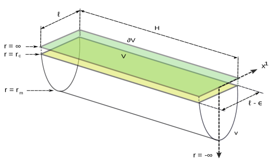
Figure 1: (Colour Online) The strip $V$ in the asymptotic boundary, with the minimal surface $v$ in the bulk ending on $\partial V$. The entangling surface $\partial V$ consists of two flat (hyper)planes positioned at $x^{1}=\ell/2$ and $x^{1}=-\ell/2$. A regulator length $H$ is introduced to limit the extent of these planes along the remaining directions.

Now let us begin to consider evaluating the holographic entanglement entropy for a general RG flow. As in the previous section, we assume the bulk metric takes the form given in eq. (6). Then the boundary geometry is simply flat space and we define the entangling surfaces as follows: First recall that the entangling surface divides a Cauchy surface (e.g., the constant time slice, $x^{0}=t=0$) into two regions. As described above, we wish to consider an interval of length $\ell$ and so we introduce two flat (hyper)planes at $x^{1}=\ell/2$ and $x^{1}=-\ell/2$, as shown in figure 1. We also introduce a regulator length $H$ to limit the size of the two planes along the $x^{2,3,\cdots,d-1}$ directions, e.g., we can imagine the boundary is periodic in these directions with length $H\gg\ell$. Hence the area of either plane is $H^{d-1}$, as described at eq. (25). In calculating the holographic entanglement entropy, we consider bulk surfaces that end on the entangling surface as $r\to\infty$, as shown in figure 1. With the ‘slab’ geometry described here, the radial profile of these surfaces will only be a function of the coordinate $x=x^{1}$. We will write the profile as $r=r(x,w=\ell)$ where $w$ indicates the width of the interval which sets the boundary condition, i.e., in the present case, $x\to\ell/2$ as $r\to\infty$. Of course, the holographic calculations are only well-defined if we introduce an asymptotic cut-off surface as some $r=r_{c}$. The position of this surface is related to a short distance cut-off in the boundary theory, i.e., $r_{c}=\tilde{L}\,\log(\tilde{L}/\delta)$. The radial profile will define another useful UV scale $\epsilon$ with $r_{c}=r(x=(\ell-\epsilon)/2,w=\ell)$, i.e., the profile intersects the cut-off surface $r=r_{c}$ at $x=(\ell-\epsilon)/2$. Another useful scale in the bulk surface is the minimal radius $r_{m}$ which it reaches in the bulk, which appears as $r_{m}=r(x=0,w=\ell)$.

Given the background metric (6) and our ansatz $r(x,\ell)$ for the profile of the bulk surface, we find that eq. (29) reduces to the following simple expression

$$S={2\pi\over\ell_{\textrm{\tiny P}}^{d-1}}\int_{m}d^{d-1}x\,\frac{e^{(d-2)A}\left(e^{2A}+\left(1+2\,\lambda L^{2}\,A^{\prime}{}^{2}\right)\dot{r}^{2}\right)}{\sqrt{e^{2A}+\dot{r}^{2}}}\,.$$ (30)

where $\dot{r}=\partial r/\partial x$ and $A^{\prime}=dA/dr$. Now one may treat the above expression as an action which is varied to find a second-order differential equation to determine the profile $r(x,\ell)$. However, since the integrand above has no explicit dependence on the coordinate $x$, the following is a conserved quantity along the radial profile

$${K_{d}(\ell)}\,\equiv\,{e^{-dA}\,(e^{2A}+\dot{r}^{2})^{3/2}\over e^{2A}+(1-2\,\lambda L^{2}\,A^{\prime}{}^{2})\,\dot{r}^{2}}\,.$$ (31)

This leaves us with a first-order equation for the profile, which should be easier to solve. In principle then, our goal is to solve for $r(x,\ell)$ in a given holographic RG flow geometry, i.e., for a specific conformal factor $A(r)$, and then substitute the solution back into eq. (30) to calculate the entanglement entropy.

Before going on to consider the entanglement entropy and c-function for RG flow geometries, let us first examine the results when the bulk geometry is simply AdS space, i.e., at a fixed point of the flow where the boundary theory is conformal. Recall that for the AdS vacuum $A(r)=r/\tilde{L}$. Let us begin by setting $\lambda=0$ and considering the results for Einstein gravity in the bulk. The case of three-dimensional AdS or a $d=2$ boundary CFT is special since the entanglement entropy yields a logarithmic UV divergence

$$S_{\textrm{\tiny CFT}}\;=\;{4\,\pi\tilde{L}\over\ell_{\textrm{\tiny P}}}\,\log\left({\ell\over\delta}\right)\,.$$ (32)

If we recall that the central charge of the boundary CFT is given by $c=12\pi\,\tilde{L}/\ell_{\textrm{\tiny P}}$, we see that this expression precisely reproduces the expected result (3) for the entanglement entropy of a two-dimensional CFT. Next turning to Einstein gravity with $d\geq 3$, the entanglement entropy for the interval is given by [45]

$$S_{\textrm{\tiny CFT}}\;=\;\frac{4\pi}{d-2}\,{\tilde{L}^{d-1}\over\ell_{\textrm{\tiny P}}^{d-1}}\left({H\over\delta}\right)^{d-2}-{2^{d}\,\pi^{(d+1)/2}\,\over(d-2)}\left({\Gamma({d\over 2(d-1)})\over\Gamma({1\over 2(d-1)})}\right)^{d-1}\,{\tilde{L}^{d-1}\over\ell_{\textrm{\tiny P}}^{d-1}}\,\left(H\over\ell\right)^{d-2}\,.$$ (33)

Here we see the general structure given in eq. (25) with two terms, a power law divergence proportional to $(H/\delta)^{d-2}$ and a finite contribution proportional to $(H/\ell)^{d-2}$. Next for $\lambda=0$, both of the central charges in eqs. (16) and (17) are identical and we use this fact to define $\mathcal{C}_{d}$ in eq. (25) for Einstein gravity: $\mathcal{C}_{d}(\lambda=0)\equiv\pi^{d/2}/\Gamma(d/2)\,(\tilde{L}/\ell_{\textrm{\tiny P}})^{d-1}=C_{T}=a_{d}^{*}$. As described previously then, we can extract this central charge from the above entanglement entropy using eq. (26), which yields

$$\mathcal{C}_{d}=\beta_{d}\,\frac{\ell^{d-1}}{H^{d-2}}\,\frac{\partial S_{\textrm{\tiny CFT}}}{\partial\ell}\quad{\rm with}\ \ \beta_{d}=\frac{1}{\sqrt{\pi}\,2^{d}\,\Gamma(d/2)}\left(\Gamma({1\over 2(d-1)})\over{\Gamma({d\over 2(d-1)})}\right)^{d-1}\,.$$ (34)

Hence we have identified the precise value of $\beta_{d}$ (for $d\geq 3$) which appears as the coefficient in eq. (27) of the c-function.

Finally let us apply the above formulae to calculate holographic entanglement entropy with the strip geometry for the boundary CFT dual to the AdS vacuum in GB gravity (12). To simplify the final results, it is convenient to first treat $r$ as the independent variable, in which case to fix the profile of the bulk surface, we must determine $x(r)$. Next we choose a new radial coordinate $\tau=K^{-1/(d-1)}\,e^{-r/\tilde{L}}$ and define $h\equiv e^{2r/\tilde{L}}\,(\partial_{r}x)^{2}$. Note that as $r\to\infty$, $\tau\to 0$ and further one can show at $r=r_{m}$, $\tau=1$. Now with these choices, eq. (31) becomes

$$\frac{\tau^{d-1}\,(1+h)^{3/2}}{\sqrt{h}\,(1-2\lambda f_{\infty}+h)}=1\,.$$ (35)

In general, this equation yields three roots for $h(\tau)$ and the relevant solution is the real root which can be continuously connected to the $\lambda=0$ solution: $h=\tau^{2(d-2)}/(1-\tau^{2(d-2)})$. Now it is straightforward to see that the entanglement entropy (30) can be written as

$$S_{\textrm{\tiny CFT}} \;=\; {4\pi\over d-2}\left(1+2\lambda f_{\infty}\right){\tilde{L}^{d-1}\over\ell_{\textrm{\tiny P}}^{d-1}}\left({H\over\delta}\right)^{d-2}-\frac{4\pi}{d-2}\left(1+2\lambda f_{\infty}\right){\tilde{L}^{d-1}\over\ell_{\textrm{\tiny P}}^{d-1}}\left({H\over\ell}\right)^{d-2}$$ (36)

$$\qquad\times\ I^{d-2}\,\Bigg{[}1+(d-2)\int_{0}^{1}\frac{d\tau}{\tau^{d-1}}\Bigg{(}1-{1+2\lambda f_{\infty}+h\over\left(1+2\lambda f_{\infty}\right)\sqrt{1+h}}\Bigg{)}\Bigg{]}\,,$$

where $I\equiv\int_{0}^{1}d\tau\sqrt{h}$. Then applying eq. (34), we can express the central charge in the finite contribution as

$$\mathcal{C}_{d}(\lambda) \;=\; 4\pi\beta_{d}\left(1+2\lambda f_{\infty}\right){\tilde{L}^{d-1}\over\ell_{\textrm{\tiny P}}^{d-1}}\,I^{d-2}\,\Bigg{[}1+(d-2)\int_{0}^{1}\frac{d\tau}{\tau^{d-1}}\Bigg{(}1-{1+2\lambda f_{\infty}+h\over\left(1+2\lambda f_{\infty}\right)\sqrt{1+h}}\Bigg{)}\Bigg{]}\,.$$ (37)

Regrettably, we do not have a closed analytic expression for $\mathcal{C}_{d}(\lambda)$ in terms of the two central charges $C_{T}$ and $a_{d}^{*}$. Hence we have numerically evaluated the above expression and plotted $\mathcal{C}_{d}(\lambda)/a_{d}^{*}$ as a function of $C_{T}/a_{d}^{*}$ in figure 2a for several values of $d$. Note that in this figure, $\mathcal{C}_{d}(\lambda)/a_{d}^{*}=1$ at $C_{T}/a_{d}^{*}=1$ for all of the values of $d$ since this corresponds to $\lambda=0$ or Einstein gravity in the bulk. From these curves, we can infer that $\mathcal{C}_{d}(\lambda)$ is a complicated nonlinear function of both $C_{T}$ and $a_{d}^{*}$. We can also illustrate this fact as follows: In the vicinity of $\lambda\simeq 0$ or $C_{T}\simeq a_{d}^{*}$, we can make a linearized analysis of eq. (37) to find

$$\mathcal{C}_{d}(\lambda)=\mathcal{C}_{d}(0)\left(1+{3(d-1)\over 2}\lambda+O(\lambda^{2})\,\right)=\mathcal{C}_{L}(\lambda)+O(\lambda^{2})$$ (38)

where

$$\mathcal{C}_{L}(\lambda)\equiv\frac{(d-1)(d-2)}{2}\,C_{T}+\frac{d(d-3)}{2}\,a_{d}^{*}\,.$$ (39)

Here, we have defined $\mathcal{C}_{L}(\lambda)$ as the linear combination of the two central charges in eqs. (16) and (17) which yields an $O(\lambda)$ expansion which precisely matches that for $\mathcal{C}_{d}(\lambda)$. Next, we consider the ratio of $\mathcal{C}_{d}(\lambda)$ and $\mathcal{C}_{L}(\lambda)$ over the full (physical) range of $\lambda$. Since $\mathcal{C}_{L}(\lambda)$ can vanish in this range, it is convenient plot the ratio $\mathcal{C}_{L}(\lambda)/\mathcal{C}_{d}(\lambda)$ as a function of $C_{T}/a_{d}^{*}$, as shown in figure 2b. This figure illustrates even more dramatically our previous observation that $\mathcal{C}_{d}(\lambda)$ is a complicated nonlinear function of both $C_{T}$ and $a_{d}^{*}$. At this point, let us add that since $\mathcal{C}_{d}(\lambda)\neq a_{d}^{*}$, the central charge identified in [20] as satisfying a c-theorem, we might not expect that our new effective central charge $\mathcal{C}_{d}(\lambda)$ will always flow monotonically in holographic RG flows for general $\lambda$.

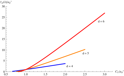
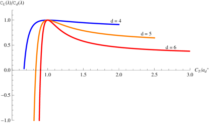
(a)	(b)

Figure 2: (Colour Online) Panel (a) plots $\mathcal{C}_{d}(\lambda)/a_{d}^{*}$ as a function of $C_{T}/a_{d}^{*}$ for GB gravity, while panel (b) is a plot of $\mathcal{C}_{L}(\lambda)/\mathcal{C}_{d}(\lambda)$ as a function of $C_{T}/a_{d}^{*}$. Note that both $\mathcal{C}_{d}(\lambda)/a_{d}^{*}=1=\mathcal{C}_{L}(\lambda)/\mathcal{C}_{d}(\lambda)$ at $C_{T}/a_{d}^{*}=1$ which corresponds to Einstein gravity in the bulk (i.e., $\lambda=0$). Each curve runs over the physically allowed range of $C_{T}/a_{d}^{*}$ for the given value of $d$ — see eq. (18) for more details.

4 Holographic flow of c-function with Einstein gravity

In this section, we examine the behavior of the c-function (27) in a general holographic RG flow dual to Einstein gravity. We will first discuss the flow of the c-function in $d=2$ and then generalize it to arbitrary dimensions.

For $d=2$, the bulk theory is three-dimensional Einstein gravity coupled to, e.g., a scalar field with a nontrivial potential, as described in section 2. Our holographic expression (30) for the entanglement entropy of a strip can be written as

$$S\,=\,{4\pi\over\ell_{\textrm{\tiny P}}}\int_{0}^{\frac{\ell-\epsilon}{2}}dx\,\sqrt{\dot{r}^{2}+e^{2A}}\,.$$ (40)

Note that the integration above runs over half of the range, i.e., $x\in[\,0,(\ell-\epsilon)/2\,]$. Further the conserved charge (31) simplifies to

$$K_{2}(\ell)\,=\,e^{-2A(r)}\,\sqrt{\dot{r}^{2}+e^{2A}}\,.$$ (41)

To calculate $dS/d\ell$, we note that $\dot{r}=\dot{r}(x,\ell)$ and $A=A(r(x,\ell))$, i.e., the profile of the extremal surface implicitly depends on the strip width $\ell$. If we vary $S$ with respect to $\ell$, keeping the UV cut-off $r=r_{c}$ fixed, we will get two contributions: one coming from change in the limits of the integration and second from change in the solution $r(x,\ell)$. We write them as

$${dS\over d\ell}\,=\,{4\,\pi\over\ell_{\textrm{\tiny P}}}{1\over\sqrt{\dot{r}^{2}+e^{2A(r)}}}\left[{1\over 2}\left(1-{d\epsilon\over d\ell}\right)(\dot{r}^{2}+e^{2A(r)})+\dot{r}\,{\partial r\over\partial\ell}\right]\Bigg{|}_{x={\ell-\epsilon\over 2}}\,,$$ (42)

where we have used the equation of motion for $r(x,\ell)$

$$\ddot{r}-A^{\prime}\,\left(2\dot{r}^{2}+e^{2A}\right)\,=\,0\,,$$ (43)

to cancel the bulk contribution. Since the UV cut-off $r_{c}$ is fixed while performing the variation, we get some extra constraints between $\dot{r}=\partial_{x}r$ and $r^{\prime}=\partial_{\ell}r$ at the asymptotic boundary. Taking variation of relation $r({\ell-\epsilon\over 2},\ell)=r_{c}$ with respect to $\ell$, we get

$$\left[{\dot{r}(x,\ell)\over 2}\left(1-{d\epsilon\over d\ell}\right)+{\partial r(x,\ell)\over\partial\ell}\right]_{x={\ell-\epsilon\over 2}}\,=\,0\,.$$ (44)

Substituting this relation, as well as eq. (41), into eq. (42) gives us following expression for $dS/d\ell$:

$${dS\over d\ell}\,=\,-{4\pi\over\ell_{\textrm{\tiny P}}\,K_{2}(\ell)}{1\over\dot{r}}{\partial r\over\partial\ell}\bigg{|}_{x={\ell-\epsilon\over 2}}\,.$$ (45)

In the above relation, the partial derivatives of $r(x,\ell)$ are evaluated near the asymptotic boundary. To further simplify this expression, we use the Fefferman-Graham expansion near the boundary [30]. In terms of the radial coordinate $r$, this expansion takes the form [24]

$$ds^{2}\,=\,dr^{2}+e^{{2r/{\tilde{L}}}}\,f(r)\,\eta_{ij}\,dx^{i}\,dx^{j}\,,$$ (46)

where

$$f(r)\,=\,1+a_{1}\phi_{0}^{2}\,e^{-2\alpha r/\tilde{L}}+a_{3}\phi_{0}^{3}\,e^{-3\alpha r/\tilde{L}}+\cdots\;.$$ (47)

In this expansion, $\tilde{L}$ is the AdS radius in the UV region (i.e., as $r\to\infty$) and $\alpha=d-\Delta$ where $\Delta$ is the conformal weight of the operator dual to the bulk scalar field. Near the boundary, the coordinate $r$ is very large and hence it is sufficient to work with only the leading order term in the expansion (47). Although $A(r)$ has a complicated profile deep inside the bulk, near the boundary it will have the simple form

$$A(r)\,=\,{r/{\tilde{L}}}\,.$$ (48)

For this $A(r)$, eq. (41) can be re-expressed as the following equation of motion: $dx/dr=e^{-2r/\tilde{L}}/\sqrt{K_{2}^{2}-e^{-2r/\tilde{L}}}$. The latter is easily integrated to yield the following solution

$$x-{\ell\over 2}\,=\,\tilde{L}\sqrt{K_{2}^{2}-e^{-2r/\tilde{L}}}-\tilde{L}K_{2}\,.$$ (49)

where the integration constant was chosen so that $x\to\ell/2$ as $r\to\infty$. Next we differentiate the above solution with respect to $x$ and $\ell$ to find $\dot{r}$ and $\partial r/\partial\ell$, treating that $K_{2}(\ell)$ as a function of $\ell$ – see appendix A for further details. Taking the limit $r\to\infty$ in ratio of $\partial r/\partial\ell$ and $\dot{r}$ appearing in eq. (45), we find that

$${1\over\dot{r}}{\partial r\over\partial\ell}\bigg{|}_{x=\ell/2}\,=\,-{1\over 2}\,.$$ (50)

This relation not only simplifies eq. (45) but also ensures that the first derivative of $S$ is indeed finite for all RG flow solutions. Using this relation in eq. (45), we arrive at following elegant form of the c-function (24) for arbitrary RG flow backgrounds:

$${c}_{2}\,=\,3\,\ell\,{dS\over d\ell}\,=\,{6\pi\over\ell_{\textrm{\tiny P}}}{\ell\over K_{2}(\ell)}\,.$$ (51)

The next step is to show that this c-function increases monotonically along holographic RG flows. Implicitly, the extremal bulk surfaces $v$ on which we are evaluating the Ryu-Takayanagi formula (28) extend to infinite $r$ at $x=\pm\ell/2$ and pass through a minimum $r=r_{m}$ at $x=0$. The latter radius gives us an indication of which degrees of freedom the entanglement entropy is probing, i.e., for smaller values of $r_{m}$, we expect the entropy and $c_{2}$ responds more to the IR structure of the RG flow. Hence in the following, we will study behavior of ${c}_{2}$ as a function of the turning point radius $r_{m}$ and we wish to establish the ‘c-theorem’ as $dc_{2}/dr_{m}\geq 0$ – at least for background geometries that satisfy appropriate constraints.

Comparing to the field theory construction of [2], we note that there the c-theorem was formulated as $dc_{2}/d\ell\leq 0$. Naively, this result matches with the holographic inequality which we wish to establish since we expect that as the width of the strip increases, the minimal area surface will explore deeper regions in the bulk geometry. The two inequalities would be rigorously connected if we could prove a second inequality $d\ell/dr_{m}\leq 0$ for consistent holographic models. However, as we will see in the next section, in fact this inequality does not hold for all extremal surfaces. However, we will still find $dc_{2}/d\ell\leq 0$ in all cases of interest. The violations of the previous inequality are associated with unstable saddle-points which do not contribute to the physical entanglement entropy. Hence, in section 5, we will find that the behaviour of the entanglement entropy in general holographic RG flows provides a richer story than might have been naively anticipated.

Returning to the flow of the c-function, we note that at the minimum of the bulk surface, we will have $r(0,\ell)=r_{m}$ and $\dot{r}(0,\ell)=0$. Hence considering eq. (41) at this turning point, we find

$$K_{2}(r_{m})\,=\,e^{-A(r_{m})}\,.$$ (52)

Here it is natural to treat this constant of the motion as a function of $r_{m}$, rather than $\ell$. We will also work with width of the strip $\ell$ as function of $r_{m}$. Then combining eqs. (51) and (52) yields

$${d{c}_{2}\over dr_{m}}\,=\,{6\pi\over\ell_{\textrm{\tiny P}}K_{2}(r_{m})}\left({d\ell\over dr_{m}}+A^{\prime}(r_{m})\,\ell\right)\,.$$ (53)

Now to express $\ell$ in terms of $r_{m}$, we begin with the relation

$${\ell\over 2}\,=\,\int_{0}^{\ell/2}dx\,=\,\int_{r_{m}}^{\infty}{dr\over\dot{r}}\,=\,\int_{r_{m}}^{\infty}dr{e^{-2A}\,A^{\prime}\over\sqrt{K_{2}^{2}-e^{-2A}}}{1\over A^{\prime}}\,.$$ (54)

Here in the final expression we have used eq. (41). Now above, we will apply integration by parts using

$$\int dr\,\frac{e^{-2A}A^{\prime}}{\sqrt{K_{2}^{2}-e^{-2A}}}=\sqrt{K_{2}^{2}-e^{-2A}}\,.$$ (55)

to find that

$${\ell}\,=\,2\tilde{L}K_{2}+2\int_{r_{m}}^{\infty}dr{A^{\prime\prime}\over A^{\prime}{}^{2}}\sqrt{K_{2}^{2}-e^{-2A}}\,,$$ (56)

where we have used eq. (48) to evaluate $A^{\prime}(r)$ at $r=\infty$. Further we can differentiate this expression with respect to $r_{m}$ to get

$${d\ell\over dr_{m}}\,=\,-2\tilde{L}A^{\prime}(r_{m})\,K_{2}-2A^{\prime}(r_{m})\int_{r_{m}}^{\infty}dr{A^{\prime\prime}\over A^{\prime}{}^{2}}{K_{2}^{2}\over\sqrt{K_{2}^{2}-e^{-2A}}}\,.$$ (57)

Now substituting eqs. (56) and (57) into eq. (53), we find

$${d{c}_{2}\over dr_{m}} \,=\, -{12\,\pi A^{\prime}(r_{m})\over\ell_{\textrm{\tiny P}}\,K_{2}(r_{m})}\int_{r_{m}}^{\infty}dr{A^{\prime\prime}\over A^{\prime}{}^{2}}{e^{-2A}\over\sqrt{K_{2}^{2}-e^{-2A}}}\,$$

$$\,=\, -{12\,\pi A^{\prime}(r_{m})\over\ell_{\textrm{\tiny P}}\,K_{2}(r_{m})}\int_{0}^{\ell}dx\,{A^{\prime\prime}\over A^{\prime}{}^{2}}\,,$$ (58)

$$\,=\, -{12\,\pi A^{\prime}(r_{m})\over\ell_{\textrm{\tiny P}}\,K_{2}(r_{m})}\int_{0}^{\ell}dx\,{1\over A^{\prime}{}^{2}}\,\left(T^{t}{}_{t}-T^{r}{}_{r}\right)\geq 0\,.$$

In the second line, we have used eq. (41) to convert the integration over $r$ to one over $x$. In the last line, we have used Einstein’s equations to replace $A^{\prime\prime}$ by the components of the stress tensor. As for the discussion of holographic c-theorems in section 2, the final inequality assumes that the bulk matter fields driving the holographic RG flow satisfy the null energy condition. The latter ensures that the integrand is negative. The overall inequality also requires $K_{2}(r_{m})>0$ and $A^{\prime}(r_{m})>0$. The first condition is obvious from eq. (52) while the second can be established as follows: Given the null energy condition, it follows that $A^{\prime\prime}\leq 0$ which means that $A^{\prime}$ is everywhere a decreasing function of radial coordinate $r$. Implicitly, we are assuming the bulk geometry approaches AdS space asymptotically, i.e., the dual field theory approaches a conformal fixed point in the UV. Hence with $r\to\infty$, we see the minimal value of $A^{\prime}$ is $A^{\prime}=1/\tilde{L}$, where $\tilde{L}$ is the asymptotic AdS scale. Since this minimal value is positive, it must be that $A^{\prime}$ is positive everywhere along the holographic RG flow. Hence $d{c}_{2}/dr_{m}$ is positive and our two-dimensional c-function increases monotonically along the RG flow if the bulk matter satisfies the null energy condition.

We now turn to proving the monotonic flow of the c-function (27) for higher dimensions. The required analysis is a straightforward extension of the above calculations with $d=2$. In particular, one finds that eq. (51) generalizes to

$${c}_{d}\,=\,{2\,\pi\,\beta_{d}\over\ell_{\textrm{\tiny P}}^{d-1}}{\ell^{d-1}\over K_{d}(\ell)}\,,$$ (59)

with $d$ boundary dimensions. The conserved quantity (31) is now given by

$$K_{d}\,=\,e^{-dA(r)}\sqrt{\dot{r}^{2}+e^{2A(r)}}\,.$$ (60)

We have relegated the detailed derivation of eq. (59) to appendix A. However, we can see from this result that all the complexities of determining the c-function boil down to evaluating the conserved charge (60) for the minimal area surface. We might note that we can evaluate this expression at the minimal radius (where $\dot{r}=0$) to find

$$K_{d}(r_{m})=e^{-(d-1)A(r_{m})}\,,$$ (61)

which generalizes eq. (52) to general $d$.

Combining eqs. (59) and (61), we further find

$${d{c}_{d}\over dr_{m}}\,=\,{2\,(d-1)\pi\,\beta_{d}\,\ell^{d-2}\over K_{d}}\,\left(\frac{d\ell}{dr_{m}}+A^{\prime}(r_{m})\,\ell\right)\,.$$ (62)

To express $\ell$ in terms of $r_{m}$, eq. (54) now becomes

$${\ell\over 2}\,=\,\int_{0}^{\ell/2}dx\,=\,\int_{r_{m}}^{\infty}{dr\over\dot{r}}\,=\,\int_{r_{m}}^{\infty}dr{A^{\prime}\,e^{-dA(r)}\over\sqrt{K_{d}^{2}-e^{-2(d-1)A}}}{1\over A^{\prime}}\,,$$ (63)

where the last expression follows by using eq. (60). To make further progress, we observe that

$$\int dr\,{A^{\prime}\,e^{-dA(r)}\over\sqrt{K_{d}^{2}-e^{-2(d-1)A}}}=-{e^{-dA}\over d\,K_{d}}\ {}_{2}F_{1}\!\left[{1\over 2},{d\over 2(d-1)};{3d-2\over 2(d-1)};{e^{-2(d-1)A(r)}\over K_{d}^{2}}\right]$$ (64)

$$\quad=e^{-(d-2)A}\sqrt{K_{d}^{2}-e^{-2(d-1)A}}-\frac{e^{-(d-3)A}\,K^{2}_{d}}{\sqrt{K_{d}^{2}-e^{-2(d-1)A}}}\ {}_{2}F_{1}\!\left[{1\over 2},-{d-2\over 2(d-1)};{d\over 2(d-1)};{e^{-2(d-1)A(r)}\over K_{d}^{2}}\right]\,.$$

We have presented the second expression above to illustrate that this result is simply an extension of eq. (55) for general $d$ but in the following, we will use the more compact expression given in the first line. With eq. (64), we can integrate by parts in eq. (63) to find

$$\ell \,=\, {2\sqrt{\pi}\,K_{d}^{1/(d-1)}\over dA^{\prime}(r_{m})}\,{\Gamma\left({3d-2\over 2(d-1)}\right)\over\Gamma\left({2d-1\over 2(d-1)}\right)}$$

$$\qquad\qquad-2\int_{r_{m}}^{\infty}dr{A^{\prime\prime}\over A^{\prime}{}^{2}}{e^{-dA}\over d\,K_{d}}\ {}_{2}F_{1}\!\left[{1\over 2},{d\over 2(d-1)};{3d-2\over 2(d-1)};{e^{-2(d-1)A(r)}\over K_{d}^{2}}\right]\,.$$

Differentiating this result with respect to $r_{m}$ and making various simplifications yields

$${d\ell\over dr_{m}} \,=\, -{2\sqrt{\pi}\,K_{d}^{1/(d-1)}\over d}\,{\Gamma\left({3d-2\over 2(d-1)}\right)\over\Gamma\left({2d-1\over 2(d-1)}\right)}-2{A^{\prime}(r_{m})}\int_{r_{m}}^{\infty}dr\,{A^{\prime\prime}\over A^{\prime 2}}{e^{-dA}\over\sqrt{K_{d}^{2}-e^{-2(d-1)A}}}$$

$$\quad+2A^{\prime}(r_{m})\int_{r_{m}}^{\infty}dr\,{A^{\prime\prime}\over A^{\prime 2}}\,{e^{-dA}\over d\,K_{d}}\ {}_{2}F_{1}\!\left[{1\over 2},{d\over 2(d-1)};{3d-2\over 2(d-1)};{e^{-2(d-1)A(r)}\over K_{d}^{2}}\right]\,.$$

Now substituting eqs. (4) and (4) into eq. (62), we find

$${d{c}_{d}\over dr_{m}} \,=\, -{4\,\pi(d-1)\beta_{d}\,\ell^{d-2}\,A^{\prime}(r_{m})\over\ell_{\textrm{\tiny P}}^{d-1}\,K_{d}(r_{m})}\int_{r_{m}}^{\infty}dr\,{A^{\prime\prime}\over A^{\prime 2}}{e^{dA}\over\sqrt{K_{d}^{2}-e^{-2(d-1)A}}}$$

$$\,=\, -{4\,\pi(d-1)\beta_{d}\,\ell^{d-2}\,A^{\prime}(r_{m})\over\ell_{\textrm{\tiny P}}^{d-1}\,K_{d}(r_{m})}\int_{0}^{\ell}dx\,{A^{\prime\prime}\over A^{\prime 2}}$$ (67)

$$\,=\, -{4\,\pi\beta_{d}\,\ell^{d-2}\,A^{\prime}(r_{m})\over\ell_{\textrm{\tiny P}}^{d-1}\,K_{d}(r_{m})}\int_{0}^{\ell}dx\,{1\over A^{\prime 2}}\,\left(T^{t}{}_{t}-T^{r}{}_{r}\right)\geq 0\,.$$

The steps here are essentially the same as in our analysis of eq. (58) with $d=2$. The key requirement for the final inequality to hold is that the bulk matter fields driving the holographic RG flow must satisfy the null energy condition. With this assumption then, $d{c}_{d}/dr_{m}$ is positive and our $d$-dimensional c-function increases monotonically along the RG flow for holographic boundary theories dual to Einstein gravity in the bulk.

5 Explicit geometries and Phase transitions

In this section, we consider some simple bulk geometries describing holographic RG flows. This allows us to explicitly demonstrate that the c-function (27) indeed flows monotonically for boundary field theories dual to Einstein gravity. However, we will also find that for some RG flows, there is a ‘first order phase transition’ in the entanglement entropy as the width of the strip $\ell$ passes through a critical value. Technically, denoting the behaviour in the entanglement entropy as a phase transition is inappropriate – after all, the system itself, i.e., the state of the boundary field theory, does not change at all. However, as we will see below, in our holographic calculation of the entanglement entropy, there are competing saddle points and the dominant saddle point shifts at a critical value of the width. Of course, this behaviour is reminiscent of that seen in holographic calculations describing thermodynamic phase transitions [52] and so we adopt the nomenclature ‘phase transition’ to convey this picture. The phase transition is first order and so the entanglement entropy is continuous at the critical width $\ell_{t}$, however, the derivative $dS/d\ell$ is discontinuous at this point. As a result, the c-function drops discontinuously at the phase transition.

Implicitly, we are assuming that the holographic RG flows studied below are solutions of Einstein gravity and hence the entanglement entropy is determined by eq. (28). Explicitly, our RG flow geometries take the form given in eq. (6) and so are defined by giving the conformal factor $A(r)$. Here we note that in all of the examples we consider, $A^{\prime\prime}(r)\leq 0$ and so the geometry could solve Einstein’s equations with matter fields satisfying the null energy condition. In appendix C, we consider one approach to constructing an appropriate scalar field theory that could realize the latter. In any event with $A^{\prime\prime}(r)\leq 0$, the holographic c-theorem of section 4 will be satisfied. That is, $dc_{d}/dr_{m}\geq 0$ or alternatively, the c-function decreases monotonically as the corresponding extremal surface extends deeper into the bulk geometry, as will be shown below.

In general, we will consider arbitrary values of the boundary dimension in the following. However, to begin, we consider a very simple example of a step flow and the discussion will be limited to the case $d=2$, i.e., a three-dimensional bulk. The step profile consists of two AdS geometries with different curvature scales are patched together at some finite radius. With such a simple profile, the behaviour of the entanglement entropy and the c-function can be determined analytically. Our analysis with $d=2$ is easily extended to higher $d$ but we do not present the results here. In the subsequent subsection, we also examine smooth profiles describing an holographic RG flow and allow for arbitrary $d$. However, numerical analysis is required to understand the behaviour of the entanglement entropy for these smooth profiles.

5.1 Step profile

We limit the discussion here to three-dimensional gravity and consider a bulk geometry which patches together two AdS regions with different curvatures at some finite radius $r=r_{0}$. Using the metric ansatz in eq. (6), the conformal factor $A(r)$ is given by

$$A(r)=\bigg{\{}\begin{array}[]{l l l}A_{IR}(r)=\frac{r\,-\,r_{0}}{L_{IR}}+\frac{r_{0}}{L_{UV}}&\textrm{for }r\leq r_{0}&\\ A_{UV}(r)={r\over L_{UV}}&\textrm{for }r\geq r_{0}&\,,\end{array}$$ (68)

where $L_{UV}$ and $L_{IR}$ correspond to the AdS radius in the UV and IR regions, which we denote as AdS_UV and AdS_IR in the following. The constant term added to $A(r)$ in the IR region ensures that the conformal factor is continuous at $r=r_{0}$. Of course, it is not differentiable there and some stress energy with $\delta$-function support would be required to make this geometry a solution of Einstein’s equations. As discussed in previous sections, there is a conserved quantity (41) which plays an important role in determining to the entanglement entropy and the c-function. Clearly, there are two classes of minimal area surfaces in this geometry, namely those that stay only in AdS_UV and those that penetrate deep enough into the bulk so that the minimal radius $r_{m}$ is in AdS_IR. In either case, the conserved quantity $K_{2}$ is given by eq. (52) and hence we have $K_{UV}=e^{-A_{UV}(r_{m})}$ for $r_{m}\geq r_{0}$ and $K_{IR}=e^{-A_{IR}(r_{m})}$ for $r_{m}\leq r_{0}$. To regulate the entanglement entropy, all of these surfaces are terminated at a large cut-off radius $r=r_{c}$ in the UV region.

To find the minimal area surface, we will solve eq. (41) for $x=x(r)$. First, we can invert the latter equation to find

$${dx\over dr}\,=\,{e^{-2A(r)}\over\sqrt{K_{2}^{2}-e^{-2A(r)}}}\,.$$ (69)

Above we have discarded the root with an overall minus sign because we will only consider the branch of solutions covering the interval $x\in[0,\ell/2]$ in the following, for which $dx/dr\geq 0$. For the minimal surfaces that stay entirely in AdS_UV, we can easily integrate (69) to find

$$x\,=\,L_{UV}\sqrt{K_{UV}^{2}-e^{-2r/L_{UV}}}\,,$$ (70)

using $A_{UV}$ as given in eq. (68). The integration constant is chosen here so that $x=0$ at $r=r_{m}$, which also implies that

$$\ell=2L_{UV}K_{UV}=2L_{UV}e^{-r_{m}/L_{UV}}\,.$$ (71)

As noted above, this solution is valid for $r_{m}\geq r_{0}$, which implies $\ell\leq\ell_{2}$ where

$$\ell_{2}\equiv 2L_{UV}e^{-r_{0}/L_{UV}}\,.$$ (72)

Next we turn to the second class of minimal area surfaces, which penetrate into AdS_IR. In this case, we have $K_{2}=K_{IR}=e^{-A_{IR}(r_{m})}$ with the turning point $r_{m}$ in AdS_IR. We divide the relevant solutions of eq. (69) in two parts: $x_{IR}(r)\in[0,x_{t}]$ describes the portion of the extremal surface in AdS_IR and $x_{UV}(r)\in[x_{t},\ell/2]$ represents the part in AdS_UV. Here we have defined the transition point $x_{t}$ such that $x_{t}=x_{IR}(r_{0})=x_{UV}(r_{0})$. Now integrating eq. (69) with the appropriate conformal factor (68) for each segment, we find

$$x_{IR} \,=\, L_{IR}\sqrt{K_{IR}^{2}-e^{-2A_{IR}(r)}}$$

$$x_{UV} \,=\, L_{UV}\sqrt{K_{IR}^{2}-e^{-2A_{UV}(r)}}+{\ell\over 2}-L_{UV}K_{IR}\,.$$ (73)

Above, the integration constants were chosen so that $x_{IR}=0$ at $r=r_{m}$ and $x_{UV}=\ell/2$ as $r\to\infty$. Combining these solutions at $x_{IR}(r_{0})=x_{UV}(r_{0})=x_{t}$, we find

$$x_{t}\, = \,{L_{IR}\over L_{UV}-L_{IR}}\left(L_{UV}K_{IR}-{\ell\over 2}\right)\,,$$ (74)

$$\ell\, = \,2L_{UV}K_{IR}-2(L_{UV}-L_{IR})\sqrt{K_{IR}^{2}-e^{-2r_{0}/L_{UV}}}\,.$$ (75)

Here we have ensured that the solution (73) is continuous at $r=r_{0}$ but the first derivative is also continuous at this transition point because of the form of eq. (69) and the continuity of the conformal factor. Implicitly, eq. (75) gives the relation between $\ell$ and $r_{m}$ since $K_{IR}=e^{-A_{IR}(r_{m})}$. As the physically relevant quantity in the boundary theory is $\ell$, we invert this relation to find the following two solutions for $K_{IR}$:

$$K_{IR\pm}\,=\,{L_{UV}\ell\pm(L_{UV}-L_{IR})\sqrt{\ell^{2}-4L_{IR}(2L_{UV}-L_{IR})e^{-2r_{0}/L_{UV}}}\over 2L_{IR}(2L_{UV}-L_{IR})}\,.$$ (76)

Above, both of these roots provide real solutions for $\ell\geq\ell_{1}$ with

$$\ell_{1}\equiv 2\sqrt{L_{IR}(2L_{UV}-L_{IR})}\,e^{-r_{0}/L_{UV}}\,.$$ (77)

It is also useful to define $r_{1}$, the value of the minimum radius at $\ell=\ell_{1}$, for which we find

$$e^{-r_{1}/L_{IR}}\equiv\frac{L_{UV}}{\sqrt{L_{IR}(2L_{UV}-L_{IR})}}\,e^{-r_{0}/L_{IR}}\,.$$ (78)

Now the root $K_{IR+}$ is a monotonically increasing function of $\ell$ over the range $\ell_{1}\leq\ell\leq\infty$ and for any $\ell$ in this range, there is a consistent solution for the extremal surface. The corresponding values of the minimal radius are $r_{1}\geq r_{m}\geq-\infty$. Now the second root $K_{IR-}$ decreases for $\ell\sim\ell_{1}$, however, it is an increasing function for large values of $\ell$. $K_{IR-}$ has a single minimum at $\ell=\ell_{2}$, i.e., precisely the width defined in eq. (72) for the discussion of solutions remaining entirely in AdS_UV. At this minimum, $K_{IR-}$ takes the value $e^{-A_{IR}(r_{0})}=e^{-r_{0}/L_{UV}}$. We find that $K_{IR-}$ yields a consistent solution for the extremal surface as long as $\ell_{1}\leq\ell\leq\ell_{2}$. However, for $\ell>\ell_{2}$, the solutions corresponding to $K_{IR-}$ are inconsistent, e.g., $dx/dr$ is not positive throughout the range $x\in[0,\ell/2]$. We note that for the consistent solutions, while $\ell$ runs from $\ell_{1}$ to $\ell_{2}$, the minimum radius of these surfaces $r_{m}$ increases from $r_{1}$ to $r_{0}$. That is, in contrast to the previous two families of solutions, here we have $d\ell/dr_{m}>0$!

Hence the following picture has emerged for the extremal surfaces: Beginning with the minimal radius in the range $\infty>r_{m}\geq r_{0}$, there is a family of extremal solutions which remain entirely in AdS_UV. As can be seen from eq. (71), the width $\ell$ increases monotonically as $r_{m}$ decreases, reaching the maximum $\ell=\ell_{2}$ when $r_{m}=r_{0}$. Below this point, we make a transition to a new family of solutions which begin to penetrate into AdS_IR. For $r_{0}\geq r_{m}\geq r_{1}$, the relevant family of extremal surfaces corresponds to the branch with $K_{IR-}$. In this regime, $\ell$ actually decreases as $r_{m}$ continues to decrease, i.e., $d\ell/dr_{m}>0$. When $r_{m}$ reaches $r_{1}$, as given in eq. (78), $\ell=\ell_{1}$ and we make another transition to the third family of extremal surfaces. These solutions correspond to the branch with $K_{IR+}$. In this regime $r_{1}>r_{m}>-\infty$, $\ell$ again increases monotonically as $r_{m}$ decreases. Figure 3 illustrates this behaviour for all three families of extremal surfaces. Now for any particular value of the turning point radius $r_{m}$, we see there is unique extremal surface. However, if we consider the solutions as a function of the strip width $\ell$, there is a unique solution for $\ell<\ell_{1}$ and $\ell>\ell_{2}$. In the intermediate range $\ell_{1}\leq\ell\leq\ell_{2}$, there are in fact three possible extremal surfaces for any given width. Given three possible saddle points, we are instructed in eq. (28) to find the extremal surface with the minimum area in order to evaluate the entanglement entropy. This situation with multiple saddle points is also the typical scenario that one encounters in the holographic description of a thermodynamic phase transition [52] and in fact, we will find the latter extends to the present situation. That is, we see below that the entanglement entropy undergoes a ‘first order phase transition’.

Figure 3: (Colour Online) This plot illustrates the behaviour of $\ell$ as a function of $r_{m}$ for all three families of extremal surfaces. The red, blue and green portions of the curve correspond to the contributions coming from $S_{IR}(K_{IR+})$, $S_{IR}(K_{IR-})$ and $S_{UV}$, respectively. In particular, we see that $d\ell/dr_{m}\leq 0$ for $S_{IR}(K_{IR+})$ and $S_{UV}$, while $d\ell/dr_{m}\geq 0$ for $S_{IR}(K_{IR-})$. For this plot, we chose $L_{UV}=1$, $L_{IR}=0.1$ and $r_{0}=0$.

Hence having found the solutions for the extremal surfaces, we will present an entropy, i.e., $S=2\pi A(v)/\ell_{\textrm{\tiny P}}$, for each of these surfaces. But, of course, in the intermediate regime described above, the true entanglement entropy is given by the solution which minimizes this quantity. Let us begin with the solutions (70) which remain entirely in AdS_UV. For this case, the entropy turns out to be

$$S_{UV}\,=\,{4\pi L_{UV}\over\ell_{\textrm{\tiny P}}}\,\log\left({\ell\over\delta}\right)+\mathcal{O}(\delta)\,.$$ (79)

Here the result is expressed in terms of a short-distance cut-off in the boundary theory $\delta$, which is related to the radial cut-off by

$$r_{c}=L_{UV}\,\log\left(L_{UV}/\delta\right)\,.$$ (80)

Now let us consider the extremal surfaces given by eqs. (73) to (76), which penetrate into AdS_IR. For this case, the calculation of entanglement entropy results

$$S_{IR}\, =\,{4\pi\over\ell_{\textrm{\tiny P}}}\int_{0}^{x_{t}}dx\,\sqrt{e^{2A_{IR}(r)}+\dot{r}^{2}}+{4\pi\over\ell_{\textrm{\tiny P}}}\int_{x_{t}}^{(\ell-\epsilon)/2}dx\,\sqrt{e^{2A_{UV}(r)}+\dot{r}^{2}}$$ (81)

$$=\,\frac{2\pi L_{IR}}{\ell_{\textrm{\tiny P}}}\log\left[\frac{L_{IR}K_{IR}+x_{t}}{L_{IR}K_{IR}-x_{t}}\right]+\frac{2\pi L_{UV}}{\ell_{\textrm{\tiny P}}}\log\left[\frac{4L_{UV}K_{IR}-\epsilon}{4L_{UV}K_{IR}-\ell+2x_{t}}\,\frac{\ell-2x_{t}}{\epsilon}\right]\,.$$

We convert the cut-off $\epsilon$ above to $\delta$ using $r(x=(\ell-\epsilon)/2,\ell)=r_{c}$, which yields

$$\epsilon\,\simeq\,{\delta^{2}\over L_{UV}K_{IR}}\,.$$ (82)

Using this relation, we can write

$$S_{IR} \,=\, \frac{4\pi L_{UV}}{\ell_{\textrm{\tiny P}}}\log\left[\frac{2L_{UV}K_{IR}}{\delta}\right]+\frac{2\pi L_{IR}}{\ell_{\textrm{\tiny P}}}\log\left[\frac{L_{IR}K_{IR}+x_{t}}{L_{IR}K_{IR}-x_{t}}\right]$$ (83)

$$\qquad\qquad\qquad\qquad\qquad-\frac{2\pi L_{UV}}{\ell_{\textrm{\tiny P}}}\log\left[\frac{4L_{UV}K_{IR}-\ell+2x_{t}}{\ell-2x_{t}}\right]\,.$$

This result is valid for both of the roots $K_{IR\pm}$ given in eq. (76).

Now as described above, the UV family of solutions (70) provide the unique extremal surface for any $\ell<\ell_{1}$ and hence the entanglement entropy is given by $S=S_{UV}$ in this regime. Similarly, for $\ell>\ell_{2}$, the extremal surface is again unique and hence the entanglement entropy is given by $S=S_{IR}(K_{IR+})$. In the intermediate regime $\ell_{1}\leq\ell\leq\ell_{2}$, we have three extremal surfaces and we must identify which of these yields the minimal entropy. In particular, we always find $S_{IR}(K_{IR+})\leq S_{IR}(K_{IR-})$ and hence the branch with $K_{IR-}$ never plays a role in determining the physical entanglement entropy. Therefore the latter is found by comparing $S_{UV}$ and $S_{IR}(K_{IR+})$. It turns out that these two entropies are equal for some critical width $\ell_{t}$ with $\ell_{1}\leq\ell_{t}\leq\ell_{2}$. Further $S_{UV}>S_{IR}(K_{IR+})$ for $\ell>\ell_{t}$ and $S_{UV}<S_{IR}(K_{IR+})$ for $\ell<\ell_{t}$. Hence we find that, the entanglement entropy for the step profile (68) is given by

$$S\,=\,\left\{\begin{array}[]{l l}S_{UV}(\ell)&\textrm{for }\ell\leq\ell_{t}\\ S_{IR}(K_{IR+}(\ell))&\textrm{for }\ell\geq\ell_{t}\,,\end{array}\right.$$ (84)

with $\ell_{t}$ defined by $S_{UV}(\ell_{t})=S_{IR}(K_{IR+}(\ell_{t}))$. In particular, we observe that the entanglement entropy exhibits a first order phase transition at the critical width $\ell=\ell_{t}$. Further, we note that at transition, $S(\ell)$ is continuous but not differentiable. We have illustrated all of this behaviour in figure 4, which plots $S(\ell)-S(\ell_{2})$ versus $\log(\ell/\ell_{2})$ for specific values of the parameters, $L_{UV}$, $L_{IR}$ and $r_{0}$, defining the profile.

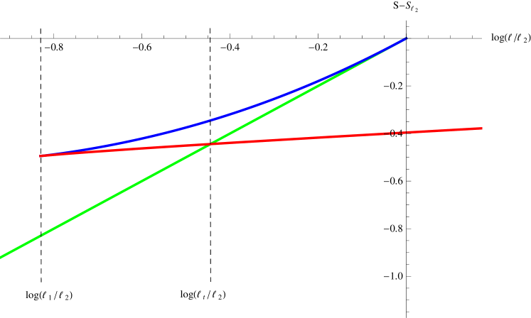
Figure 4: (Colour Online) This plot illustrates the entropy for all three families of extremal surfaces as a function of the width of the strip $\ell$. The green curve corresponds to $S_{UV}$; the red, to $S_{IR}(K_{IR-+})$; and the blue, to $S_{IR}(K_{IR-})$. The phase transition occurs at $\ell=\ell_{t}$ where the red and green curves cross. For this plot, we have chosen $L_{UV}=1$, $L_{IR}=0.5$ and $r_{0}=0$.

Given the entanglement entropy (84), we turn to the calculation of the c-function defined in eq. (24). We could proceed here by explicitly differentiating the various expressions above, e.g., eq. (83), with respect to $\ell$ to determine $c_{2}$. However, this calculation only verifies the final result which was already determined in our general analysis in section 4, namely eq. (51). In fact, this result applies for all three families of extremal surfaces and so we have

$${c}_{2}\,=\,\left\{\begin{array}[]{l l}{6\pi\over\ell_{\textrm{\tiny P}}}{\ell\over K_{UV}}&\textrm{from }S_{UV}\\ {6\pi\over\ell_{\textrm{\tiny P}}}{\ell\over K_{IR-}}&\textrm{from }S_{IR}(K_{IR-})\\ {6\pi\over\ell_{\textrm{\tiny P}}}{\ell\over K_{IR+}}&\textrm{from }S_{IR}(K_{IR+})\,,\end{array}\right.$$ (85)

where $K_{UV}=\ell/(2L_{UV})$ and $K_{IR\pm}$ are given in eq. (76). Figure 5a plots $c_{2}$ as a function of the turning point radius – or rather $e^{r_{m}/L_{UV}}$. We see that $d{c}_{2}/dr_{m}\geq 0$ everywhere in the figure, which is again in keeping with the expectations of our general analysis in section 4. However, because of the phase transition, not all values of $r_{m}$ are relevant for the c-function (24) evaluated on the physical entanglement entropy (84). In figure 5a, the region between the vertical dashed lines is excluded and the physical c-function jumps discontinuously between the values at the points labeled $A$ and $B$. This behaviour is also illustrated in figure 5b where the c-function in eq. (85) is plotted as a function of the ratio $\ell/\ell_{t}$. The phase transition at $\ell=\ell_{t}$ again takes $c_{2}$ between the points labeled $A$ and $B$, which now lie on the same vertical dashed line in this figure. That is, at this critical value of the strip width, the c-function drops from the value given by $S_{UV}$ (on the green curve) to that given by $S_{IR}(K_{IR+})$ (on the red curve). Again this discontinuity arises because of the first order nature of the phase transition, i.e., the entanglement entropy is continuous but not differentiable at this point. If we consider only the physical values of $c_{2}$, then we also find $d{c}_{2}/d\ell\leq 0$ in keeping with the general expectations of field theory analysis of [2]. Of course, figure 5b also illustrates that $d{c}_{2}/d\ell>0$ on the branch associated with $K_{IR-}$. However, as emphasized above, this family of saddle points is not relevant of the physical entanglement entropy (84). The ‘unusual’ behaviour of the c-function on this branch arises because $d\ell/dr_{m}\geq 0$ for this family of solutions. Given the behaviour illustrated by this simple example, it seems likely that in general any branch of extremal surfaces with the latter property will correspond to unstable saddle points which are not physically relevant.

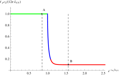
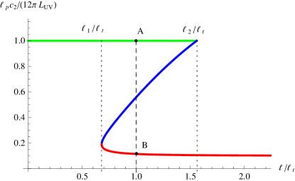
(a)	(b)

Figure 5: (Colour Online) Panel (a) plots the c-function (85) as a function of $e^{-r_{m}/L_{UV}}$. This plot clearly illustrates that $c_{2}$ decreases monotonically as $r_{m}$ decreases, in accord with the analysis of section 4. However, the region between the vertical dashed lines is excluded by the phase transition in the entanglement entropy. Rather the physical c-function jumps from the point labeled A to that labeled B. Panel (b) plots the c-function with respect to $\ell/\ell_{t}$. One can see that $c_{2}$ is multi-valued in the region $\ell_{1}\leq\ell\leq\ell_{2}$, as noted in eq. (85). Again at $\ell=\ell_{t}$, the c-function drops discontinuously between the points labeled A and B. The red, blue and green portions of both curves correspond to the contributions coming from $S_{IR}(K_{IR+})$, $S_{IR}(K_{IR-})$ and $S_{UV}$, respectively. For this plot, we chose $L_{UV}=1$, $L_{IR}=0.1$ and $r_{0}=0$.

5.2 Smooth profiles

The simple example in the previous section has alerted us to the possibility that the entanglement entropy $S(\ell)$ may experience a phase transition with respect to changing the strip width $\ell$. However, one should worry that this result is an artifact of the artificial shape of the step profile in eq. (68). Hence we consider some smooth profiles in this section and examine to what extent this phase transition survives for these more realistic holographic RG flows. Again our definition of the holographic entanglement entropy is given in eq. (28) and so implicitly we are assuming that the bulk geometry is a solution of Einstein’s equations. In appendix C, we consider the scalar field theory that would be necessary to realize the latter. In this section, we will consider arbitrary values of the boundary dimension $d$.

Let us first consider a smooth flow between the UV and IR fixed points with the following conformal factor

$$e^{A(r)}\,=\,e^{r/L}\,\big{(}2\cosh\!\left({r/R}\right)\big{)}^{-\gamma}\,,$$ (86)

Notice that $A(r)\simeq r/L-\gamma r/R$ in the limit $r\to+\infty$ and $A(r)\simeq r/L+\gamma r/R$ for $r\to-\infty$. Hence the geometry approaches AdS space in both of these limits with

$${1\over L_{UV}}\,\equiv\,{1\over L}-\frac{\gamma}{R}\quad\textrm{and}\quad{1\over L_{IR}}\,\equiv\,{1\over L}+\frac{\gamma}{R}\,.$$ (87)

The parameter $R$ controls the sharpness of the transition in the holographic flow between the UV and IR fixed points while the change in the AdS scale is controlled by the combination $\gamma/R$. In the limit $R\to 0$ with $\gamma/R$ fixed, we would recover a step profile of the form given in eq. (68).

To proceed further in examining the possibility of a phase transition, we used the analysis presented in previous sections and examined the extremal surfaces numerically for the above holographic flow profile. First, using eq. (60), the equation determining the shape of the extremal surfaces is reduced to a first order equation,

$${dx\over dr}\,=\,{e^{-dA(r)}\over\sqrt{K_{d}^{2}-e^{-2(d-1)A(r)}}}\,.$$ (88)

as appears in eq. (69) for $d=2$. Then families of surfaces are easily constructed as a function of the turning point radius $r_{m}$ using eq. (61). Numerically integrating from the turning point out to the asymptotic region, we can then determine $\ell(r_{m})$.

Let us add a few more details about the numerical analysis: Near $r=r_{m}$, one finds that $x\sim\sqrt{r-r_{m}}$ and hence eq. (88) is singular precisely at $r=r_{m}$, the putative starting point of our numerical integration. So to simplify the numerical analysis, we define

$$y(r)=\sqrt{r-r_{m}}\,x(r)\,,$$ (89)

for which the equation of motion (88) becomes

$${dy\over dr}\,=\,{y\over 2(r-r_{m})}+{\sqrt{r-r_{m}}\,e^{-dA(r)}\over\sqrt{K_{d}^{2}-e^{-2(d-1)A(r)}}}\,.$$ (90)

With this new coordinate, $y\sim(r-r_{m})$ near $r=r_{m}$ and the right hand side of the equation of motion (90) is finite. To set the initial conditions, we use eq. (90) to find the leading terms in a series expansion of $y(r)$ in $r-r_{m}$. Now we can numerically integrate eq. (90) out from the turning point $r=r_{m}$ to large asymptotic values of $r$ and find the the strip width $\ell$ using the relation

$$\ell\,=\,\lim_{r\to\infty}{2\,y(r)\over\sqrt{r-r_{m}}}\,.$$ (91)

Now as discussed previously, the appearance of a phase transition is directly related to the appearance of a regime where $d\ell/dr_{m}>0$. Figure 6 illustrates that such behaviour still arises for a range of parameters in the smooth profile (86). However, as shown in the figure when $R$ grows (holding $\gamma/R$ fixed), this region decreases and eventually $d\ell/dr_{m}<0$ for all values of $r_{m}$. That is, there exists a critical value $R_{c}$ such that, for $R<R_{c}$ there is a first order phase transition while for $R>R_{c}$, we observe a smooth cross-over. At precisely $R=R_{c}$, there is a single point where $d\ell/dr_{m}=0$ and the slope is otherwise negative. In this case, the phase transition would be second order.

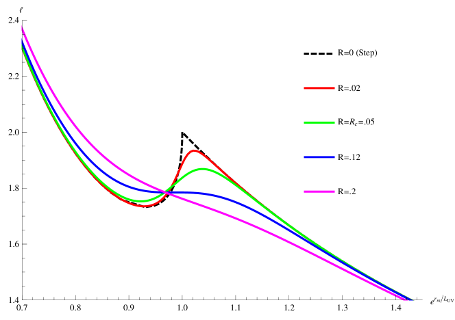
Figure 6: (Colour Online) Plot of strip width $\ell$ as a function of $e^{r_{m}/L_{UV}}$ for various values of the profile width $R$. With small $R$, there is a regime where $d\ell/dr_{m}>0$. However, for large $R$, $d\ell/dr_{m}<0$ everywhere. There is a critical value $R_{c}$ for which $d\ell/dr_{m}$ reaches zero at a single point and is otherwise negative. The plot was prepared using the smooth profile (86) with $L=0.66$ and $\gamma=0.5R$, as well as $d=2$. These parameter values yield $L_{IR}=0.5$ and $L_{UV}=1$.

Of course, one can go beyond the above analysis to identify the precise point where the phase transition occurs given specific values of the parameters in eq. (86) which produce a regime where $d\ell/dr_{m}>0$. Hence for some range of the width $\ell$, there will be multiple surfaces which locally extremize the entropy functional (124). Determining which surface provides the dominant saddle point requires carefully regulating the entanglement entropy and comparing the values of finite parts of entropy for the competing saddle points. This analysis is essentially the same as in section 5.1, however, in the present case with a smooth conformal factor, the profile $x(r)$ and the entropy integral are evaluated numerically. We will not present any of these results here.

Let us now turn to the asymptotic expansion of the profile (86) and compare it to the Fefferman-Graham (FG) expansion given in eqs. (46) and (47). We find that

$$f(r)\,=\,\left(1+e^{-2r/R}\right)^{-\gamma}\simeq 1-\gamma e^{-2r/R}+\dots\,.$$ (92)

which yields $\alpha=L_{UV}/R$ in eq. (47). Now as described in section 2, the natural holographic interpretation of this flow would be that the UV fixed point is perturbed by a relevant operator, which would be dual to by a scalar field in the bulk theory. However, as discussed in appendix C, applying this interpretation to the bulk solution yields an upper bound on the parameter $\alpha$ appearing in the FG expansion (47), i.e., $\alpha\leq{d\over 2}+1$. This bound then becomes a constraint on $R$, the width of the holographic profile (86). That is,

$$R\geq{2L_{UV}\over d+2}\,.$$ (93)

Previously we found that the smooth holographic RG flows described by eq. (86) will still yield a first order phase transition in the entanglement entropy provided the width is sufficiently small, i.e., $R\leq R_{c}$. Hence the lower bound given in eq. (93) creates a certain tension. Namely, if $R_{c}$ does not satisfy this lower bound, it seems likely that the phase transition is still an artifact of the artificial shape of the profile in eq. (86). We examine this question in figure 7a, where we have plotted $(d+2)R_{c}/2L_{UV}$ for different values of $L_{UV}/L_{IR}$. The bound (93) implies that $(d+2)R/2L_{UV}>1$ and as the figure illustrates, the latter can only be satisfied for sufficiently large $d$, i.e., $d\geq 6$. Hence the possibility of a phase transition is called into question for the physical dimensions $d=2,3,4$.

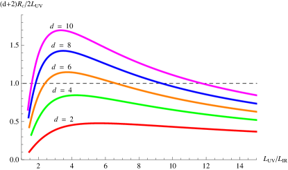
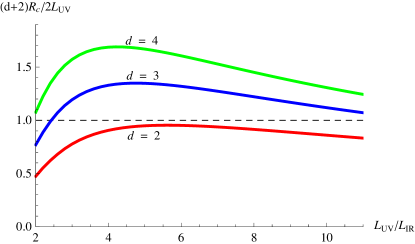
(a)	(b)

Figure 7: (Colour Online) Panel (a) plots ${(d+2)R_{c}\over 2L_{UV}}$ as a function of ${L_{UV}\over L_{IR}}$ for various dimensions with the two-parameter conformal factor (86). Eq. (93) implies ${(d+2)R_{c}\over 2L_{UV}}>1$ for a consistent interpretation of the holographic RG flow. Panel (b) plots ${(d+2)R_{c}\over 2L_{UV}}$ as a function of ${L_{UV}\over L_{IR}}$ for the three-parameter conformal factor (94) with $\sigma=5\times 10^{-4}$.

Now the profile (86) was constructed to give a simple example which would smooth out the step potential studied in the previous subsection. One can easily generalize this profile to include more independent parameters and study the effect on the phase transition. Hence as another simple example, we consider the following conformal factor

$$e^{A(r)}\,=\,e^{r/L}\left(e^{2r/R}+2\sigma+e^{-2r/R}\right)^{-\gamma/2}\,.$$ (94)

Of course, if one chooses $\sigma=1$, this profile reduces to the previous one in eq. (86). Hence the AdS scales in the UV and IR limits are again given by eq. (87) with the new expression. However, in this case, the sharpness of the transition between the asymptotic UV and IR geometries is effectively controlled by both $R$ and $\sigma$. Given this new profile, we can readily extend the previous analysis to find in which parameter regime $(R,\sigma)$ the entanglement entropy undergoes a phase transition. We do not present any details but a qualitative observation is that $R_{c}$ becomes larger with smaller values of $\sigma$. Now considering the FG expansion in this case, the metric function in eq. (47) becomes

$$f(r)\,=\,\left(1+2\sigma e^{-2r/R}+e^{-4r/R}\right)^{-\gamma/2}=1-\gamma\,\sigma\,e^{-2r/R}+\dots\,.$$ (95)

Hence we still have $\alpha=L_{UV}/R$ and the lower bound in eq. (93) remains unchanged. Hence, as shown in figure 7b, we find that $R_{c}$ can now satisfy this bound for $d\geq 3$. Our expectation is that by further embellishing the form of the holographic RG flow profile, we can also find realistic geometries, i.e., geometries satisfying eq. (93), which produce a phase transition in the entanglement entropy for $d=2$ as well.

6 Holographic flow of c-function with GB gravity

In this section, we return to examining the general behaviour of the c-function (27) in holographic RG flows but now where the bulk geometries are solutions of GB gravity (12). As noted in section 3.1, the calculation of holographic entanglement entropy in GB gravity requires that we extremize the entropy functional given in eq. (29) [49, 23]. Evaluating this functional for the strip geometry yields the expression in eq. (30). The extremal surfaces are again characterized by a conserved quantity which now takes the form given in eq. (31). The latter is most simply evaluated by considering the turning point of the extremal surface where $r=r_{m}$ and $\dot{r}=0$ so that eq. (31) yields

$$K_{d}(r_{m})\,=\,e^{-(d-1)A(r_{m})}\,,$$ (96)

precisely as was found before for Einstein gravity.

Recall that with Einstein gravity, we found a simple relation between $K_{d}$ and $dS/d\ell$ – see eq. (135). In the following, we will show that this same relation extends to GB gravity. To simplify the discussion, we denote the integrand in eq. (30) as $\mathcal{L}$ and then $K_{d}$ can be expressed as

$${1\over K_{d}(\ell)}\,=\,\mathcal{L}-{d\mathcal{L}\over d\dot{r}}\dot{r}\,.$$ (97)

Now we vary the entanglement entropy functional (30) with respect to the width of the strip $\ell$ to find

$${dS_{GB}\over d\ell}\,=\,{4\pi H^{d-2}\over\ell_{\textrm{\tiny P}}^{d-1}}\left[{1\over 2}\left(1-{d\epsilon\over d\ell}\right)\mathcal{L}\Big{|}_{x={\ell-\epsilon\over 2}}+\int_{0}^{{\ell-\epsilon\over 2}}dx\left({\delta\mathcal{L}\over\delta r}\,{\partial r\over\partial\ell}+{\delta\mathcal{L}\over\delta\dot{r}}\,{\partial\dot{r}\over\partial\ell}\right)\right]\,.$$ (98)

Note that there is an extra overall factor of $2$ above to since we are only integrating over half of the bulk surface, i.e., from the turning point $(x,r)=(0,r_{m})$ to the boundary $(x,r)=((\ell-\epsilon)/2,r_{c})$. Now surfaces extremizing eq. (30) will satisfy

$${\delta\mathcal{L}\over\delta r}={\partial\over\partial x}\left({\delta\mathcal{L}\over\delta\dot{r}}\right)\,.$$ (99)

Further eq. (44) still applies in the present analysis and so allows us to express $(1-d\epsilon/d\ell)$ in terms of derivatives of the profile $r(x,\ell)$. With both of these expressions, we are able to simplify eq. (98) to take the form

$${dS_{GB}\over d\ell} \,=\, {4\pi H^{d-2}\over\ell_{\textrm{\tiny P}}^{d-1}}\left[-{\mathcal{L}\over\dot{r}}\,{\partial r\over\partial\ell}\Big{|}_{x={\ell-\epsilon\over 2}}+\left[{d\mathcal{L}\over d\dot{r}}{\partial r\over\partial\ell}\right]_{x=0}^{{\ell-\epsilon\over 2}}\right]$$ (100)

$$\,=\, -{4\pi H^{d-2}\over\ell_{\textrm{\tiny P}}^{d-1}K_{d}(\ell)}{1\over\dot{r}}\,{\partial r\over\partial\ell}\bigg{|}_{x={\ell-\epsilon\over 2}}\,.$$

Here the boundary term at $x=0$ vanishes because $\dot{r}=0$ there. Eq. (97) was then used to simplify the remaining terms with $K_{d}(\ell)$. We note that precisely the same expression as above appeared in the analysis of $dS/d\ell$ with Einstein gravity – see eq. (129).

The next step is to show that the ratio ${1\over\dot{r}}{\partial r\over\partial\ell}$ has the same simple boundary limit as found previously in eq. (134) with Einstein gravity. The analogous procedure would call for solving eq. (31) to find $\dot{r}$. However, in the present case, we would find a cubic equation in $\dot{r}^{2}$ and which would in general have six distinct roots. The relevant root would be that which in the limit $\lambda\to 0$ is continuously connected to the solution (133) found with Einstein gravity. While it is possible to carry out this procedure analytically, it is not very illuminating. Rather we note that we are interested in the behaviour near the asymptotic boundary where the geometry approaches AdS space and the conformal factor takes the form $A(r)=r/\tilde{L}$. Now it is sufficient to expand near the boundary where $e^{A}$ is very large and the leading contribution to $\dot{r}$ becomes

$$\dot{r}\,\simeq\,e^{dr/\tilde{L}}\,K_{d}\,\left(1-2\lambda f_{\infty}\right)\,\,.$$ (101)

This equation is easily solved to yield $x(r)$ near the boundary. Of course, the integration constant is chosen to satisfy the boundary condition $x(r\to\infty)\to\ell/2$. Using this asymptotic solution for the profile of the extremal surface, it is easy to confirm that

$${1\over\dot{r}}{\partial r\over\partial\ell}\bigg{|}_{x=\ell/2}\,=\,-{1\over 2}\,,$$ (102)

as desired. Note that this relation is independent of the GB coupling $\lambda$.

Substituting eq. (102) into eq. (100), we arrive at

$${dS_{GB}\over d\ell}\,=\,{2\pi H^{d-2}\over\ell_{\textrm{\tiny P}}^{d-1}}{1\over K_{d}(\ell)}\,,$$ (103)

which precisely matches the expression (135) found with Einstein gravity. It seems that this result is quite general. The first key ingredient is, of course, the conserved quantity (97). The other necessary ingredient is that the asymptotic geometry approaches AdS space, which seems sufficient to produce the simple expression in eq. (102). Hence we expect that the expression (103) should be general to all cases with these two basic features.

Next, we turn to the flow of c-function (27) as we change the minimum radius $r_{m}$ of the extremal surfaces, as considered for Einstein gravity in section 4. Given eq. (103), our starting point for the c-function (27) is precisely the same as in eq. (59), i.e.,

$${c}_{d}\,=\,{2\,\pi\,\beta_{d}\over\ell_{\textrm{\tiny P}}^{d-1}}{\ell^{d-1}\over K_{d}(\ell)}\,,$$ (104)

Hence using eq. (96), we find

$${d{c}_{d}\over dr_{m}}\,=\,{2\,\pi(d-1)\beta_{d}\ell^{d-2}\over\ell_{\textrm{\tiny P}}^{d-1}K_{d}}\left({d\ell\over dr_{m}}+A^{\prime}(r_{m})\,\ell\right)\,.$$ (105)

Following our previous analysis, we express $\ell$ in terms of $r_{m}$ with

$${\ell\over 2} \,=\, \int_{r_{m}}^{\infty}{dr\over\dot{r}}\,=\,\int_{r_{m}}^{\infty}dr{1\over A^{\prime}}{A^{\prime}\over\dot{r}}\,.$$ (106)

However, in the present case, it is not possible to use the explicit root from eq. (31) for $\dot{r}$ and perform the integral. Hence we define

$$F(r,r_{m})\,=\,-\int^{\infty}_{r}dr{A^{\prime}\over\dot{r}}\,,$$ (107)

and use integration by parts in eq. (106) to write

$${\ell\over 2} \,=\, \left[{1\over A^{\prime}}F(r,r_{m})\right]_{r_{m}}^{\infty}+\int_{r_{m}}^{\infty}dr{A^{\prime\prime}\over A^{\prime 2}}F(r,r_{m})$$

$$\,=\, -{F(r_{m},r_{m})\over A^{\prime}(r_{m})}+\int_{r_{m}}^{\infty}dr{A^{\prime\prime}\over A^{\prime 2}}F(r,r_{m})\,.$$ (108)

In eq. (107), we have chosen the above limits on integration because the integrand vanishes at the asymptotic boundary $r=\infty$. Further, the dependence on $r_{m}$ in eq. (107) comes from $\dot{r}(x,r_{m})$. We should remind the reader that in the following discussion, our independent parameters are the profile $r(x,\ell)$ and $r_{m}$. Now differentiating eq. (108), we find

$${1\over 2}{d\ell\over dr_{m}} \,=\, -{1\over\dot{r}}\bigg{|}_{r_{m}}-{1\over A^{\prime}(r_{m})}{\partial\over\partial r_{m}}F(r,r_{m})\bigg{|}_{r_{m}}+\int_{r_{m}}^{\infty}dr{A^{\prime\prime}\over A^{\prime 2}}{\partial\over\partial r_{m}}F(r,r_{m})\,.$$ (109)

The first term above arises since ${\partial F(r,r_{m})/\partial r}=A^{\prime}(r)/\dot{r}$ but note that this term should be evaluated slightly away from $r=r_{m}$ since $\dot{r}=0$ there. This potential divergence will be canceled below by a contribution which is revealed in the second term below. Now substituting eqs. (108) and (109) into eq. (105), we find

$${d{c}_{d}\over dr_{m}}\,=\,{4\,\pi(d-1)\beta_{d}\,\ell^{d-2}\over\ell_{\textrm{\tiny P}}^{d-1}K_{d}}\left(I_{1}-I_{2}\right)\,,$$ (110)

where

$$I_{1} \,=\, \int_{r_{m}}^{\infty}dr{A^{\prime\prime}\over A^{\prime}{}^{2}}{\partial\over\partial r_{m}}F(r,r_{m})+A^{\prime}(r_{m})\int_{r_{m}}^{\infty}dr{A^{\prime\prime}\over A^{\prime 2}}F(r,r_{m})$$

$$\,=\, -A^{\prime}(r_{m})\int_{r_{m}}^{\infty}dr{A^{\prime\prime}\over A^{\prime}{}^{2}}\left[\int^{\infty}_{r}d\tilde{r}\,{A^{\prime}(\tilde{r})\over\dot{\tilde{r}}^{2}}\left(\dot{\tilde{r}}+(d-1)K_{d}{\partial\dot{\tilde{r}}\over\partial K_{d}}\right)\right]$$ (111)

and

$$I_{2} \,=\, {1\over\dot{r}}\bigg{|}_{r_{m}}+{1\over A^{\prime}(r_{m})}{\partial\over\partial r_{m}}F(r,r_{m})\bigg{|}_{r_{m}}+F(r_{m},r_{m})$$

$$\,=\, {1\over\dot{r}}\bigg{|}_{r_{m}}-\int^{\infty}_{r_{m}}dr\,{A^{\prime}\over\dot{r}^{2}}\left(\dot{r}+(d-1)K_{d}{\partial\dot{r}\over\partial K_{d}}\right)\,.$$ (112)

In writing these expressions, we have used $\partial\dot{r}/\partial r_{m}=(\partial\dot{r}/\partial K_{d})(dK_{d}/dr_{m})$, as well as eq. (96). Now considering the local expression for $K_{d}$ in eq. (31), we calculate $\partial\dot{r}/\partial K_{d}$ keeping $r$ fixed. Similarly, we can differentiate eq. (31) with respect to $x$, which yields an expression involving $\ddot{r}$. We find that these two quantities are related by the following:

$$\dot{r}\,A^{\prime}\left(\dot{r}+(d-1)K_{d}\,{\partial\dot{r}\over\partial K_{d}}\right)\,=\,\ddot{r}+4\lambda L^{2}\,A^{\prime}\,A^{\prime\prime}\,\dot{r}^{2}\,Q$$ (113)

where

$$Q\,\equiv\,{\dot{r}^{2}+e^{2A}\over\dot{r}^{2}\,(1-2\,\lambda L^{2}A^{\prime}{}^{2})+e^{2A}(1+4\,\lambda L^{2}\,A^{\prime}{}^{2})}\,.$$ (114)

We now use eq. (113) to express eqs. (111) and (112) as

$$I_{1} \,=\, -A^{\prime}(r_{m})\int_{r_{m}}^{\infty}{dr\over\dot{r}}{A^{\prime\prime}\over A^{\prime}{}^{2}}-4\lambda L^{2}\,A^{\prime}(r_{m})\int_{r_{m}}^{\infty}dr\,{A^{\prime\prime}\over A^{\prime}{}^{2}}\left[\int^{\infty}_{r}d\tilde{r}\,{A^{\prime}(\tilde{r})\,A^{\prime\prime}(\tilde{r})\over\dot{\tilde{r}}}\,Q(\tilde{r})\right]\,,$$

$$I_{2} \,=\, 4\lambda L^{2}\,\int_{\infty}^{r_{m}}dr\,{A^{\prime}\,A^{\prime\prime}\over\dot{r}}\,Q\,,$$ (115)

where we have used $\int dr\,\ddot{r}/\dot{r}^{3}=-\int dx\,\partial/\partial x(1/\dot{r})=-1/\dot{r}$. Now inserting these expression (115) into eq. (110) and then integrating by parts, we arrive to following result

$${d{c}_{d}\over dr_{m}} \,=\, -{4\,\pi(d-1)\beta_{d}\,\ell^{d-2}\,A^{\prime}(r_{m})\over\ell_{\textrm{\tiny P}}^{d-1}\,K_{d}(r_{m})}\int_{r_{m}}^{\infty}dr\,{A^{\prime\prime}\over\dot{r}A^{\prime}{}^{2}}\left(1-4\lambda L^{2}\,A^{\prime 2}Q\right)$$ (116)

$$\,=\, -{4\,\pi\beta_{d}\,\ell^{d-2}\,A^{\prime}(r_{m})\over\ell_{\textrm{\tiny P}}^{d-1}\,K_{d}(r_{m})}\int_{0}^{\ell}dx\,{1\over A^{\prime}{}^{2}}\left(T^{t}{}_{t}-T^{r}{}_{r}\right)\,\frac{1-4\lambda L^{2}\,A^{\prime 2}Q}{1-2\lambda L^{2}\,A^{\prime 2}}$$

Here we used the GB equations of motion, i.e., eq. (147), to replace $A^{\prime\prime}$ by various components of the matter stress tensor. Note that the final result matches that in eq. (67) when $\lambda=0$. However, with $\lambda\neq 0$, it is clear that the null energy condition alone (which ensures $T^{t}{}_{t}-T^{r}{}_{r}\leq 0$) is insufficient to enforce a definite sign for $d{c}_{d}/dr_{m}$. Rather we must also be able to make a clear statement about the positivity of the last factor in the integral, i.e.,

$$\frac{1-4\lambda L^{2}\,A^{\prime 2}Q}{1-2\lambda L^{2}\,A^{\prime 2}}\,=\,{\dot{r}^{2}\,(1-6\,\lambda L^{2}A^{\prime}{}^{2})+e^{2A}\over(1-2\lambda L^{2}\,A^{\prime 2})(\dot{r}^{2}\,(1-2\,\lambda L^{2}A^{\prime}{}^{2})+e^{2A}(1+4\,\lambda L^{2}\,A^{\prime}{}^{2}))}\,.$$ (117)

As described above, one could use eq. (31) to express $\dot{r}^{2}$ in terms of the conserved charge $K_{d}$ and the conformal factor $A$, however, the resulting expression for eq. (117) is lengthy and unilluminating. In the limit of small $\lambda$ we observe that eq. (117) becomes

$$\frac{1-4\lambda L^{2}\,A^{\prime 2}Q}{1-2\lambda L^{2}\,A^{\prime 2}}\,\simeq\,1-2\,\lambda L^{2}A^{\prime}{}^{2}+\cdots\,.$$ (118)

Hence it is not clear what simplification one might expect in eq. (116). However, this result is still suggestive in that it is easy to see that the right hand side is positive as long as $\lambda<0$. Unfortunately, examining the full expression in eq. (117), we see that this simple condition does not quite guarantee that this factor is positive. Thus while we have an expression for $d{c}_{d}/dr_{m}$ in GB gravity, we are not able to make a simple statement of the conditions that are necessary to ensure that the c-function flows monotonically along holographic RG flows.

7 Discussion

With eq. (27), we constructed a simple extension to higher dimensions of the c-function (24) considered in ref. [2] for two-dimensional quantum field theories. As described in section 3, while the entanglement entropy itself contains a UV divergence, this expression (27) is finite and, at conformal fixed points, yields a central charge that characterizes the underlying conformal field theory, as had been noted previously in [23, 46]. In section 4, we examined the behaviour of this c-function in holographic RG flows in which the bulk theory was described by Einstein gravity. In particular, we were able to show that the flow of the c-function was monotonic as long as the matter fields driving the holographic RG flow satisfied the null energy condition. As reviewed in section 2, the latter condition was precisely the constraint that appears in the standard derivation of the holographic c-theorem [18, 19, 20].

We observe that if the bulk geometry is such that it ‘slightly’ violates the null-energy condition over a ‘small’ radial regime, the integral in eqs. (58) or (67) would remain positive and hence the flow of our c-function would still be monotonic. That is, we only need the null energy condition to be satisfied in some averaged sense. Hence the null-energy condition is a sufficient but not a necessary condition for the monotonic flow of the c-function (27). Thus there is less sensitivity to the bulk geometry is the present construction of a holographic c-theorem using the entanglement entropy than in the original discussions [18, 19]. It is intriguing that when expressed as an integral over the boundary direction $x$, eq. (67) weights the contributions of the bulk stress tensor more or less equally for each interval $\delta x$ in the strip. However, when the integral is expressed as an integral over the radial direction, the integrand includes an extra factor or $1/\dot{r}$, which diverges at the minimum radius $r_{m}$ of the holographic surface (but the integral remains finite). Hence in the holographic flows, the c-function responds sensitively to changes in the geometry near this radius in the bulk – a result that can be seen in the explicit flows discussed in section 5. Hence given the holographic connection between radius in the bulk and energy scales in the boundary theory, it seems clear that the flow of this c-function is most sensitive to the lowest energy modes probed by the entanglement entropy.

Our result for the monotonic flow of c-function in section 4 refers to the derivative $dc_{d}/dr_{m}$, i.e., changes in $c_{d}$ as we change the minimum energy scale probed by the entanglement entropy. To describe the flow of $c_{d}$ completely in terms of the boundary theory, we would actually like to establish $dc_{d}/d\ell\leq 0$, i.e., the c-function decreases monotonically as we increase the width of the strip for which the entanglement entropy is evaluated. In this case, we would be using the width $\ell$ as a proxy for the relevant energy scale along the RG flow. The desired result can be established in the present holographic framework, however, as discussed in section 5, one must be careful to restrict attention to the physical saddle points in evaluating the entanglement entropy. We showed there that extremal surfaces can arise for which $d\ell/dr_{m}>0$ and hence $dc_{d}/d\ell>0$. However, these saddle points do not contribute when one evaluates the holographic entanglement entropy with eq. (28) since they are never the minimum area surface. Rather the appearance of these ‘unstable’ saddle points signals a first order ‘phase transition’ in the entanglement entropy. As a result, $c_{d}$ drops discontinuously at some critical value $\ell_{t}$ of the width of the strip and the monotonic ‘flow’ of the c-function is preserved.

While we have only illustrated this behaviour with specific examples in section 4, it seems clear that the physical entanglement entropy will never be determined by such saddle points. In particular, if we are studying a holographic RG flow between two AdS geometries, we will always find $d\ell/dr_{m}<0$ when $r_{m}$ is well into either of these two asymptotic regions. Hence as argued in section 5.2, if extremal surfaces arise for which $d\ell/dr_{m}>0$, it indicates that there are a number of competing saddle points in the corresponding regime. First $\ell(r_{m})$ is a single-valued function since the conserved charge (31) dictates that there is a unique surface for each value of $r_{m}$. Hence if we assume this is a smooth function, there will always be (at least) three competing saddle points when $d\ell/dr_{m}>0$. It then becomes inevitable that there will be a phase transition in the corresponding regime of $\ell$. Further we note that

$$\frac{dS\ }{dr_{m}}=\frac{H^{d-2}}{\ell^{d-1}}\,\frac{c_{d}}{\beta_{d}}\,\frac{d\ell\ }{dr_{m}}\,.$$ (119)

The first two factors above are positive definite and hence the sign of $dS/dr_{m}$ is controlled entirely by $d\ell/dr_{m}$. Given this result, it is straightforward to argue that the behaviour illustrated in figure 4 is in fact generic. That is, the phase transition goes between the two branches for which $d\ell/dr_{m}<0$. Hence we have argued that given $dc_{d}/dr_{m}\geq 0$, it also follows that $dc_{d}/d\ell\leq 0$ for RG flows dual to Einstein gravity.

One may be concerned that the phase transitions noted above are an artifact of choosing a background geometry in the bulk which is unphysical in some way. However, with our analysis in section 5 and appendix C, we argued that the phase transitions can arise for holographic backgrounds that have a natural interpretation as an RG flow in the boundary theory, but also for backgrounds where the interpretation seems to be more exotic. While this interpretation was explicitly shown to apply in examples of phase transitions with the boundary dimension $d\geq 3$, constructing further examples to extend this result to $d=2$ does not seem difficult. However, we note that these phase transitions are undoubtedly effect of the large $N$ limit which is implicit in our constructions. However, it may still be that similar behaviour, i.e., rapid transitions in the entanglement entropy, persists in the RG flows of more conventional physical systems. In any event, it would be interesting to better understand these phase transitions in the holographic systems. Such a transition seems to indicate that quantum correlations in underlying degrees of freedom change dramatically at some particular energy scale in the RG flow.

It is worthwhile noting that phase transitions in the holographic entanglement entropy of the kind found here and in [26] for RG flows also arise in a variety of other holographic constructions. The simplest example is to consider the case where the entangling surface contains two disjoint regions. When the two regions are relatively close together, saddle point determining the holographic entanglement entropy will be a single connected bulk surface. However, as the two regions are moved apart, there is a phase transition to a second saddle point consisting of two separate bulk surfaces [47]. A similar phase transition was also found in considering the holographic entanglement entropy of the strip geometry for a bulk background corresponding to a confining phase of the boundary theory [54, 55]. There is a strong similarity between the results for these confining theories and the present RG flows since the phase transition again arises as the width to the strip passes through some critical value and results in a discontinuous drop in the central charge $c_{d}$. Further, in both cases, the phase transition can be interpreted as being produced by a rapid and drastic restructuring in the correlations of the low energy degrees of freedom (in comparison to high energy correlations). Similar results were also found for other entangling geometries, i.e., a circular surface in three-dimensional confining boundary theory [56]. Finally similar phase transitions in the entanglement entropy have also been found in holographic superconductors as the temperature is varied [57] and in the time evolution of holographic quantum quenches [58].

In section 6, we considered extending our results to holographic models where the gravitational theory in the bulk is Gauss-Bonnet gravity (12). While it is straightforward to construct an expression (116) for $d{c}_{d}/dr_{m}$ in GB gravity, it is evident that the null energy condition is not sufficient to guarantee a monotonic flow of the c-function. Unfortunately, eq. (116) does not lend itself to a simple statement of the conditions that would necessary to ensure that the c-function flows monotonically along holographic RG flows in these models. Further insight into this question may be provided by examining explicit holographic RG flows. In section 5, we assumed that the holographic backgrounds were solutions of Einstein gravity and hence the entanglement entropy is determined by eq. (28). We could just as easily assume that the same backgrounds are solutions of GB gravity and examine the behaviour of the c-function defined by eq. (29). In particular, it would be interesting to see if there are violations of the monotonic flow of the c-function in certain parameter regimes.

Of course, it may not be a surprise that the monotonic flow of the c-function (27) is not directly connected to the null energy condition in GB gravity. As described in section 2, an important feature of this theory is that at conformal fixed points, the dual boundary theory has two distinct central charges, given in eqs. (16) and (17). Using the null energy condition, ref. [20] established that the charge denoted $a_{d}^{*}$ would satisfy a c-theorem in these holographic models. However, in section 3, we found that the c-function (27) actually corresponds to a nonlinear combination of both central charges. Hence as we noted at the outset, it was improbable that a simple holographic c-theorem could be established for GB gravity with the present construction. Setting holography aside, it is known that for four-dimensional quantum field theories, there is no possible (linear) combination of the two central charges, $c=C_{T}$ and $a=a_{d}^{*}$, that can satisfy a c-theorem other than $a$ alone [8].

Of course, GB gravity only provides an interesting extension of the usual holographic framework for $d\geq 4$. For smaller values of $d$, the curvature-squared interaction (13) does not contribute to the gravitational equations of motion because of the topological origin of this term. It may be of interest to study the behaviour of our c-function for other gravity theories with higher curvature interactions for $d=2$ and 3. Interesting families of holographic models were considered with higher curvature theories of the three-dimensional gravity in [53]. A defining feature of these theories was that the dual $d=2$ boundary theory should exhibit a c-theorem. Hence these models may provide an interesting holographic framework to examine the RG flow of $c_{2}$. However, the work of [2] indicates that this flow must be monotonic for any unitary and Lorentz invariant quantum field theory and so confirming this result here would really be a test that these holographic models define reasonable boundary theories.

Our construction of the c-function (27) can be applied quite generally, i.e., outside of the context of holography. While the RG flow of $c_{d}$ is not expected to be monotonic in a generic setting, we observe that the flow can be constrained somewhat following the analysis of [2]. In particular, let us define a new (dimensionful) function of the following form in arbitrary $d$:

$$\hat{c}_{d}\,\equiv\,\frac{c_{d}}{\ell^{d-2}}\,=\,{\beta_{d}\over H^{d-2}}\ell{dS\over d\ell}\,.$$ (120)

Of course, for $d=2$, we have $\hat{c}_{2}=c_{2}$. In any event, we can apply directly the analysis of [2] to show that $d\hat{c}_{d}/d\ell\leq 0$ for any $d$. There, the authors considered unitary and Lorentz invariant field theories and used sub-additivity of the entanglement entropy to show that $\hat{c}_{2}$ is a monotonically decreasing function as $\ell$ increases. In particular, they considered two specific surfaces $b$ and $c$ with a relative boost, as shown in figure 8. Further $a$ and $d$ chosen as constant time surfaces in some frame so that they are Cauchy surfaces whose causal development corresponds to the intersection and union of the causal development of the original two boosted surfaces. By construction the surfaces $a$, $b$ and $c$ just touch the boundary of the causal development of $d$ on either end. Two important observations are: First, if we are evaluating the entanglement entropy for these segments in the Lorentz invariant vacuum state, then it should only depend on the proper length of the corresponding interval. Second, the entanglement entropy of any of these surfaces will be the same as for any other Cauchy surface of the corresponding domains since the time evolution is assumed to be unitary. Now the authors of [2] show that sub-additivity of the entanglement entropy of these regions imposes the following relation

$$S(b)-S(a)\geq S(\alpha b)-S(\alpha a)\,,$$ (121)

where they introduce the ratio of the proper lengths $\alpha=c/a=d/b\geq 1$. Now if the relative boost is taken to be small, this relation implies that $\ell\,dS/d\ell=c_{2}/3=\hat{c}_{2}/3$ must decrease with increasing $\ell$. Now these elegant arguments can also be applied without change in considering the entanglement entropy for the strip geometry in arbitrary dimensions, as long as the boundaries of the strip are orthogonal to the boost direction. That is, the segments $a$, $b$, $c$ and $d$ in figure 8 now represent the orthogonal cross-section of four specific strips. Hence with the previous arguments, we will recover the relation (121) for arbitrary dimensions. This implies that with the strip geometry in arbitrary dimensions, we have $d\hat{c}_{d}/d\ell\leq 0$ — the same observation was made in [54]. While we cannot conclude that the original c-function (27) must decrease with increasing $\ell$, using eq. (120), we find an upper bound on the rate at which ${c}_{d}$ could increase:

$$\ell\,{d{c}_{d}\over d\ell}\,\leq\,(d-2)\,{c}_{d}\,.$$ (122)

This bound applies to any $d$-dimensional quantum field theory, subject to the provisos of Lorentz invariance, unitarity and sub-additivity of entanglement entropy.

Figure 8: Here the boosted surfaces $b$ and $c$ are drawn with time and space on the vertical and horizontal axes, respectively. The casual development of the strips $d$ and $a$ contain the union and intersection of the causal development of $b$ and $c$. The causal development for each of these surfaces is outlined with dashed lines.

An important feature of the entanglement entropy (25) for the strip geometry is that it contains a single divergent term which is independent of the width $\ell$. As a result of this simple structure, the single derivative in eq. (27) produces a UV finite or regulator independent c-function. Now for a general smooth entangling surface, the structure of the divergent contributions to the entanglement entropy at a conformal fixed point is more complicated, i.e.,

$$S\;=\;\frac{p_{d-2}}{\delta^{d-2}}+\frac{p_{d-4}}{\delta^{d-4}}+\ldots+\bigg{\{}\begin{array}[]{l l}\frac{p_{1}}{\delta}+p_{0}+\mathcal{O}\left(\delta\right)&\ \ \textrm{for odd}\ d\,,\\ \frac{p_{2}}{\delta^{2}}+p_{0}\log\left(\frac{\ell}{\delta}\right)+\mathcal{O}(1)&\ \ \textrm{for even}\ d\,,\end{array}$$ (123)

where $\delta$ is the short distance cut-off (and $\ell$ is some IR scale). Of course, to produce a dimensionless entanglement entropy, the coefficients $p_{n}$ must have dimension lengthⁿ. At a conformal fixed point, this dimensionful character is provided by scales arising from the geometry of the entangling surface and the background spacetime. For example, the first term yields the celebrated area law with $p_{d-2}\propto{\cal A}$, where ${\cal A}$ is the area of the entangling surface. If we move away from a conformal fixed point, there will be additional dimensionful couplings in underlying theory and the divergence structure of the entanglement entropy can become substantially more complicated. For example, in a holographic setting, the additional complications of relevant operators were illustrated in [24].

Of course, the conjecture by [20] proposes that a central charge, which is identified using the entanglement entropy, should satisfy a c-theorem (1) in higher dimensions . In particular, the prescription there specifies that the entangling surface should be a ($d$–2)-sphere of radius $R$ in flat space. However the universal central charge was identified with the dimensionless coefficient $p_{0}$ which only appears at subleading order in eq. (123) for $d\geq 3$. Further since $R$ is the only scale in the problem, one expects all of the preceding coefficients are nonvanishing with $p_{n}=\tilde{p}_{n}\,R^{n}$ for some dimensionless coefficients $\tilde{p}_{n}$. Hence a single derivative with respect to the radius of the sphere will not isolate the desired coefficient in the entanglement entropy. Certainly a more sophisticated construction would be needed to remove all of the potentially divergent terms along a general RG flow. In fact, precisely such a construction was recently proposed in [26]. It would be interesting to investigate this new proposal along the lines of the analysis in sections 4 and 6. In particular, it would encouraging if the monotonic flow of the c-function identified with this construction or a similar variant could be directly related to null energy condition in holographic RG flows.

Appendix A The c-function with Einstein gravity for $d\geq 3$

In this appendix, we describe the details of the derivation of eq. (59), which is our starting point for the discussion in section 4 of the holographic flow of the c-function in higher dimensions. The analysis here is largely an extension of that given there for $d=2$ to an arbitrary $d$. For a $d$-dimensional boundary field theory, the holographic entanglement entropy of the strip is given by

$$S\,=\,{4\pi H^{d-2}\over\ell_{\textrm{\tiny P}}^{d-1}}\int_{0}^{(\ell-\epsilon)/2}dx\ e^{(d-2)A(r)}\,\sqrt{\dot{r}^{2}+e^{2A(r)}}$$ (124)

and the conserved charge (31) reduces to

$$K_{d}\,=\,e^{-dA(r)}\sqrt{\dot{r}^{2}+e^{2A(r)}}\,.$$ (125)

Further, for a particular extremal surface, $K_{d}=e^{-(d-1)A(r_{m})}$ since at the turning point we have $r(0,\ell)=r_{m}$ and $\dot{r}(0,\ell)=0$.

Now we differentiate the entropy (124) with respect to the width $\ell$ while holding the radial cut-off $r_{c}$ fixed. In doing so, we keep in mind that both the radial profile for the surface and the cut-off in $x$ are implicitly functions of the width $\ell$, i.e., $r=r(x,\ell)$ and $\epsilon=\epsilon(\ell)$. Hence we find

$${dS\over d\ell} \,=\, {4\,\pi H^{d-2}\,e^{(d-2)A(r)}\over\ell_{\textrm{\tiny P}}^{d-1}\,\sqrt{\dot{r}^{2}+e^{2A(r)}}}\left[{1\over 2}\left(1-{d\epsilon\over d\ell}\right)(\dot{r}^{2}+e^{2A(r)})+\dot{r}\,{\partial r\over\partial\ell}\right]\Bigg{|}_{x=(\ell-\epsilon)/2}\,,$$ (126)

where $\dot{r}=\partial r(x,\ell)/\partial x$. In simplifying ${dS/d\ell}$ to produce the expression above, we have used $\dot{r}(0,\ell)=0$ to eliminate the boundary terms at $x=0$, as well as removing the bulk variation using the equation of motion which follows from eq. (124),

$$\ddot{r}-A^{\prime}\,\left(d\,\dot{r}^{2}+(d-1)\,e^{2A}\right)\,=\,0\,.$$ (127)

The cut-off $\epsilon$ is defined by the relation: $r(x=(\ell-\epsilon)/2,\ell)=r_{c}$. We can vary $\ell$ in the latter expression while holding $r_{c}$ fixed, as in the variation in eq. (126), to find

$$\left[{\dot{r}(x,\ell)\over 2}\left(1-{d\epsilon\over d\ell}\right)+{\partial r(x,\ell)\over\partial\ell}\right]\Bigg{|}_{x={(\ell-\epsilon)/2}}\,=\,0\,.$$ (128)

This result was already presented in eq. (44). Using this expression and also eq. (125), we can now simplify eq. (126) to take the form

$${dS\over d\ell} \,=\, -{4\,\pi H^{d-2}\over\ell_{\textrm{\tiny P}}^{d-1}K_{d}(\ell)}\,{1\over\dot{r}}\ {\partial r\over\partial\ell}\,\Bigg{|}_{x=(\ell-\epsilon)/2}\,.$$ (129)

Further progress requires that we consider the bulk geometry in the far UV region, which we assume approaches AdS space asymptotically with

$$A(r)\,=\,{r/\tilde{L}}\,.$$ (130)

Now recall that eq. (125) yields a simple expression for $dx/dr$, as presented in eq. (69). With the simple conformal factor (130), this equation is easily integrated to yield

$$x-{\ell\over 2}\,=-\,{\tilde{L}\,e^{-dr/\tilde{L}}\over d\,K_{d}(\ell)}\ {}_{2}F_{1}\!\left[{1\over 2},{d\over 2(d-1)};{3d-2\over 2(d-1)};{e^{-2(d-1)r/\tilde{L}}\over K_{d}(\ell)^{2}}\right]\,,$$ (131)

where we are imposing the boundary condition that $x\to\ell/2$ as $r\to\infty$. We note that the same hypergeometric function appears in eq. (64). This is not a coincidence because in the present case $A^{\prime}$ is simply a constant and so we are essentially performing the same integration here as in eq. (64). Further note that this complicated expression reduces to eq. (70) for $d=2$. Taking the partial derivative of eq. (131) with respect to $\ell$, we find

$${\partial r(x,\ell)\over\partial\ell}\,=\,-\frac{1}{2}\,e^{dr/\tilde{L}}\,\sqrt{K_{d}^{2}-e^{-2(d-1)r/\tilde{L}}}$$

$$+\frac{\tilde{L}}{(d-1)K_{d}}\,\frac{dK_{d}}{d\ell}\,\Bigg{(}{\sqrt{K_{d}^{2}-e^{-2(d-1)r/\tilde{L}}}\over d\,K_{d}}\;{}_{2}F_{1}\left[{1\over 2},{d\over 2(d-1)};{3d-2\over 2(d-1)};{e^{-2(d-1)r/\tilde{L}}\over K_{d}(\ell)^{2}}\right]-1\Bigg{)}$$

Now using eq. (125) with the conformal factor (130), we find

$$\dot{r}\,=\,e^{dr/\tilde{L}}\,\sqrt{K_{d}^{2}-e^{-2(d-1)r/\tilde{L}}}\,.$$ (133)

Then we consider the ratio of these two expressions and take the limit $x\to\ell/2$ and $r\to\infty$ to find

$${1\over\dot{r}}{\partial r\over\partial\ell}\bigg{|}_{x=\ell}\,=\,-{1\over 2}\,.$$ (134)

Essentially this result indicates that with the limit $r_{c}\to\infty$, $d\epsilon/d\ell$ vanishes in eq. (128). Now substituting eq. (134) into eq. (129) yields

$${dS\over d\ell}\,=\,{2\,\pi H^{d-2}\over\ell_{\textrm{\tiny P}}^{d-1}}\,{1\over K_{d}(\ell)}\,.$$ (135)

We use this simple form of derivative of entanglement entropy to produce the expression for the c-function in eq. (59).

Appendix B RG flow solutions for GB gravity

We are interested in holographic RG flow solutions for the action (12) in which GB gravity is coupled to a scalar field, i.e.,

$$I=\frac{1}{2\ell_{\textrm{\tiny P}}^{d-1}}\int d^{d+1}x\sqrt{-g}\left[R+\frac{\lambda L^{2}}{(d-2)(d-3)}\mathcal{X}_{4}-\frac{1}{2}\left(\partial\phi\right)^{2}-V(\phi)\right]\,,$$ (136)

where $\mathcal{X}_{4}$ is given by eq. (13). First, we will examine the equations of motion for holographic RG flows in some detail. This will allow us to explicitly verify the result used in eq. (2) to prove the holographic c-theorem for GB gravity [20]. Then we discuss a simple approach to explicitly construct analytic solutions for GB gravity describing holographic RG flows. This construction is a simple extension of the ‘superpotential’ approach developed for Einstein gravity in [59, 60]. This approach was already extended to GB gravity with four boundary dimensions in [61] and here we provide the generalization to arbitrary $d\geq 4$.

In the action (136) above, the cosmological constant term has been absorbed into the scalar potential and we assume that $V(\phi)$ has various critical points where the potential energy is negative as in eq. (5). As described in section 2, for each of these critical points, there is an AdS vacuum solution where the curvature scale is given by $\tilde{L}^{2}=L^{2}/f_{\infty}$ where $L$ is some canonical scale appearing in the potential and the curvature squared interaction while the (dimensionless) constant $f_{\infty}$ is given by eq. (15). To consider solutions describing holographic RG flows, we begin by writing the scalar and gravitational equations of motion as

$$\nabla^{2}\phi-\frac{\delta V}{\delta\phi} \,=\, 0\,,$$ (137)

$$R_{ab}-\frac{1}{2}Rg_{ab}+\frac{\lambda L^{2}}{(d-2)(d-3)}H_{ab} \,=\, T_{ab}\,,$$ (138)

where

$$H_{ab}=R_{acde}R_{b}{}^{cde}-2R_{ac}R_{b}{}^{c}-2R_{acbd}R^{cd}+RR_{ab}-\frac{1}{4}\mathcal{X}_{4}g_{ab}\,.$$ (139)

Further the stress tensor for the scalar field is given by

$$T_{ab}=\frac{1}{2}\partial_{a}\phi\,\partial_{b}\phi-\frac{1}{2}\,g_{ab}\left(\frac{1}{2}\left(\partial\phi\right)^{2}+V(\phi)\right)\,.$$ (140)

As in the main text, we consider the following ansatz for the metric:

$$ds^{2}=e^{2A(r)}\,\eta_{ij}\,dx^{i}dx^{j}+dr^{2}\,,$$ (141)

For nontrivial RG flows, we also include a simple ansatz for the scalar: $\phi=\phi(r)$. In particular then, this ansatz maintains Lorentz invariance in the boundary directions. Now with these metric and scalar ansatze, there are two nontrivial components of the gravitational equations (138):

$$d(d-1)(A^{\prime}{}^{2}-\lambda L^{2}\,A^{\prime}{}^{4})\; = \;2\,T_{r}{}^{r}\,,$$ (142)

$$2\,(d-1)(1-2\,\lambda L^{2}\,A^{\prime}{}^{2})A^{\prime\prime}+d(d-1)(A^{\prime}{}^{2}-\lambda L^{2}\,A^{\prime}{}^{4})\; = \;2\,T_{t}{}^{t}\,.$$ (143)

Again ‘prime’ denotes a derivative with respect to $r$. Using eq. (140), we find the following components of stress tensor

$$T_{r}{}^{r} = \frac{1}{4}(\phi^{\prime})^{2}-\frac{1}{2}V(\phi)\,,$$ (144)

$$T_{i}{}^{j} = -\,\delta_{i}{}^{j}\left(\frac{1}{4}(\phi^{\prime})^{2}+\frac{1}{2}V(\phi)\right)\,.$$ (145)

With the present ansatz, the equation of motion for the bulk scalar (137) becomes

$$\phi^{\prime\prime}+d\>A^{\prime}\>\phi^{\prime}-{\delta V\over\delta\phi}\;=\;0\,.$$ (146)

Of course, the three equations of motion above are not all independent. For example, one can derive eq. (143) by differentiating eq. (142) and then substituting in eqs. (142) and (146).

Taking the difference of eqs. (142) and (143), we find

$$T_{t}{}^{t}-T_{r}{}^{r}\,=\,(d-1)(1-2\,\lambda L^{2}\,A^{\prime}{}^{2})A^{\prime\prime}\,,$$ (147)

which is the result used to establish the holographic c-theorem for GB gravity in eq. (2). Eqs. (142), (143) and (147) are written for GB gravity coupled to a general matter field Lagrangian and as long as the matter sector satisfies the null energy condition, the combination of components of $T_{ab}$ in eq. (147) are negative (or zero). In the particular case considered here, i.e., the action (136) with a scalar field, we find $T^{t}{}_{t}-T^{r}{}_{r}=-(\phi^{\prime})^{2}/2$ and so the sign of eq. (147) is obvious.

Given eqs. (142–146), a simple set of explicit solutions can be constructed by extending an approach developed for Einstein gravity in [59, 60]. The key idea is to consider a special class of scalar potentials that can be defined in terms of a ‘superpotential’ and then express the solution in terms of this superpotential. This construction was extended from Einstein gravity to GB gravity in five dimensions (i.e., $d=4$) in [61] and here we provide the generalization to arbitrary $d\geq 4$. First, we write the scalar potential in terms of a superpotential $W(\phi)$ as follows:

$$V(\phi)=2\,(d-1)^{2}\,\left({\delta W\over\delta\phi}\right)^{2}\,\left(1-2\,\lambda L^{2}W^{2}\right)^{2}-d(d-1)W^{2}\,(1-\lambda L^{2}\,W^{2})\,.$$ (148)

With a potential of this form, the equations of motion above can be re-expressed as first order equations:

$$\phi^{\prime} \,=\, -2\,(d-1)\left(1-2\,\lambda L^{2}\,W^{2}\right){\delta W\over\delta\phi}\,,$$

$$A^{\prime} \,=\, W\,.$$ (149)

Given these first order equations, we may now solve for the metric (141) and the scalar profile in quadratures. We note that the same equations appear in the construction of domain wall solutions for ‘new massive gravity’ in higher dimensions [62]. The action studied there differs from the GB action (136) by the addition of an action proportional to the square of the Weyl tensor, i.e., $-\frac{\lambda\,L^{2}}{(d-2)(d-3)}C_{abcd}C^{abcd}$. This additional interaction does not influence the equations of motion in the present setting because the metric ansatz (141) for the holographic RG flows is conformally flat.

Appendix C Scalar potentials for section 5.2

In section 5.2, we analyzed the flow of the entanglement entropy in various bulk geometries which were defined by specifying an explicit conformal factor, e.g., as in eq. (86). Here we would like to show that these profiles can arise as solutions of Einstein gravity coupled to a scalar field with an appropriate potential. In particular, we use the ‘superpotential’ approach described at the end of the last appendix, of course, after setting $\lambda=0$. With the latter simplification, eqs. (148) and (149) reduce to

$$V(\phi) = 2\,(d-1)^{2}\,\left({\delta W\over\delta\phi}\right)^{2}-d(d-1)W^{2}\,,$$ (150)

$$\phi^{\prime} \,=\, -2\,(d-1){\delta W\over\delta\phi}\,,\qquad\quad A^{\prime}\,=\,W\,.$$ (151)

Now using these equations, we would like to construct $V(\phi)$ given $A(r)$.

First from eq. (151), we find

$$A^{\prime\prime}={\delta W\over\delta\phi}\,\phi^{\prime}=-2(d-1)\,\left({\delta W\over\delta\phi}\right)^{2}=-{1\over 2(d-1)}\,(\phi^{\prime})^{2}\,.$$ (152)

Hence if we let $\phi=\phi_{\textrm{\tiny UV}}$ at the critical point in the UV, i.e., $\phi(r\to\infty)\to\phi_{\textrm{\tiny UV}}$, then we can write

$$\phi(r)\,=\,\phi_{\textrm{\tiny UV}}-\int_{r}^{\infty}d\tilde{r}\,\phi^{\prime}(\tilde{r})\,=\,\phi_{\textrm{\tiny UV}}-\int_{r}^{\infty}d\tilde{r}\,\bigg{[}-2(d-1)\,A^{\prime\prime}(\tilde{r})\bigg{]}^{1/2}\,.$$ (153)

Similarly combining eq. (150) with eqs. (151) and (152), we may write the value of potential along the flow as

$$V(r)=-(d-1)\,A^{\prime\prime}-d(d-1)\,(A^{\prime})^{2}\,.$$ (154)

Given these two expressions, one can easily make a parametric plot of the potential $V$ as a function of $\phi$, at least over the range of the scalar covered in the holographic flow. Alternatively, if eq. (153) can be integrated analytically and inverted, i.e., one can write $r=r(\phi)$, then eq. (154) will yield an analytic expression for $V(\phi)$. We use both of these approaches to describe the potential corresponding to the conformal factors presented in section 5.2.

Let us begin with the conformal factor given in eq. (86). In this case, it is straightforward to integrate eq. (153) with the result being

$$\tan\!\left(\frac{\pi}{2}\,\frac{\phi}{\phi_{\textrm{\tiny UV}}}\right)\,=\,e^{r/R}\qquad{\rm with}\ \ \phi_{\textrm{\tiny UV}}=\pi\,\sqrt{2\gamma(d-1)}\,.$$ (155)

We also note that at the far IR of the holographic flow, $\phi\to 0$ as $r\to-\infty$. Given this expression (155) and the conformal factor (86), it is straightforward to calculate the superpotential $W(\phi)$ using eq. (151),

$$W(\phi)=\frac{1}{L}+\frac{\gamma}{R}\,\cos\!\left(\pi\frac{\phi}{\phi_{\textrm{\tiny UV}}}\right)\,,$$ (156)

and the potential $V(\phi)$ using eq. (154),

$$V(\phi)=\frac{(d-1)\gamma}{R^{2}}\,\sin^{2}\!\left(\pi\frac{\phi}{\phi_{\textrm{\tiny UV}}}\right)-d(d-1)\left[\,\frac{1}{L}+\frac{\gamma}{R}\,\cos\!\left(\pi\frac{\phi}{\phi_{\textrm{\tiny UV}}}\right)\,\right]^{2}\,.$$ (157)

Hence we have produced a analytic result for the scalar potential necessary to produce the bulk geometry with $A(r)$ as in eq. (86) as a solution of Einstein gravity. In figure 9, the curve with $\sigma=1$ illustrates the behaviour of the potential (157). Figure 10 also shows the potential for various values of the parameters.

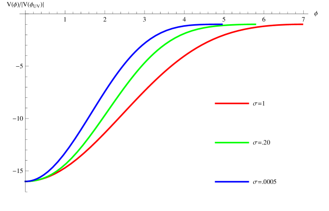
Figure 9: A parametric plot of $V(\phi)/|V_{\textrm{\tiny UV}}|$ versus $\phi$ for eq. (158) with various values of parameter $\sigma$. The other parameters in the potential are set to $L=.40$, $R=.55$ and $\gamma=.825$, as well as setting $d=4$.

Now let us consider the conformal factor given in eq. (94). Using the same equations as before, we now find

$${d\phi\over dr} \,=\, {2\sqrt{\gamma(d-1)}\over R}\,{\sqrt{1+\sigma\cosh(2r/R)}\over\sigma+\cosh(2r/R)}$$ (158)

$$V(r) \,=\, {2\gamma(d-1)\over R^{2}}\,{1+\sigma\cosh(2r/R)\over\left(\sigma+\cosh(2r/R)\right)^{2}}-d(d-1)\left(\frac{1}{L}-{\gamma\over R}\,\frac{\sinh\left({2r}/{R}\right)}{\sigma+\cosh\left({2r}/{R}\right)}\right)^{2}\,.$$

In this case, we were not able to analytically integrate $\phi^{\prime}$. However, it is straightforward to perform a numerical integration and produce a parametric plot of the potential $V$ as a function of $\phi$, as shown in figure 9. In this figure, the boundary dimension was chosen to be $d=4$ and the potential parameters are fixed as $L=.40$, $R=.55$ and $\gamma=.825$, while $\sigma$ is varied as indicated on the plot. The plot shows that qualitatively this potential has the same shape as the analytic potential found for the previous conformal factor in eq. (157) – recall that in fact, this new potential will agree with eq. (157) when $\sigma=1$. However, the new potential is becoming steeper as the parameter $\sigma$ becomes smaller. The plots only show the potential over the range relevant for the holographic RG flow, i.e., from $\phi=\phi_{\textrm{\tiny IR}}=0$ to $\phi_{\textrm{\tiny UV}}$. However, the full potential would be symmetric about both $\phi_{\textrm{\tiny IR}}$ and $\phi_{\textrm{\tiny UV}}$ and so it would be periodic with a period $\Delta\phi=2(\phi_{\textrm{\tiny UV}}-\phi_{\textrm{\tiny IR}})$. Further we note that for the parameters chosen in figure 9, the entanglement entropy undergoes a phase transition for $\sigma=.0005$ but there is no phase transition for either $\sigma=.2$ or 1.

While we were not able to produce an analytic expression for the full potential from eq. (158), it is still possible to consider a perturbative expansion around the UV critical point, i.e.,

$$V({\delta\phi})=V_{\textrm{\tiny UV}}+\frac{1}{2}\,m^{2}_{\textrm{\tiny UV}}\,{\delta\phi}^{2}+\frac{1}{24}\,\lambda_{\textrm{\tiny UV}}\,{\delta\phi}^{4}+\cdots\,,$$ (159)

where ${\delta\phi}=\phi-\phi_{\textrm{\tiny UV}}$. One can easily verify that there are no odd powers of ${\delta\phi}$ appearing in this expansion. As an example, we note that the mass parameter above would be calculated as

$$m^{2}_{\textrm{\tiny UV}}\,=\,\left.\frac{\delta^{2}V}{\delta\phi^{2}}\right|_{\phi=\phi_{\textrm{\tiny UV}}}\,=\,{1\over\phi^{\prime}}\,{d\over dr}\left({1\over\phi^{\prime}}\,{dV\over dr}\right)\bigg{|}_{r\to\infty}\,.$$ (160)

The results for the first few parameter is the expansion (159) are:

$$V_{\textrm{\tiny UV}} \,=\, -{d(d-1)\over L_{UV}^{2}}\,,\qquad\qquad m^{2}_{\textrm{\tiny UV}}\,=\,{1\over R^{2}}-{d\over L_{UV}R}$$

$$\lambda_{\textrm{\tiny UV}} \,=\, -{3d\,\sigma^{2}\,L_{UV}R+d(2-7\sigma^{2})\,L_{IR}R-8(1-2\sigma^{2})\,L_{IR}L_{UV}\over 2(d-1)\sigma^{2}\,(L_{UV}-L_{IR})R^{3}}\,,$$ (161)

where we are using the expressions in eq. (87) for $L_{UV}$ and $L_{IR}$. Of course, the value of $V_{\textrm{\tiny UV}}$ above corresponds to the expected value of the cosmological constant in the asymptotic AdS geometry. We note that the mass parameter $m^{2}_{\textrm{\tiny UV}}$ is independent of the extra parameter $\sigma$ appearing in the conformal factor (94). Hence these first two parameters precisely match those in the analogous expansion of the analytic potential in eq. (157), as is readily verified. As shown in eq. (161), the additional parameter $\sigma$ first makes its appearance the quartic coupling $\lambda_{\textrm{\tiny UV}}$. In this case, one can still verify that $\lambda_{\textrm{\tiny UV}}(\sigma=1)$ matches the analogous quartic coupling found in expanding the analytic potential (157) about $\phi=\phi_{\textrm{\tiny UV}}$. To provide some qualitative insight for this quartic coupling, we add that typically (e.g., for the parameters chosen in figure 9), $\lambda_{\textrm{\tiny UV}}$ is negative for $\sigma\sim 1$ but it becomes positive for small values of $\sigma$ (and diverges as $\sigma\to 0$).

At this point, we would like to consider the holographic interpretation of these geometries in more detail. Recall that the standard description begins with a discussion in the boundary theory where a UV critical point is perturbed by some relevant operator $\mathcal{O}$ and the latter triggers an RG flow to a new critical point in the IR. A natural assumption in this discussion is that $\mathcal{O}$ is relevant, i.e., that it has a conformal dimension $\Delta<d$. Now in the gravity description, this operator is dual to the bulk scalar $\phi$ and the conformal dimension is related to the scalar mass by the standard formula $m_{\textrm{\tiny UV}}^{2}L^{2}_{UV}=\Delta(\Delta-d)$ [63]. Inverting the latter relation yields two roots for $\Delta$, i.e.,

$$\Delta_{\pm}={d\over 2}\pm\sqrt{{d^{2}\over 4}+m_{\textrm{\tiny UV}}^{2}L^{2}_{UV}}\,,$$ (162)

where the standard choice corresponds to $\Delta=\Delta_{+}$. The scalar will have two independent solutions asymptotically [63],

$$\delta\phi\simeq e^{\Delta_{-}r/L_{UV}}\phi^{\textrm{\tiny(--)}}+e^{\Delta_{+}r/L_{UV}}\phi^{\textrm{\tiny(+)}}\,,$$ (163)

where the coefficient of the more slowly decaying solution $\phi^{\textrm{\tiny(--)}}$ corresponds to the coupling for the dual operator while $\phi^{\textrm{\tiny(+)}}$ is proportional to the expectation value $\langle\mathcal{O}\rangle$.

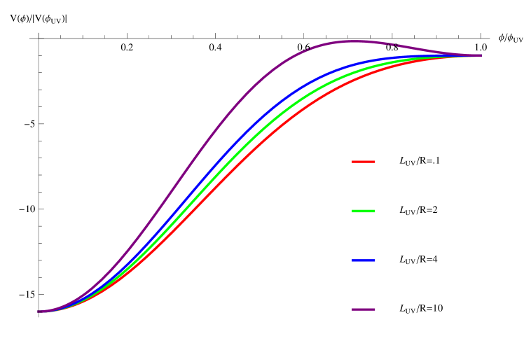
Figure 10: Plot of $V(\phi)/|V_{\textrm{\tiny UV}}|$ versus $\phi/\phi_{\textrm{\tiny UV}}$ for eq. (157) with various values of parameter $L_{UV}/R$. The parameters in the potential are chosen to fix $L_{UV}=1$ and $L_{IR}=.25$ and we set $d=4$.

Now turning to the scalar mass in eq. (161), we observe that the result can be written as $m_{\textrm{\tiny UV}}^{2}L^{2}_{UV}=\alpha(\alpha-d)$ where $\alpha=L_{UV}/R$. Further by combining eq. (95) and $\phi^{\prime}\propto\sqrt{-A^{\prime\prime}}$ from eq. (152), we see that $\alpha$ is precisely the exponent controlling the asymptotic decay of $\delta\phi$. Now there are four regimes of $\alpha$ which we consider separately: (a) $0<\alpha\leq d/2$, (b) $d/2<\alpha<(d+2)/2$, (c) $(d+2)/2<\alpha<d$ and (c) $d\leq\alpha$. In the interval (a), the holographic interpretation of the flow geometry precisely matches that described above. That is, $\alpha=\Delta_{-}$ with $\Delta_{+}=d-\Delta_{-}<d$. Hence the dual operator is relevant and leading contribution in the asymptotic decay of $\delta\phi$ reflects the fact that corresponding coupling is nonvanishing in the boundary theory. In the intervals (b) and (c), we have instead $\alpha=\Delta_{+}<d$ and hence the interpretation is that $\mathcal{O}$ is relevant but the boundary coupling for this operator vanishes. Rather holographic interpretation of the bulk solution is that $\mathcal{O}$ has a nonvanishing expectation value in the UV, which then triggers the RG flow to an new IR fixed point. Of course, this appears to be a somewhat unconventional description of RG flows. We have distinguished the interval (b) with ${d\over 2}<\alpha<{d\over 2}+1$ because in the regime, one can imagine the standard interpretation of the bulk solution still holds for the ‘alternate quantization’ of the holographic theory [65]. In the latter approach, the roles of $\phi^{\textrm{\tiny(--)}}$ and $\phi^{\textrm{\tiny(+)}}$ are reversed and the dimension of the boundary operator is given by $\Delta=\Delta_{-}$. Note that in these first three intervals (a), (b) and (c), we have $m^{2}_{\textrm{\tiny UV}}\leq 0$ and $m^{2}_{\textrm{\tiny UV}}$ reaches its minimum value at $\alpha=d/2$, where it coincides precisely with the Breitenlohner-Freedman bound [66], i.e., $m^{2}_{\textrm{\tiny UV}}L^{2}_{UV}=-d^{2}/4$. Finally in the interval (d), we have $\alpha=\Delta_{+}\geq d$ and hence in this regime, $\mathcal{O}$ is no longer a relevant operator. Rather we have an irrelevant (or marginal) operator again with a nonvanishing expectation value which triggers the flow to a new fixed point in the IR. Note that with $\alpha>d$, $m_{\textrm{\tiny UV}}^{2}>0$ and the scalar potential must have a third extremum $\phi_{3}$ between the UV and IR critical points where $V(\phi_{3})>V_{\textrm{\tiny UV}}$. This extra extremum is distinguished from the UV and IR critical points since by construction, the latter are critical points of the superpotential, whereas the new critical point satisfies $\delta V/\delta\phi|_{\phi=\phi_{3}}=0$ but $\delta W/\delta\phi|_{\phi=\phi_{3}}\neq 0$. The changing structure of the potential as $L_{UV}/R$ varies through these different regimes is illustrated in figure 10. As already noted, the interpretation of the RG flows in cases (c) and (d) in the boundary theory seems somewhat exotic. Hence one must worry that the underlying holographic model for these constructions is unphysical in some way. For example, it could be that for a consistent boundary CFT, once the dimension $\Delta$ of the operator is fixed, the quartic coupling in eq. (161) must be constrained in some way, along the lines of various bounds found in [34] or [67]. Alternatively, it could be that these background solutions are simply unstable in the corresponding parameter regime. In any event, in the main text, we focus our attention on the models in the intervals (a) and (b) for which the holographic RG flows have a conventional interpretation – see the discussion around eq. (93).

To close this section, we note that one can also consider a perturbative expansion of the scalar potential as in eq. (159) but about the IR critical point, i.e.,

$$V(\widetilde{\delta\phi})=V_{\textrm{\tiny IR}}+\frac{1}{2}\,m^{2}_{\textrm{\tiny IR}}\,\widetilde{\delta\phi}^{\,2}+\frac{1}{24}\,\lambda_{\textrm{\tiny IR}}\,\widetilde{\delta\phi}^{\,4}+\cdots\,,$$ (164)

where $\widetilde{\delta\phi}=\phi-\phi_{\textrm{\tiny IR}}$ with $\phi_{\textrm{\tiny IR}}\equiv\phi(r\to-\infty)$. As before, there are no odd powers of $\widetilde{\delta\phi}$ appearing in eq. (164). The first few parameters in this IR expansion are:

$$V_{\textrm{\tiny IR}} \,=\, -{d(d-1)\over L_{IR}^{2}}\,,\qquad\qquad m^{2}_{\textrm{\tiny IR}}\,=\,{1\over R^{2}}+{d\over L_{IR}R}$$

$$\lambda_{\textrm{\tiny IR}} \,=\, -{-d\,(2-7\sigma^{2})\,L_{UV}R-3d\,\sigma^{2}\,L_{IR}R-8(1-2\sigma^{2})\,L_{IR}L_{UV}\over 2(d-1)\sigma^{2}\,(L_{UV}-L_{IR})R^{3}}\,.$$ (165)

As in the UV expansion, we see that the parameter $\sigma$ first appears here in the quartic coupling $\lambda_{\textrm{\tiny IR}}$. Hence one can easily verify that $V_{\textrm{\tiny IR}}$ and $m^{2}_{\textrm{\tiny IR}}$ precisely match the corresponding couplings in the IR expansion of the analytic potential in eq. (157), while $\lambda_{\textrm{\tiny IR}}$ matches the quartic coupling in this expansion when $\sigma=1$. Note that $m^{2}_{\textrm{\tiny IR}}>0$ and so the dual operator is always irrelevant at the IR critical point. The behaviour of the quartic coupling is qualitatively the same as described above for $\lambda_{\textrm{\tiny IR}}$, i.e., it is typically negative for $\sigma\sim 1$ and positive for $\sigma\sim 0$.

References

- [1] A. B. Zamolodchikov, “Irreversibility of the Flux of the Renormalization Group in a 2D Field Theory,” JETP Lett. 43, 730 (1986).
-
[2]
H. Casini and M. Huerta,
“A finite entanglement entropy and the c-theorem,”
Phys. Lett. B 600, 142 (2004)
[arXiv:hep-th/0405111];
H. Casini and M. Huerta, “A c-theorem for the entanglement entropy,” J. Phys. A 40, 7031 (2007) [arXiv:cond-mat/0610375]. - [3] P. Calabrese and J. L. Cardy, “Entanglement entropy and quantum field theory,” J. Stat. Mech. 0406, P002 (2004) [arXiv:hep-th/0405152].
-
[4]
P. Calabrese and J. L. Cardy, “Entanglement entropy and quantum field
theory: A non-technical introduction,”
Int. J. Quant. Inf. 4, 429 (2006)
[arXiv:quant-ph/0505193];
P. Calabrese and J. Cardy, “Entanglement entropy and conformal field theory,” J. Phys. A 42 (2009) 504005 [arXiv:0905.4013 [cond-mat.stat-mech]]. - [5] J. L. Cardy, “Is There a c Theorem in Four-Dimensions?,” Phys. Lett. B 215, 749 (1988).
- [6] H. Osborn, “Derivation of a Four-Dimensional c-theorem,” Phys. Lett. B 222, 97 (1989).
- [7] D. Anselmi, D.Z. Freedman, M.T. Grisaru and A.A. Johansen, “Nonperturbative formulas for central functions of supersymmetric gauge theories,” Nucl. Phys. B 526, 543 (1998) [arXiv:hep-th/9708042].
- [8] D. Anselmi, J. Erlich, D.Z. Freedman and A.A. Johansen, “Positivity constraints on anomalies in supersymmetric gauge theories,” Phys. Rev. D 57, 7570 (1998) [arXiv:hep-th/9711035].
-
[9]
K. A. Intriligator and B. Wecht,
“The exact superconformal R-symmetry maximizes a,”
Nucl. Phys. B 667, 183 (2003)
[arXiv:hep-th/0304128];
E. Barnes, K. A. Intriligator, B. Wecht and J. Wright, “Evidence for the strongest version of the 4d a-theorem, via a-maximization along RG flows,” Nucl. Phys. B 702, 131 (2004) [arXiv:hep-th/0408156]. - [10] D. Gaiotto, N. Seiberg and Y. Tachikawa, “Comments on scaling limits of 4d N=2 theories,” arXiv:1011.4568 [hep-th].
- [11] A.D. Shapere and Y. Tachikawa, “A counterexample to the ’a-theorem’,” JHEP 0812, 020 (2008) [arXiv:0809.3238 [hep-th]].
-
[12]
Z. Komargodski and A. Schwimmer,
“On Renormalization Group Flows in Four Dimensions,”
arXiv:1107.3987 [hep-th];
Z. Komargodski, “The Constraints of Conformal Symmetry on RG Flows,” arXiv:1112.4538 [hep-th]. - [13] A. Schwimmer and S. Theisen, “Spontaneous Breaking of Conformal Invariance and Trace Anomaly Matching,” Nucl. Phys. B 847, 590 (2011) [arXiv:1011.0696 [hep-th]].
- [14] A. Adams, N. Arkani-Hamed, S. Dubovsky, A. Nicolis and R. Rattazzi, “Causality, analyticity and an IR obstruction to UV completion,” JHEP 0610 (2006) 014 [arXiv:hep-th/0602178].
-
[15]
D. Dorigoni and V. S. Rychkov,
“Scale Invariance + Unitarity =¿ Conformal Invariance?,”
arXiv:0910.1087 [hep-th];
S. El-Showk, Y. Nakayama and S. Rychkov, “What Maxwell Theory in D¡¿4 teaches us about scale and conformal invariance,” Nucl. Phys. B 848, 578 (2011) [arXiv:1101.5385 [hep-th]];
R. Jackiw and S. Y. Pi, “Tutorial on Scale and Conformal Symmetries in Diverse Dimensions,” J. Phys. A 44, 223001 (2011) [arXiv:1101.4886 [math-ph]];
I. Antoniadis and M. Buican, “On R-symmetric Fixed Points and Superconformality,” Phys. Rev. D 83, 105011 (2011) [arXiv:1102.2294 [hep-th]];
M. Buican, “A Conjectured Bound on Accidental Symmetries,” arXiv:1109.3279 [hep-th];
Y. Nakayama, “Comments on scale invariant but non-conformal supersymmetric field theories,” arXiv:1109.5883 [hep-th];
Y. Nakayama, “On -conjecture in a-theorem,” arXiv:1110.2586 [hep-th];
T. L. Curtright, X. Jin and C. K. Zachos, “RG flows, cycles, and c-theorem folklore,” arXiv:1111.2649 [hep-th]. -
[16]
J. F. Fortin, B. Grinstein and A. Stergiou,
“Scale without Conformal Invariance: An Example,”
Phys. Lett. B 704, 74 (2011)
[arXiv:1106.2540 [hep-th]];
J. F. Fortin, B. Grinstein and A. Stergiou, “Scale without Conformal Invariance: Theoretical Foundations,” arXiv:1107.3840 [hep-th]. - [17] J. Polchinski, “Scale and Conformal Invariance in Quantum Field Theory,” Nucl. Phys. B 303, 226 (1988).
- [18] D.Z. Freedman, S.S. Gubser, K. Pilch and N.P. Warner, “Renormalization group flows from holography supersymmetry and a c-theorem,” Adv. Theor. Math. Phys. 3, 363 (1999) [arXiv:hep-th/9904017].
-
[19]
L. Girardello, M. Petrini, M. Porrati and
A. Zaffaroni,
“Novel local CFT and exact results on perturbations of N = 4 super
Yang-Mills from AdS dynamics,”
JHEP 9812, 022 (1998) [arXiv:hep-th/9810126];
L. Girardello, M. Petrini, M. Porrati and A. Zaffaroni, “The supergravity dual of N = 1 super Yang-Mills theory,” Nucl. Phys. B 569, 451 (2000) [arXiv:hep-th/9909047]. -
[20]
R. C. Myers and A. Sinha,
“Seeing a c-theorem with holography,”
Phys. Rev. D 82, 046006 (2010)
[arXiv:1006.1263 [hep-th]];
R. C. Myers and A. Sinha, “Holographic c-theorems in arbitrary dimensions,” JHEP 1101, 125 (2011) [arXiv:1011.5819 [hep-th]]. - [21] H. Casini, M. Huerta and R. C. Myers, “Towards a derivation of holographic entanglement entropy,” JHEP 1105, 036 (2011) [arXiv:1102.0440 [hep-th]].
-
[22]
D. L. Jafferis,
“The Exact Superconformal R-Symmetry Extremizes Z,”
arXiv:1012.3210 [hep-th];
D. L. Jafferis, I. R. Klebanov, S. S. Pufu and B. R. Safdi, “Towards the F-Theorem: N=2 Field Theories on the Three-Sphere,” JHEP 1106, 102 (2011) [arXiv:1103.1181 [hep-th]];
I. R. Klebanov, S. S. Pufu and B. R. Safdi, “F-Theorem without Supersymmetry,” arXiv:1105.4598 [hep-th];
I. R. Klebanov, S. S. Pufu, S. Sachdev and B. R. Safdi, “Entanglement Entropy of 3-d Conformal Gauge Theories with Many Flavors,” arXiv:1112.5342 [hep-th]. - [23] J. de Boer, M. Kulaxizi and A. Parnachev, “Holographic Entanglement Entropy in Lovelock Gravities,” JHEP 1107, 109 (2011) [arXiv:1101.5781 [hep-th]].
- [24] L. Y. Hung, R. C. Myers and M. Smolkin, “Some Calculable Contributions to Holographic Entanglement Entropy,” JHEP 1108, 039 (2011) [arXiv:1105.6055 [hep-th]].
- [25] T. Albash and C. V. Johnson, “Holographic Entanglement Entropy and Renormalization Group Flow,” arXiv:1110.1074 [hep-th].
- [26] H. Liu and M. Mezei, “A refinement of entanglement entropy and the number of degrees of freedom,” arXiv:1202.2070 [hep-th].
-
[27]
See, for example:
S.W. Hawking and G.F.R. Ellis, The Large scale structure of space-time, (Cambridge University Press, Cambridge, 1973). -
[28]
See, for example:
M. J. Duff, “Observations On Conformal Anomalies,” Nucl. Phys. B 125, 334 (1977);
M. J. Duff, “Twenty years of the Weyl anomaly,” Class. Quant. Grav. 11, 1387 (1994) [arXiv:hep-th/9308075]. - [29] S. Deser and A. Schwimmer, “Geometric classification of conformal anomalies in arbitrary dimensions,” Phys. Lett. B 309, 279 (1993) [arXiv:hep-th/9302047].
-
[30]
C. Fefferman and C. R. Graham, “Conformal Invariants,” in Elie Cartan et les
Mathématiques d’aujourd hui (Astérisque, 1985) 95;
C. Fefferman and C. R. Graham, “The Ambient Metric,” arXiv:0710.0919 [math.DG]. -
[31]
M. Henningson and K. Skenderis,
“The holographic Weyl anomaly,” JHEP 9807, 023 (1998)
[arXiv:hep-th/9806087];
M. Henningson and K. Skenderis, “Holography and the Weyl anomaly,” Fortsch. Phys. 48, 125 (2000) [arXiv:hep-th/9812032]. -
[32]
S. Nojiri and S.D. Odintsov,
“On the conformal anomaly from higher derivative gravity in AdS/CFT
correspondence,”
Int. J. Mod. Phys. A 15, 413 (2000)
[arXiv:hep-th/9903033];
M. Blau, K.S. Narain and E. Gava, “On subleading contributions to the AdS/CFT trace anomaly,” JHEP 9909, 018 (1999) [arXiv:hep-th/9904179]. -
[33]
D. Lovelock, “The Einstein tensor and its generalizations,”
J. Math. Phys. 12, 498 (1971);
D. Lovelock, “Divergence-free tensorial concomitants,” Aequationes Math. 4, 127 (1970). -
[34]
M. Brigante, H. Liu, R. C. Myers, S. Shenker and
S. Yaida, “Viscosity Bound Violation in Higher Derivative Gravity,”
Phys. Rev. D 77 (2008) 126006
[arXiv:htp-th/0712.0805];
M. Brigante, H. Liu, R. C. Myers, S. Shenker and S. Yaida, “The Viscosity Bound and Causality Violation,” Phys. Rev. Lett. 100, 191601 (2008) [arXiv:0802.3318 [hep-th]];
A. Buchel and R. C. Myers, “Causality of Holographic Hydrodynamics,” JHEP 0908, 016 (2009) [arXiv:0906.2922 [hep-th]];
D. M. Hofman, “Higher Derivative Gravity, Causality and Positivity of Energy in a UV complete QFT,” Nucl. Phys. B 823, 174 (2009) [arXiv:0907.1625 [hep-th]];
X. H. Ge and S. J. Sin, “Shear viscosity, instability and the upper bound of the Gauss-Bonnet coupling constant,” JHEP 0905, 051 (2009) [arXiv:0903.2527 [hep-th]];
R. G. Cai, Z. Y. Nie and Y. W. Sun, “Shear Viscosity from Effective Couplings of Gravitons,” Phys. Rev. D 78, 126007 (2008) [arXiv:0811.1665 [hep-th]];
R. G. Cai, Z. Y. Nie, N. Ohta and Y. W. Sun, “Shear Viscosity from Gauss-Bonnet Gravity with a Dilaton Coupling,” Phys. Rev. D 79, 066004 (2009) [arXiv:0901.1421 [hep-th]];
J. de Boer, M. Kulaxizi and A. Parnachev, “, Gauss-Bonnet Gravity, and Viscosity Bound,” JHEP 1003, 087 (2010) [arXiv:0910.5347 [hep-th]];
X. O. Camanho and J. D. Edelstein, “Causality constraints in AdS/CFT from conformal collider physics and Gauss-Bonnet gravity,” arXiv:0911.3160 [hep-th]. - [35] D. G. Boulware and S. Deser, “String Generated Gravity Models,” Phys. Rev. Lett. 55 (1985) 2656.
-
[36]
R. C. Myers and B. Robinson,
“Black Holes in Quasi-topological Gravity,”
JHEP 1008, 067 (2010)
[arXiv:1003.5357 [gr-qc]];
R. C. Myers, M. F. Paulos and A. Sinha, “Holographic studies of quasi-topological gravity,” JHEP 1008, 035 (2010) [arXiv:1004.2055 [hep-th]]. - [37] A. Buchel, J. Escobedo, R. C. Myers, M. F. Paulos, A. Sinha and M. Smolkin, “Holographic GB gravity in arbitrary dimensions,” JHEP 1003 (2010) 111 [arXiv:0911.4257 [hep-th]].
- [38] L. Y. Hung, R. C. Myers, M. Smolkin and A. Yale, “Holographic Calculations of Renyi Entropy,” arXiv:1110.1084 [hep-th].
-
[39]
C. Imbimbo, A. Schwimmer, S. Theisen and S. Yankielowicz,
“Diffeomorphisms and holographic anomalies,”
Class. Quant. Grav. 17, 1129 (2000)
[arXiv:hep-th/9910267];
A. Schwimmer and S. Theisen, “Entanglement Entropy, Trace Anomalies and Holography,” Nucl. Phys. B 801, 1 (2008) [arXiv:0802.1017 [hep-th]]. - [40] A. Sinha, “On higher derivative gravity, -theorems and cosmology,” Class. Quant. Grav. 28, 085002 (2011) [arXiv:1008.4315 [hep-th]].
- [41] J. T. Liu, W. Sabra and Z. Zhao, “Holographic c-theorems and higher derivative gravity,” arXiv:1012.3382 [hep-th].
- [42] M. F. Paulos, “Holographic phase space: -functions and black holes as renormalization group flows,” JHEP 1105, 043 (2011) [arXiv:1101.5993 [hep-th]].
- [43] A. Allais, “Double-trace deformations, holography and the c-conjecture,” JHEP 1011, 040 (2010) [arXiv:1007.2047 [hep-th]].
-
[44]
R. V. Buniy, S. D. H. Hsu and B. M. Murray,
“The null energy condition and instability,”
Phys. Rev. D 74, 063518 (2006) [arXiv:hep-th/0606091];
S. Dubovsky, T. Gregoire, A. Nicolis and R. Rattazzi, “Null energy condition and superluminal propagation,” JHEP 0603, 025 (2006) [arXiv:hep-th/0512260]. - [45] S. Ryu and T. Takayanagi, “Holographic derivation of entanglement entropy from AdS/CFT,” Phys. Rev. Lett. 96, 181602 (2006) [arXiv:hep-th/0603001].
- [46] S. Ryu and T. Takayanagi, “Aspects of holographic entanglement entropy,” JHEP 0608, 045 (2006) [arXiv:hep-th/0605073].
- [47] M. Headrick, “Entanglement Renyi entropies in holographic theories,” Phys. Rev. D 82, 126010 (2010) [arXiv:1006.0047 [hep-th]].
- [48] D. V. Fursaev, “Proof of the holographic formula for entanglement entropy,” JHEP 0609, 018 (2006) [arXiv:hep-th/0606184].
- [49] L. Y. Hung, R. C. Myers and M. Smolkin, “On Holographic Entanglement Entropy and Higher Curvature Gravity,” JHEP 1104, 025 (2011) [arXiv:1101.5813 [hep-th]].
- [50] T. Jacobson, R. C. Myers, “Black hole entropy and higher curvature interactions,” Phys. Rev. Lett. 70, 3684-3687 (1993). [hep-th/9305016].
-
[51]
R. M. Wald, “Black hole entropy is the
Noether charge,”
Phys. Rev. D 48, 3427 (1993)
[arXiv:gr-qc/9307038];
V. Iyer and R. M. Wald, “Some properties of Noether charge and a proposal for dynamical black hole entropy,” Phys. Rev. D 50, 846 (1994) [arXiv:gr-qc/9403028];
T. Jacobson, G. Kang and R. C. Myers, “On Black Hole Entropy,” Phys. Rev. D 49, 6587 (1994) [arXiv:gr-qc/9312023]. -
[52]
See, for example:
E. Witten, “Anti-de Sitter space, thermal phase transition, and confinement in gauge theories,” Adv. Theor. Math. Phys. 2, 505 (1998) [arXiv:hep-th/9803131];
A. Chamblin, R. Emparan, C. V. Johnson and R. C. Myers, “Charged AdS black holes and catastrophic holography,” Phys. Rev. D 60, 064018 (1999) [arXiv:hep-th/9902170];
D. Mateos, R. C. Myers and R. M. Thomson, “Holographic phase transitions with fundamental matter,” Phys. Rev. Lett. 97, 091601 (2006) [arXiv:hep-th/0605046]. -
[53]
A. Sinha,
“On the new massive gravity and AdS/CFT,”
JHEP 1006, 061 (2010)
[arXiv:1003.0683 [hep-th]];
M. F. Paulos, “New massive gravity extended with an arbitrary number of curvature corrections,” Phys. Rev. D 82, 084042 (2010) [arXiv:1005.1646 [hep-th]];
I. Gullu, T. C. Sisman and B. Tekin, “c-functions in the Born-Infeld extended New Massive Gravity,” Phys. Rev. D 82, 024032 (2010) [arXiv:1005.3214 [hep-th]]. - [54] T. Hirata and T. Takayanagi, “AdS/CFT and strong subadditivity of entanglement entropy,” JHEP 0702, 042 (2007) [hep-th/0608213].
- [55] I. R. Klebanov, D. Kutasov and A. Murugan, “Entanglement as a probe of confinement,” Nucl. Phys. B 796, 274 (2008) [arXiv:0709.2140 [hep-th]].
- [56] A. Pakman and A. Parnachev, “Topological Entanglement Entropy and Holography,” JHEP 0807, 097 (2008) [arXiv:0805.1891 [hep-th]].
- [57] T. Albash and C. V. Johnson, “Holographic Studies of Entanglement Entropy in Superconductors,” arXiv:1202.2605 [hep-th].
- [58] T. Albash and C. V. Johnson, “Evolution of Holographic Entanglement Entropy after Thermal and Electromagnetic Quenches,” New J. Phys. 13, 045017 (2011) [arXiv:1008.3027 [hep-th]].
- [59] K. Skenderis and P. K. Townsend, “Gravitational stability and renormalization group flow,” Phys. Lett. B 468, 46 (1999) [arXiv:hep-th/9909070].
- [60] O. DeWolfe, D. Z. Freedman, S. S. Gubser and A. Karch, “Modeling the fifth-dimension with scalars and gravity,” Phys. Rev. D 62, 046008 (2000) [arXiv:hep-th/9909134].
- [61] I. Low, A. Zee, “Naked singularity and Gauss-Bonnet term in brane world scenarios,” Nucl. Phys. B585, 395-404 (2000). [hep-th/0004124].
- [62] U. d. .Camara and G. M. Sotkov, “New Massive Gravity Domain Walls,” Phys. Lett. B 694, 94 (2010) [arXiv:1008.2553 [hep-th]].
- [63] O. Aharony, S. S. Gubser, J. M. Maldacena, H. Ooguri and Y. Oz, “Large N field theories, string theory and gravity,” Phys. Rept. 323, 183 (2000) [arXiv:hep-th/9905111].
- [64] E. Gava, P. Karndumri and K. S. N. Narain, “ vacua and RG flows in three dimensional gauged supergravities,” JHEP 1004, 117 (2010) [arXiv:1002.3760 [hep-th]].
- [65] I. R. Klebanov and E. Witten, “AdS/CFT correspondence and symmetry breaking,” Nucl. Phys. B 556, 89 (1999) [arXiv:hep-th/9905104].
-
[66]
P. Breitenlohner and D. Z. Freedman,
“Positive Energy In Anti-De Sitter Backgrounds And Gauged Extended
Supergravity,”
Phys. Lett. B 115, 197 (1982);
P. Breitenlohner and D. Z. Freedman, “Stability In Gauged Extended Supergravity,” Annals Phys. 144, 249 (1982);
L. Mezincescu and P. K. Townsend, “Stability At A Local Maximum In Higher Dimensional Anti-De Sitter Space And Applications To Supergravity,” Annals Phys. 160, 406 (1985). -
[67]
D. M. Hofman and J. Maldacena,
“Conformal collider physics: Energy and charge correlations,”
JHEP 0805, 012 (2008)
[arXiv:0803.1467 [hep-th]];
R. Rattazzi, V. S. Rychkov, E. Tonni and A. Vichi, “Bounding scalar operator dimensions in 4D CFT,” JHEP 0812, 031 (2008) [arXiv:0807.0004 [hep-th]];
S. Hellerman, “A Universal Inequality for CFT and Quantum Gravity,” JHEP 1108, 130 (2011) [arXiv:0902.2790 [hep-th]];
V. S. Rychkov and A. Vichi, “Universal Constraints on Conformal Operator Dimensions,” Phys. Rev. D 80, 045006 (2009) [arXiv:0905.2211 [hep-th]];
D. Poland and D. Simmons-Duffin, “Bounds on 4D Conformal and Superconformal Field Theories,” JHEP 1105, 017 (2011) [arXiv:1009.2087 [hep-th]].