Faraday waves in binary non-miscible Bose-Einstein condensates

Abstract

We show by extensive numerical simulations and analytical variational calculations that elongated binary non-miscible Bose-Einstein condensates subject to periodic modulations of the radial confinement exhibit a Faraday instability similar to that seen in one-component condensates. Considering the hyperfine states of ⁸⁷Rb condensates, we show that there are two experimentally relevant stationary state configurations: the one in which the components form a dark-bright symbiotic pair (the ground state of the system), and the one in which the components are segregated (first excited state). For each of these two configurations, we show numerically that far from resonances the Faraday waves excited in the two components are of similar periods, emerge simultaneously, and do not impact the dynamics of the bulk of the condensate. We derive analytically the period of the Faraday waves using a variational treatment of the coupled Gross-Pitaevskii equations combined with a Mathieu-type analysis for the selection mechanism of the excited waves. Finally, we show that for a modulation frequency close to twice that of the radial trapping, the emergent surface waves fade out in favor of a forceful collective mode that turns the two condensate components miscible.

I Introduction

The excitation of surface waves through parametric resonances is one of the oldest pattern-forming processes that goes back to Ernst Chladni’s “beautiful series of forms assumed by sand, fillings, or other grains when lying upon vibrating plates” that “are so striking as to be recalled to the minds of those who have seen them by the slightest reference”, Hans Christian Ørsted’s experiments with lycopodium light powders, and Michael Faraday’s “crispations” seen in “fluids in contact with vibrating surfaces” Faraday1831 . The prototypical example of parametric wave excitation is that of a shallow disc of a liquid rigidly oscillated in the vertical direction. In this setting the acceleration periodically modulates the effective gravity and for drives of sufficiently large amplitudes a surface wave instability occurs with frequency one half that of the drive CrossHohenberg . Such surface waves are termed Faraday waves, and the corresponding pattern-forming phenomenon has been seen in numerous Newtonian and non-Newtonian fluids, colloidal suspensions, ferromagnetic bodies, and, more recently, in superfluids.

After a series of inceptive studies on extended parametric resonances in confined superfluids PR-orig ; StaliunasOne-1 ; StaliunasTwo-1 ; paramresOLorig ; paramresOL ; ModugnioPF , the experimental observation of Faraday waves in ⁴He cells FaradayHe and ⁸⁷Rb cigar-shaped Bose-Einstein condensates (BECs) EngelsFaraday catalyzed the interest in the nonlinear dynamics of parametrically-driven ultracold gases PanosBook . In addition to the ever-present collective oscillation modes of BECs hu1 , their parametric driving can generate soundlike density waves, which are analogous to Faraday surface waves. BEC systems also exhibit resonances, and when the driving frequency is close to one of them, forceful resonant waves can develop, eventually taking over the dynamics of the system. Furthermore, inherent nonlinearity of such systems brings about a diverse set of related dynamical phenomena and leads to their complex interplay.

Surveying the recent literature for bosonic systems one notices the theoretical investigations into the soliton management in periodic systems MalomedBook ; hadzievski , the emergence and suppression of Faraday patterns AlexPanos ; FaradayTwoComp ; PhysACArina ; santos ; capuzzidoi , the parametric excitation of resonances hu2 and “scars” in BECs katz , spatially and temporally driven atomic interactions in optical lattices gaul1 ; sekh , quantized vortices induced by spatio-temporally modulated interaction wang , stability and decay of Bloch oscillations in the presence of time-dependent nonlinearity gaul2 ; gaul3 , and, quite interestingly, the removal of excitations in BECs subject to time-dependent periodic potentials StaliunasSuppresion . On a related topic, the formation of density waves has been predicted for expanding condensates densitymodulationsSalasnich ; Imambekov and the spontaneous formation of density waves has been recently reported for antiferromagnetic BECs SpontPattFormBEC . Faraday waves have been analyzed in detail also in superfluid fermionic gases Capuzzi ; Tang and it has been shown that the collective modes of 1D fermionic systems can be amplified by parametric resonances to the extent of observing a clear spin-charge separation graf .

Parametric resonances in BECs are usually achieved through periodic modulation of the frequency of the trapping potential, as is the case in Ref. EngelsFaraday , but the recent experiments on the collective modes of a trapped ⁷Li BEC through periodic modulation of the scattering length Pollack have opened a new direction for both experimental and theoretical Ivana investigations. Simultaneous modulations of the strength of the confining potential and of the scattering length, in particular, are largely unexplored. They can give rise to new recipes for pattern formation and, possibly, to new types of patterns.

In this paper we study the excitation of waves through periodic modulations of the radial confinement of binary non-miscible BECs and show that these condensates exhibit a Faraday instability similar to that seen in one-component systems. Considering the hyperfine states of realistic ⁸⁷Rb condensates which can be readily produced Jovana , such as $\left|1,-1\right\rangle$, $\left|2,0\right\rangle$ and $\left|1,-1\right\rangle$, $\left|2,1\right\rangle$ pairs, we show that there are two distinct experimentally relevant stationary configurations: one where the components form a dark-bright symbiotic pair, which is the ground state of the system, and one where the components are segregated, which is the first excited state of the system. Far from resonances we show numerically for each configuration that the excited waves are of similar periods and emerge simultaneously, and analytically find the dispersion relation using a variational treatment in conjunction with a Mathieu-type analysis. Finally, the resonant excitation of collective modes is analyzed in detail.

The rest of the paper is structured as follows. In Sec. II we describe the numerical treatment of the coupled Gross-Pitaevskii equations (GPEs) that describe the $T=0$ dynamics of the condensate and introduce the two types of stationary configurations, while in Sec. III we derive the corresponding variational equations and the associated dispersion relations. In Sec. IV we present our numerical and analytical results for realistic ⁸⁷Rb condensates, along with suggestions for future experiments. The last section contains conclusions and outlook.

II Stationary states

The dynamics of binary condensates at $T=0$ is governed by the time-dependent version of the coupled GPEs, which read Book

$$i\frac{\partial\psi_{j}}{\partial t} = -\frac{1}{2}\Delta\psi_{j}+V({\bf r},t)\psi_{j}+N_{j}U_{j}\left|\psi_{j}\right|^{2}\psi_{j}$$ (1)

$$+N_{3-j}\tilde{U}\left|\psi_{3-j}\right|^{2}\psi_{j},$$

where $j\in\{1,2\}$, $N_{j}$ is the fixed number of atoms in each component, $U_{j}=4\pi a_{j}$, $\tilde{U}=4\pi\tilde{a}$, with $a_{j}$ being the intra-component scattering lengths, while $\tilde{a}$ is the inter-component scattering length. Here we use numerical values similar to the experimental ones from Refs. scattlengths ; DarkBrightPhysLettA ; segprl ,

$$a_{1}=100.4\,a_{0}\,,\quad a_{2}=98.98\,a_{0}\,,\quad\tilde{a}=a_{1}\,,$$ (2)

where $a_{0}$ is the Bohr radius. Small variations in scattering lengths yield similar results, but we have chosen these particular values since they correspond to a clearly non-miscible configuration at the mean-field level, thereby emphasizing the forcefulness of the miscibility transition, which represents one of our main motivations, as we will see in Sec. IV. For simplicity, we use natural units $\hbar=m=1$ throughout the paper, and component normalization

$$\int d{\bf r}\left|\psi_{j}({\bf r},t)\right|^{2}=1\,.$$ (3)

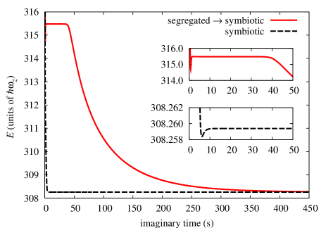
Figure 1: (Color online) Typical imaginary-time propagation of the total energy for a two-component condensate system with $N_{1}=2.5\cdot 10^{5}$ atoms in the state A and $N_{2}=1.25\cdot 10^{5}$ in the state B, $\Omega_{\rho}=160\times 2\pi$ Hz, $\Omega_{z}=7\times 2\pi$ Hz. The dashed black curve corresponds to the evolution from initial wave functions set to two identical Gaussians, which immediately yields the ground state, while the full red curve corresponds to evolution from the initial wave functions set to two well-separated Gaussians, yielding the first excited state of the system, which eventually decays to the ground state.

The stationary states of binary Bose-Einstein condensates are obtained by solving the time-independent version of Eqs. (1), in which terms with time derivatives of wave functions are replaced by the terms containing chemical potentials $\mu_{j}$ of components,

$$-\frac{1}{2}\Delta\psi_{j}+V({\bf r},t)\psi_{j}+N_{j}U_{j}\left|\psi_{j}\right|^{2}\psi_{j}$$

$$+N_{3-j}\tilde{U}\left|\psi_{3-j}\right|^{2}\psi_{j} = \mu_{j}\psi_{j}.$$ (4)

In this paper we consider the two hyperfine states of ⁸⁷Rb (hereafter referred to as states A and B) in an external potential of the form

$$V({\bf r},t)=\frac{1}{2}\Omega_{\rho}^{2}(t)\rho^{2}+\frac{1}{2}\Omega_{z}^{2}z^{2},$$ (5)

where $\rho^{2}=x^{2}+y^{2}$, such that the system is cylindrically-symmetric, i.e. $\psi_{j}({\bf r},t)\equiv\psi_{j}(\rho,z,t)$, and GPEs are effectively two-dimensional. We also assume that the system is highly elongated and strongly confined in the radial direction, $\Omega_{\rho}(t)\gg\Omega_{z}$. The above time-dependent system of GPEs (1), as well as its time-independent counterpart Eq. (4), can be solved numerically using various approaches pla-manybody ; balazpre ; diag1 ; diag2 ; becpla . Here we choose the efficient split-step Crank-Nicolson approach developed by Adhikari and Muruganandam in Ref. AdhikariCode . We have implemented this algorithm in the C programming language, and use it for all numerical simulations presented here.

Binary condensates exhibit a wide range of interesting and experimentally relevant configurations, which go from the one-dimensional soliton pairs tabulated in Ref. 2CompSolPairs , to the more exotic two-dimensional vortex-lattices 2CompVorLatt , and vortex-bright-soliton structures 2CompVortexBrightSol . From the mean-field theory it follows that binary condensates are miscible if the condition $\tilde{U}<\sqrt{U_{1}U_{2}}$ is satisfied AoChui . For the values from Eq. (2) this condition is not satisfied, and the system is non-miscible scattlengths .

The stationary states are computed numerically by imaginary-time propagation until we achieve the convergence of wave functions and physical quantities of the system, chemical potentials and mean-square radii of components, and the total system energy. Fig. 1 illustrates the results obtained using this approach for different initial conditions. It shows total energy of the system as a function of the imaginary time. Using the various initial conditions, we were able to numerically calculate two relevant stationary configurations: the one in which the components form a dark-bright symbiotic pair (ground state), and the one in which the components are spatially well segregated. From Fig. 1 we can see that the segregated state is a first excited state of the system, as it decays to the ground state after sufficiently long imaginary-time propagation.

The first type of stationary solutions supported by the GPEs, the ground state, consists of a symmetric, Thomas-Fermi-type density profile with a hole in the center in one component, and a well-localized density peak positioned in the center of the trap in the other component. Fig. 2 shows typical longitudinal density profiles

$$n_{j}(z)=\int_{0}^{\infty}d\rho\ 2\pi\rho\left|\psi_{j}(\rho,z)\right|^{2}$$ (6)

of the two components for the ground state, obtained through the imaginary-time propagation, starting from the two identical Gaussian initial states.

We note the apparent similarity of the obtained dark-bright symbiotic solutions and the dark-bright soliton molecules, known to exist in homogenous systems. These soliton molecules were originally predicted in a nonlinear optics setting DBThOne ; DBThTwo and were first observed in photorefractive crystals DBSolitonsOptics . Following their exposure to the BEC community PredictionDBOrigTheor , they were observed experimentally using the ⁸⁷Rb condensates DBSolitonFirstExp , and were subsequently addressed theoretically in Refs. NistazakisDB ; DarkBrightPhysLettA ; PerezGarciaDBSoliton . In homogeneous condensates the dark component effectively acts as a trapping potential for the bright component through the nonlinear interaction, and this mechanism is well preserved in inhomogeneous systems, albeit the dark component is cut-off away from the center of the trap and the bright component tends to be more narrow due to the additional confinement by the trap. However, symbiotic solutions from Fig. 2 do not represent inhomogeneous counterparts of soliton molecules, since they are purely real, and the first component does not exhibit a jump of $\pi$ in the phase between its left and right part.

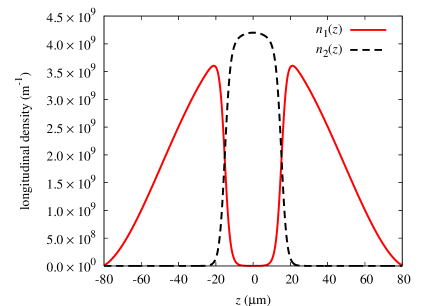
Figure 2: (Color online) Typical longitudinal density profiles for a condensate in the ground state (dark-bright symbiotic pair). The parameters are the same as in Fig. 1, the full red curve shows the density profile for atoms in the state A, the dashed black line for atoms in the state B.

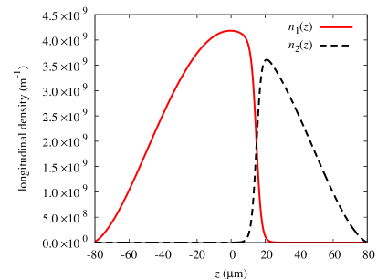
Figure 3: (Color online) Typical longitudinal density profiles for a condensate in the first excited state (segregated state). The parameters are the same as in Fig. 1, the full red curve shows the density profile for atoms in the state A, the dashed black line for atoms in the state B.

The second type of stationary solutions supported by the GPEs, the first excited state, is presented in Fig. 3. It consists of two opposing, asymmetric Thomas-Fermi-type density profiles, with the negligible overlap. This segregation of the components stems from the repulsive character of the interaction and the non-miscible nature of the considered binary condensate. Naturally, there exist a large number of further excited states of the system that can be calculated numerically as well, but we focus only on the two relevant states, shown in Figs. 2 and 3.

Experimentally, such states can readily be realized using current technology. While our analysis considers elongated traps approaching a one-dimensional limit, we note that the state in Fig. 2 has already been observed in three-dimensional traps where a magnetically trapped BEC of ⁸⁷Rb atoms was prepared in a mixture of the $\left|1,-1\right\rangle$ and $\left|2,1\right\rangle$ hyperfine states and was observed to assume a ball-shell structure cornell ; hall . By introducing differential trap shifts for the two components as in Ref. cornell , the segregated state in Fig. 3 can readily be generated as well. Alternatively, optical traps can be employed to confine atoms in a state independent way, and an additional magnetic gradient can be used to separate components of a mixture. Using a miscible mixture, this phase separation in an optical trap has been generated e.g. in Ref. segprl and can also be extended to optical lattice systems ketterle . Using a microwave sweep in a high-bias magnetic field, the miscible mixture in the latter experiments can be converted into an immiscible mixture by changing the hyperfine state of one of the components.

At the end, let us also note that the stationary character of the two numerically calculated states presented here was cross-checked by performing a real-time propagation for long time intervals (much longer than those considered in the rest of the paper). While in the imaginary-time propagation the first excited state eventually decays to the ground state, when real-time propagation is performed both stationary states are found to be stable for all practical purposes.

III Variational treatment

In this section we develop variational analytic approach suitable for study of the emergence and characterization of Faraday patterns in non-miscible binary condensates, induced by harmonic modulation of the radial trapping frequency. For each of the two stationary states calculated in Sec. II, we propose a suitable variational ansatz for component wave functions, approximately solve the ensuing equations, and analytically derive expressions for periods of Faraday waves induced far from resonances. The obtained analytical results are compared with the numerical results in Sec. IV.

III.1 Symbiotic pair state

To construct a suitable variational ansatz for component wave functions in the case of the symbiotic pair state, we consider an equivalent one-component scenario, in which the bright state $\psi_{2}$ evolves in the combined effective field created by the dark state $\psi_{1}$ and by the trapping potential. To further simplify the problem, in this subsection we will also assume that the values of three scattering lengths from Eq. (2) are equal, namely $a_{1}=a_{2}=\tilde{a}\equiv a=100.4\,a_{0}$, or $U_{1}=U_{2}=\tilde{U}\equiv U$, which is justified since the values measured experimentally are quite close scattlengths .

In this setting, the effective one-component Lagrangian density for the bright state $\psi_{2}$ is given by

$${\cal L}_{2}(\rho,z,t) = \frac{i}{2}\left(\psi_{2}\frac{\partial\psi_{2}^{*}}{\partial t}-\psi_{2}^{*}\frac{\partial\psi_{2}}{\partial t}\right)+\frac{1}{2}\left|\nabla\psi_{2}\right|^{2}$$ (7)

$$+V(\rho,z,t)\left|\psi_{2}\right|^{2}+\frac{UN_{2}}{2}\left|\psi_{2}\right|^{4}$$

$$+UN_{1}\left|\psi_{1}\right|^{2}\left|\psi_{2}\right|^{2},$$

where we have chosen the following ansätze for component wave functions:

$$\psi_{1}(\rho,z,t) = {\cal N}_{1}\exp\left(-\frac{\rho^{2}}{2w_{\rho}^{2}(t)}+i\rho^{2}\alpha^{2}(t)\right)$$ (8)

$$\times\left[1-\exp\left(-\frac{z^{2}}{2w_{z}^{2}}\right)\right]\,,$$

$$\psi_{2}(\rho,z,t) = {\cal N}_{2}\exp\left(-\frac{\rho^{2}}{2w_{\rho}^{2}(t)}-\frac{z^{2}}{2w_{z}^{2}}+i\rho^{2}\alpha^{2}(t)\right)$$ (9)

$$\times\big{[}1+(u(t)+iv(t))\cos kz\big{]}\,,$$

with straightforward interpretation for the variational parameters: the radial and the longitudinal bright state widths $w_{\rho}(t)$ and $w_{z}$, the phase $\alpha^{2}(t)$, and the complex amplitude $u(t)+iv(t)$ of the Faraday wave in the bright component, with the period $2\pi/k$. Note that, in order to keep the analytics reasonably simple and tractable, we assume that the longitudinal condensate width $w_{z}$ is constant, and include the surface wave only in the bright component, in a manner similar as in Ref. ProcRomAcad ; AlexRRP2011 ; AlexPhysA2012 . As the role of the dark component is mainly that of an additional trapping potential, these simplification of ansätze have little impact on the final results. The normalization factors ${\cal N}_{j}$ are calculated from normalization conditions

$$\int_{-L}^{L}dz\ \int_{0}^{\infty}d\rho\ 2\pi\rho\left|\psi_{1}(\rho,z,t)\right|^{2} = 1\,,$$ (10)

$$\int_{-\infty}^{\infty}dz\ \int_{0}^{\infty}d\rho\ 2\pi\rho\left|\psi_{2}(\rho,z,t)\right|^{2} = 1\,,$$ (11)

where $2L$ is the longitudinal spatial extent of the dark state component, obtained by solving the stationary system of GPEs and assumed to be constant.

After inserting the ansätze (8) and (9) into the Lagrangian density (7), we calculate the Lagrangian and derive the following variational equations for the parameter functions $w_{\rho}(t)$, $\alpha(t)$, $u(t)$ and $v(t)$:

$$\dot{w}_{\rho} = 2w_{\rho}\alpha,$$ (12)

$$\dot{\alpha} = \frac{1}{2w_{\rho}^{4}}-\frac{\Omega_{\rho}^{2}}{2}-2\alpha^{2}$$ (13)

$$+\frac{U\left(3\sqrt{8}LN_{2}+g_{\alpha}\sqrt{\pi}w_{z}\right)}{24\pi^{\frac{3}{2}}w_{\rho}^{4}w_{z}\left[2L-\left(\sqrt{8}-1\right)\sqrt{\pi}w_{z}\right]},$$

$$\dot{u} = \frac{k^{2}v}{2},$$ (14)

$$\dot{v} = -\frac{k^{2}u}{2}-\frac{UN_{2}u}{\sqrt{2}\pi^{\frac{3}{2}}w_{z}w_{\rho}^{2}},$$ (15)

where $g_{\alpha}=(12+6\sqrt{2}-8\sqrt{6})N_{1}-3(4-\sqrt{2})N_{2}.$ In addition to these ordinary differential equations, we have an algebraic equation for $w_{z}$, namely

$$0 = 1+\left(\frac{9}{4}-\sqrt{2}\right)\frac{\pi w_{z}^{2}}{L^{2}}-\frac{(2\sqrt{2}-1)\sqrt{\pi}w_{z}}{L}$$

$$-\frac{Uw_{z}N_{2}\pi^{-\frac{3}{2}}}{w_{\rho 0}^{2}\left(\Omega_{z}^{{}^{2}}w_{z}^{2}-1\right)}\left[2^{\frac{5}{2}}-\frac{(16-2^{\frac{5}{2}})\sqrt{\pi}w_{z}}{L}-\frac{\pi g_{z}w_{z}^{2}}{3N_{2}L^{2}}\right],$$

where $g_{z}=2(9\sqrt{2}-16\sqrt{3}+4\sqrt{6}+6)N_{1}-3(9\sqrt{2}-8)N_{2}$ and $w_{\rho 0}=w_{\rho}(0)$. The tacit assumption that the condensate is of constant longitudinal extent $2L$ will be further justified in the next section, where we present the full numerical results.

Let us first emphasize that, as will be shown later numerically, the dynamics of the bulk of the condensate, in the first approximation, is not impacted by that of the surface wave. Eqs. (12) and (13) are, in fact, similar to those derived in Ref. CalcVar for the collective dynamics of low-density one-component condensates, while Eqs. (14) and (15) resemble those derived in Refs. AlexPanos ; PhysACArina for Faraday waves in low- and high-density one-component condensates. Second, we stress that for a modulated radial trapping $\Omega_{\rho}(t)=\Omega_{\rho 0}\cdot(1+\epsilon\sin\omega t)$, Eqs. (12) and (13) exhibit a series of parametric resonances for $\omega=\Omega_{\rho 0}$ (self-resonance) and $\omega=2\Omega_{\rho 0}/n^{2}$, where $n$ is an integer PR-orig . The widest resonance is that at $\omega=2\Omega_{\rho 0}$ (for $n=1$), followed by the self-resonance at $\omega=\Omega_{\rho 0}$, which has been evidenced in Ref. EngelsFaraday for one-component ⁸⁷Rb condensates. The other ($n\geq 2$) resonances are very narrow and are of little experimental interest, since for such low frequencies the excited waves have periods comparable to the longitudinal extent of the condensate and are therefore difficult to observe.

Finally, let us note that, unlike in one-component condensates, where Faraday waves emerge rapidly enough as to hide the resonant behavior at $\omega=2\Omega_{\rho 0}$ EngelsFaraday , in two-component systems the forceful resonant behavior is dominant, as we will show numerically in Sec. IV.

Far from resonances we can approximately calculate the radial width as

$$w_{\rho}\approx\Omega^{-\frac{1}{2}}_{\rho}\left(1+\frac{U(3\sqrt{8}LN_{2}+g_{\alpha}\sqrt{\pi}w_{z})}{12\pi^{\frac{3}{2}}w_{z}\left[2L-\left(\sqrt{8}-1\right)\sqrt{\pi}w_{z}\right]}\right)^{\frac{1}{4}},$$ (17)

which stems from Eqs. (12) and (13) by neglecting $\ddot{w}_{\rho}(t)$, and casts the equation for $u(t)$ into the form

$$\ddot{u}(\tau)+u(\tau)\left[a(k,\omega)+\epsilon b\left(k,\omega\right)\sin 2\tau\right]=0\,,$$ (18)

A dimensionless time $\tau$ is introduced as $\omega t=2\tau$, and

$$a(k,\omega) = \frac{k^{4}}{\omega^{2}}+\frac{k^{2}}{\omega^{2}}\,\Lambda_{\mathrm{sym}}\,,$$ (19)

$$b(k,\omega) = \frac{k^{2}}{\omega^{2}}\,\Lambda_{\mathrm{sym}}\,,$$ (20)

$$\Lambda_{\mathrm{sym}} = \frac{3\sqrt{8g_{ab}}UN_{2}\Omega_{\rho 0}}{\sqrt{3\sqrt{8}ULN_{2}w_{z}+\sqrt{\pi}w_{z}^{2}\left(g_{\alpha}U+12\pi g_{ab}\right)}},\ \hskip 11.38109pt$$ (21)

$$g_{ab} = 2L-(2\sqrt{2}-1)\sqrt{\pi}w_{z}\,.$$ (22)

For small positive values of the radial modulation amplitude $\epsilon$ and positive values of the function $b(k,\omega)$, Eq. (18) has solutions of the form $\exp(\pm i\mu\tau)\sin\sqrt{a}\tau$ and $\exp(\pm i\mu\tau)\cos\sqrt{a}\tau$, where $\mbox{Im}[\mu]$ consists of a series of lobes positioned around the solution of the equation $a(k,\omega)=n^{2}$, with $n$ being an integer carteMathieu . The lobe centered around $a(k,\omega)=1$ is the largest, and it yields the most unstable solutions AlexPanos ; PhysACArina , determined by

$$k_{\mathrm{F,sym}}=\sqrt{-\frac{\Lambda_{\mathrm{sym}}}{2}+\sqrt{\frac{\Lambda_{\mathrm{sym}}^{2}}{4}+\omega^{2}}}\,.$$ (23)

As these solutions have a frequency of $\omega/2$, half that of the parametric drive, they are usually referred to as Faraday waves in honor of Faraday’s classic study Faraday1831 .

Close to a resonance song , the approximation used above for $w_{\rho}(t)$ breaks down, and one cannot generally construct the explicit equation for $u(t)$. We know, however, that the instabilities appear due to the resonant energy transfer between the radial mode and the surface wave, which entails that $w_{\rho}(t)$ and $u(t)$ are of equal frequency. For small values of the modulation amplitude $\epsilon$ this requires that the condition $a(k,\omega)=2^{2}$ is satisfied.

III.2 Segregated state

To consider the case of a segregated excited state, we build the variational equations starting from the habitual Gross-Pitaevskii Lagrangian density Book ; CalcVar , written for a two-component condensate in the form:

$${\cal L}(\rho,z,t) = \sum_{j=1,2}\left[\frac{i}{2}\left(\psi_{j}\frac{\partial\psi_{j}^{*}}{\partial t}-\psi_{j}^{*}\frac{\partial\psi_{j}}{\partial t}\right)+\frac{1}{2}\left|\nabla\psi_{j}\right|^{2}\right.$$ (24)

$$\left.+V(\rho,z,t)\left|\psi_{j}\right|^{2}+\frac{U_{j}N_{j}}{2}\left|\psi_{j}\right|^{4}\right]N_{j}$$

$$+\tilde{U}N_{1}N_{2}\left|\psi_{1}\right|^{2}\left|\psi_{1}\right|^{2}\,.$$

To variationally describe the wave functions of two BEC components, we use cylindrically-symmetric ansätze tailored around the usual Gaussian envelopes CalcVar that describe the bulk of the condensate, to which we graft a surface wave ProcRomAcad ; AlexRRP2011 ; AlexPhysA2012 ,

$$\psi_{j}(\rho,z,t) = {\cal N}_{j}\exp\left(-\frac{\rho^{2}}{2w_{\rho}^{2}(t)}-\frac{z^{2}}{2w_{z}^{2}}+i\rho^{2}\alpha^{2}(t)\right)$$ (25)

$$\times\left[1+(u(t)+iv(t))\cos kz\right]\,\theta\left((-1)^{j}z\right)\,,$$

where $\theta$ represents Heaviside step function, and normalization factors are determined from

$$\int_{-\infty}^{\infty}dz\ \int_{0}^{\infty}d\rho\ 2\pi\rho\left|\psi_{j}(\rho,z,t)\right|^{2}=1\,.$$ (26)

As far as the longitudinal components are concerned, the trial wave functions consist of two opposing half-Gaussians of equal widths and amplitudes, positioned in the center of the trap. As there is no overlap between the two components and the period of the excited wave is smaller than the longitudinal extent of the condensate, for small-amplitude waves the Euler-Lagrange equations can be written as

$$\dot{w}_{\rho} = 2w_{\rho}\alpha\,,$$ (27)

$$\dot{\alpha} = \frac{1}{2w_{\rho}^{4}}-\frac{\Omega_{\rho}^{2}}{2}-2\alpha^{2}+\frac{g}{\sqrt{8}\pi^{3/2}Nw_{\rho}^{4}w_{z}}\,,$$ (28)

$$\dot{u} = \frac{k^{2}v}{2},$$ (29)

$$\dot{v} = -\frac{k^{2}u}{2}-\frac{gu}{\sqrt{8}\pi^{3/2}Nw_{\rho}^{2}w_{z}}\,,$$ (30)

where $g=N_{1}^{2}U_{1}+N_{2}^{2}U_{2}$ and $N=N_{1}+N_{2}$. As in the previous subsection, in writing the equations above we have assumed that the condensate has a frozen longitudinal dynamics (apart from the dynamics of the grafted wave), and that the corresponding width $w_{z}$ is constant. Its value is determined from the algebraic equation

$$\frac{1}{2w_{z}^{4}}-\frac{\Omega_{z}^{2}}{2}+\frac{g}{\sqrt{8}\pi^{3/2}w_{\rho 0}^{2}w_{z}^{3}}=0\,,$$ (31)

where $w_{\rho 0}=w_{\rho}(0)$. As in the case of symbiotic states, we will consider modulation of the radial trapping frequency of the form $\Omega_{\rho}(t)=\Omega_{\rho 0}\cdot(1+\epsilon\sin\omega t)$. Following a similar reasoning, we find that the system again exhibits a series of parametric resonances: a self-resonance at $\omega=\Omega_{\rho 0}$, and series of resonances for $\omega=2\Omega_{\rho 0}/n^{2}$, where $n$ is an integer. As before, the strongest resonance is that at $\omega=2\Omega_{\rho 0}$.

Far from resonances, we can approximate the radial width as

$$w_{\rho}\approx\Omega_{\rho}^{-\frac{1}{2}}\left[1+\frac{g}{\sqrt{2}\pi^{3/2}Nw_{z}}\right]^{1/4}\,,$$ (32)

while Eqs. (29) and (30) can then be conveniently recast in the form of a Mathieu equation,

$$\ddot{u}(\tau)+u(\tau)\left[a(k,\omega)+\epsilon b\left(k,\omega\right)\sin 2\tau\right]=0\,,$$ (33)

where the time $\tau$ is introduced as $\omega t=2\tau$,

$$a(k,\omega) = \frac{k^{4}}{\omega^{2}}+\frac{k^{2}}{\omega^{2}}\Lambda_{\mathrm{seg}}\,,$$ (34)

$$b(k,\omega) = \frac{k^{2}}{\omega^{2}}\Lambda_{\mathrm{seg}}\,,$$ (35)

and

$$\Lambda_{\mathrm{seg}}=\frac{4g\Omega_{\rho 0}}{\sqrt{\sqrt{2}\pi^{\frac{3}{2}}Nw_{z}g+2\pi^{3}N^{2}w_{z}^{2}}}\,,$$ (36)

As before, the most unstable solutions correspond to $a(k,\omega)=1$, and are determined by

$$k_{\mathrm{F,seg}}=\sqrt{-\frac{\Lambda_{\mathrm{seg}}}{2}+\sqrt{\frac{\Lambda_{\mathrm{seg}}^{2}}{4}+\omega^{2}}}\,.$$ (37)

Close to resonances, following a similar reasoning as in the case of symbiotic pair solution, we conclude that the radial mode $w_{r}(t)$ and the surface wave $u(t)$ are of equal frequency, which, for small values of the modulation amplitude $\epsilon$, is determined by solving $a(k,\omega)=2^{2}$.

IV Results and discussion

To investigate the emergence of Faraday waves, we solve numerically the coupled set of time-dependent GPEs (1) for the exact values of scattering lengths from Eq.(2) and study the dynamics of the longitudinal density profiles of BEC components,

$$n_{j}(z,t)=\int_{0}^{\infty}d\rho\ 2\pi\rho\left|\psi_{j}(\rho,z,t)\right|^{2}\,,$$ (38)

as well as their Fourier spectra. Our main result is that, far from resonances, Faraday waves of similar periods appear simultaneously in both BEC components for both considered initial configurations (symbiotic pair state, segregated excited state), and that these waves have almost no effect on the dynamics of the bulk of the condensate (surface waves represent only a small perturbation of the stationary state). For the self-resonance at $\omega=\Omega_{\rho 0}$, we show that surface waves appear considerably faster than the Faraday ones, and that, similar to the one-component case reported in Ref. EngelsFaraday , such resonant waves have smaller period than the Faraday waves. To understand this latter feature, we recall from the previous section that the instability now sets in due to the resonant energy transfer between the radial mode and the surface wave, which changes the frequency of the surface wave and consequently the observed period. Finally, we numerically study the forceful resonant dynamics of the system at $\omega=2\Omega_{\rho 0}$, which has not been seen previously in one-component condensates EngelsFaraday . This strong resonant behavior is found to facilitate the dynamical transition of the system from non-miscible to the miscible state.

IV.1 Symbiotic pair states

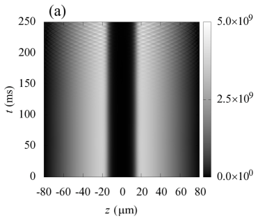
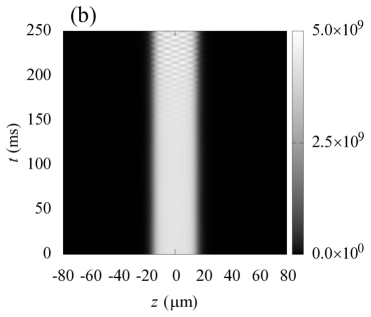
Figure 4: Emergence of Faraday waves in a two-component BEC system in the real-time evolution of longitudinal density profiles: (a) $n_{1}(z,t)$ and (b) $n_{2}(z,t)$. The system is initially in the symbiotic pair state, and is modulated with the amplitude $\epsilon=0.1$ and frequency $\omega=250\times 2\pi$ Hz. The system contains $N_{1}=2.5\cdot 10^{5}$ atoms in the state A and $N_{2}=1.25\cdot 10^{5}$ atoms in the state B, confined by the trap with $\Omega_{\rho 0}=160\times 2\pi$ Hz and $\Omega_{z}=7\times 2\pi$ Hz.

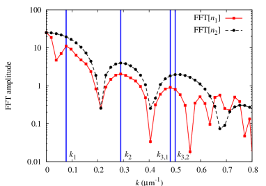
Figure 5: (Color online) Fast Fourier transform of density profiles from Fig. 4 for two condensate components at $t=200$ ms.

In Fig. 4 we show the emergence of Faraday waves in real-time dynamics of a two-component condensate with $N_{1}=2.5\cdot 10^{5}$ atoms in the state A and $N_{2}=1.25\cdot 10^{5}$ atoms in the state B, starting from a symbiotic pair ground state configuration. The magnetic trap has the parameters $\{\Omega_{\rho 0},\Omega_{z}\}=\{160\times 2\pi\,\mbox{ Hz},7\times 2\pi\,\mbox{ Hz}\}$, and we consider the modulation frequency $\omega=250\times 2\pi$ Hz to be far from resonances. The Faraday waves are visible after 150 ms, and we show in Fig. 5 the Fourier spectrum of density profiles of the condensate at $t=200$ ms. The spectrum exhibits several peaks, and the first two peaks, $k_{1}$ and $k_{2}$, common for both components, are related to the geometry of the system. The first peak corresponds to the period $\ell_{1}=2\pi/k_{1}=81.5\,\mu$m, the longitudinal extent of the system, while the second one corresponds to the period $\ell_{2}=2\pi/k_{2}=21.7\,\mu$m, the extent of the central dip in the fist component (or, equivalently, the extent of the second component). The periods of Faraday waves are determined by the peaks $k_{3,j}$, and have very close values, $\ell_{3,1}=13.0\,\mu$m and $\ell_{3,2}=12.5\,\mu$m. The dispersion relation (23) derived in Sec. III.1 indicates a period of $12.0,\mu$m, which is in excellent agreement with the numerical results.

This demonstrates that the variational ansätze from Sec. III.1 were well crafted. The good agreement is also partly due to our normalization of the dark component, where we have used the longitudinal extent of the condensate $L=\ell_{1}$, obtained from the stationary solution of the full set of GPEs. Please note that the emergence of the Faraday waves does not impact the bulk of the condensate, and that its longitudinal extent is constant, which fully justifies our assumption in the variational model.

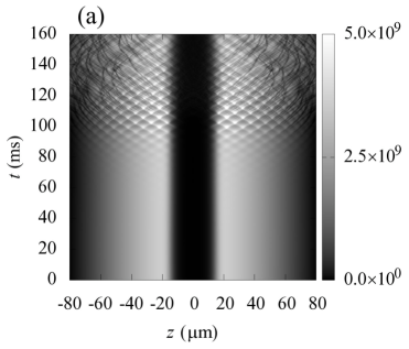
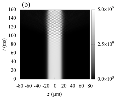
Figure 6: Emergence of resonant waves in a two-component BEC system in the real-time evolution of longitudinal density profiles: (a) $n_{1}(z,t)$ and (b) $n_{2}(z,t)$. The system is initially in the symbiotic pair ground state, and is modulated with the self-resonant frequency $\omega=\Omega_{\rho 0}=160\times 2\pi$ Hz; other parameters as in Fig. 4.

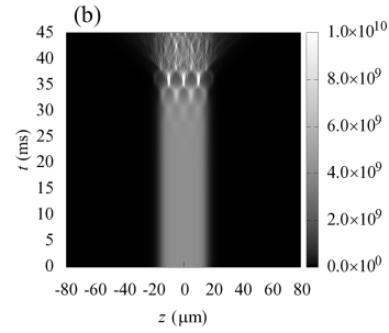
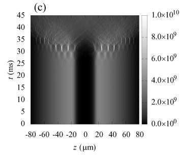
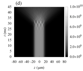
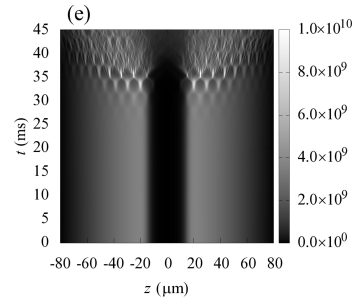
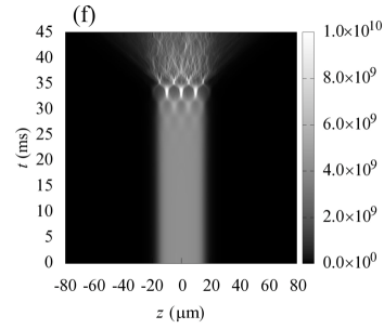
Figure 7: Emergence of resonant waves in a two-component BEC system in the real-time evolution of longitudinal density profiles: $n_{1}(z,t)$ (left column) and $n_{2}(z,t)$ (right column). The system is initially in the symbiotic pair ground state, and is modulated with the frequencies: $\omega=300\times 2\pi$ Hz in (a) and (b); $\omega=2\Omega_{\rho 0}=320\times 2\pi$ Hz in (c) and (d); $\omega=340\times 2\pi$ Hz in (e) and (f). Other parameters are the same as in Fig. 4.

In Fig. 6 we show the resonant dynamics of the condensate for a self-resonance, $\omega=\Omega_{\rho 0}=160\times 2\pi$ Hz. In this case our numerical simulations indicate a narrow resonance where the excited surface waves do not impact the dynamics of the bulk of the condensate. The resonant waves develop faster than the Faraday waves, and already after 70 ms are clearly visible. However, in Fig. 7 we see that for a second resonance at $\omega\approx 2\Omega_{\rho 0}$, the excited surface waves appear even much earlier, after only 25 ms, but are quite short-lived, and the collective dynamics of the two components then takes over. This figure also illustrates that the second resonance is very broad, and covers the interval wider than $40\times 2\pi$ Hz, centered at $2\Omega_{\rho 0}=320\times 2\pi$ Hz.

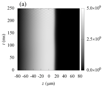
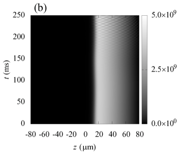
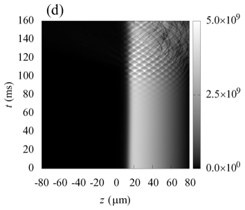
Figure 8: Emergence of Faraday (a, b) and resonant (c, d) waves in a two-component BEC system in the real-time evolution of longitudinal density profiles: $n_{1}(z,t)$ (left column) and $n_{2}(z,t)$ (right column). The system is initially in the segregated excited state, and is modulated with the amplitude $\epsilon=0.1$ and frequencies: $\omega=250\times 2\pi$ Hz in (a) and (b); $\omega=\Omega_{\rho 0}=160\times 2\pi$ Hz in (c) and (d). The system contains $N_{1}=2.5\cdot 10^{5}$ atoms in the state A and $N_{2}=1.25\cdot 10^{5}$ atoms in the state B, and is confined by the trap with $\Omega_{\rho 0}=160\times 2\pi$ Hz and $\Omega_{z}=7\times 2\pi$ Hz.

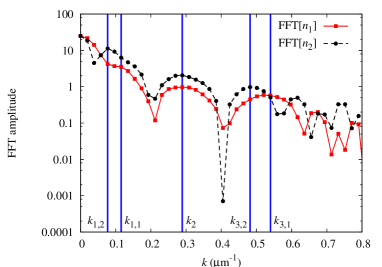
Figure 9: (Color online) Fast Fourier transform of density profiles from Fig. 8 for two condensate components at $t=200$ ms.

We note, in particular, that precisely at the second resonance the two components explode into one another (due to the resonant energy transfer), thereby becoming effectively miscible. This resonant transition to miscibility is specific to two-component systems, and has also been recently reported in binary dipolar BECs TransToMisc . Our analytical treatment of the surface waves indicates a period of $9.3\,\mu$m for the self-resonance, while the full GPEs numerically yield periods of $9.3\,\mu$m for the first component and $9.0\,\mu$m for the second component, which is again an excellent agreement. For the broad resonance at $\omega\approx 2\Omega_{\rho 0}$, the variational treatment gives $4.9\,\mu$m, while numerically we find periods of $9.6\,\mu$m for both components. Here the agreement is only qualitative, due to a violent dynamics observed numerically, which cannot be fully captured by simple ansätze used in Sec. III.1.

As symbiotic states are routinely obtained in ⁸⁷Rb condensates DBSolitonFirstExp ; DarkBrightPhysLettA , the observation of the Faraday waves is definitely within the current experimental capabilities, as is the observation of self-resonant waves at $\omega=\Omega_{\rho 0}$. The observation of resonant waves for $\omega$ close to the second resonance $2\Omega_{\rho 0}$ seems, however, unlikely, as these waves quickly fade out in favor of a forceful resonant dynamics that takes the condensate into the miscible regime and can, for longer timescales, turn the condensate unstable.

IV.2 Segregated states

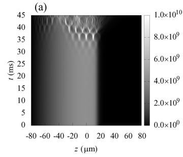
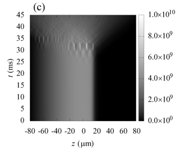
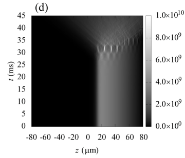
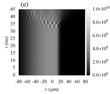
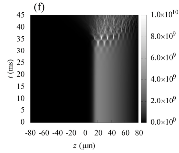
Figure 10: Emergence of resonant waves in a two-component BEC system in the real-time evolution of longitudinal density profiles: $n_{1}(z,t)$ (left column) and $n_{2}(z,t)$ (right column). The system is initially in the segregated excited state, and is modulated with the frequencies: $\omega=300\times 2\pi$ Hz in (a) and (b); $\omega=2\Omega_{\rho 0}=320\times 2\pi$ Hz in (c) and (d); $\omega=340\times 2\pi$ Hz in (e) and (f). Other parameters are the same as in Fig. 8.

In Figs. 8a and 8b and we show the formation of Faraday waves at $\omega=250\times 2\pi$ Hz for a segregated initial state using the same experimental setup as in the previous case. The waves again appear after roughly 150 ms and we show in Fig. 9 the Fourier spectrum of the longitudinal density profile at $t=200$ ms. The spectrum’s two peaks $k_{1,1}$ and $k_{1,2}$ correspond to longitudinal extents of components, $81.5\,\mu$m and $54.3\,\mu$m, while the peak $k_{2}$ corresponds to the width of the interface area between the components of $21.7\,\mu$m.

Periods of the Faraday waves are determined by the peaks $k_{3,1}$ and $k_{3,2}$, and have the values $11.6\,\mu$m for the first and $13.0\,\mu$m for the second component. The dispersion relation derived in Sec. III.2 indicates a period of $16.8\,\mu$m, which overestimates the previous result by roughly 30% due to several reasons: the ansätze we use in Sec. III.2 for two components are symmetric around $z=0$, they have the same normalization, and also they exhibit the Gaussian exponential cut-off away from the center of the trap. From Fig. 3 we already see that these are simplifications made only to ensure analytical tractability of the variational calculation. We also stress that both components are in the Thomas-Fermi regime, hence their wave functions are well-localized and show a distinct quasi-singular cut-off at borders of the cloud, not the Gaussian-type tail. However, even with these simplifications, the variational approach is able to give reasonable estimate for the period of Faraday waves.

We also numerically study resonant dynamics of the two-component BEC system for the self-resonance at $\omega=\Omega_{\rho 0}$. In Figs. 8c and 8d we show real-time evolution of density profiles for both components. The resonance is relatively narrow and the excited surface wave do not impact the overall dynamics of the condensate. The resonant surface waves appear after around 80 ms, and have the period of $11.2\,\mu$m in the first and $12.5\,\mu$m in the second component, while the variational approach, Eq. (37), gives the period of $13.1\,\mu$m. The agreement is quite good, but only coincidental, since we know that the ansätze used in Sec. III.2 are oversimplified, and that we cannot expect more than an order of magnitude agreement.

In the case of a second resonance at $\omega=2\Omega_{\rho 0}$, the excited surface waves fade out in favor of the forceful resonant dynamics that turns the two components miscible. The resonant waves appear already after around 25 ms, much faster than for the self-resonance. As in the case of the symbiotic pair state, the second resonance is much broader than the self-resonance, with the width of more than $40\times 2\pi$ Hz, as illustrated in Fig. 10. Our analytical treatment of the surface waves indicates a period of $6.6\,\mu$m, while the Fourier analysis of the full numerical solution of GPEs yield periods of $10.2\,\mu$m in the first and $9.6\,\mu$m in the second component. As expected, the variational treatment gives a fair estimate of the period of resonant surface waves.

V Conclusions

We have shown the emergence of Faraday waves in binary non-miscible BECs subject to periodic modulations of the transverse confinement. Considering the $\left|1,-1\right\rangle$ and $\left|2,1\right\rangle$ hyperfine states of realistic ⁸⁷Rb condensates, we have shown that there are two types of experimentally relevant stationary configurations: a symbiotic pair ground state, where one component is trapped by the other, and a configuration where the components are well segregated, which represents a first excited state of the system. For both types of configurations we have shown by extensive numerical study that the surface waves in the two components emerge simultaneously, are of similar periods and do not impact the dynamics of the bulk of condensate far from resonances. We have derived analytically periods of the excited surface waves using first a variational treatment of the full system of coupled GPEs that reduced the dynamics of the condensate to a set of coupled ordinary differential equations, and then using a Mathieu-type analysis of these equations we have determined the most unstable solutions. The obtained analytical results for periods of surface waves are shown to give excellent estimates by comparison with the Fourier analysis of numerical solutions of the full set of GPEs. The resonant dynamics seen for modulations equal to the radial trapping frequency (self-resonance), as well as to twice this value (second resonance) were investigated numerically, and we have found that the emergent resonant surface waves appear much faster than the Faraday waves. Using the variational approach developed in Sec. III, the periods of resonant surface waves can be also estimated, and are found to be in reasonable agreement with the numerical results. In the case of a second resonance, the emergent surface waves for both types of initial configurations are found to fade out in favor of a forceful resonant dynamics that turns the binary condensate miscible. This is an interesting phenomenon, and we believe that GPE framework captures its dynamics quite well, similarly to e.g. Ref. collision , where the condensate was split into two separated regions and then the collisional dynamics of the two halves was observed and found to be in excellent agreement with GPE predictions.

Extending the present investigation to experimental setups with anisotropic transverse confinement (such as the one in Ref. DarkBrightPhysLettA ) presents one of interesting venues for future studies. As fully three-dimensional simulations are extremely time-consuming, a natural first step would be to extend the existing (cylindrically symmetric) non-polynomial Schrödinger equations salanischboris ; MateoDelgado to cover the dynamics of binary BECs subject to anisotropic transverse confinement. Also in this direction the study of predominantly two-dimensional (pancake-shaped) condensates has the potential to uncover a rich variety of patterns, and one could even expect the formation of spatio-temporal chaos in such systems. Finally, another natural extension of this work would be to consider parametric resonances and the ensuing Faraday waves in miscible condensates. In this setting the dynamics of the waves in the two components can be mapped variationally onto a set of coupled Mathieu equations whose most unstable solutions are, however, not known analytically.

- (1) M. Faraday, Philos. Trans. R. Soc. London 121, 299 (1831). Related experiments by Chladni and Ørsted are also described in detail in this reference.
- (2) M. C. Cross and P. C. Hohenberg, Rev. Mod. Phys. 65, 851 (1993).
- (3) J. J. García-Ripoll, V. M. Pérez-García, and P. Torres, Phys. Rev. Lett. 83, 1715 (1999).
- (4) K. Staliunas, S. Longhi, and G. J. de Valcárcel, Phys. Rev. Lett. 89, 210406 (2002) .
- (5) K. Staliunas, S. Longhi, and G.J. de Valcárcel, Phys. Rev. A 70, 011601(R) (2004).
- (6) M. Kramer, C. Tozzo, and F. Dalfovo, Phys. Rev. A 71, 061602(R) (2005).
- (7) C. Tozzo, M. Kramer, and F. Dalfovo, Phys. Rev. A 72, 023613 (2005).
- (8) M. Modugno, C. Tozzo, and F. Dalfovo, Phys. Rev. A 74, 061601(R) (2006).
- (9) H. Abe, T. Ueda, M. Morikawa, Y. Saitoh, R. Nomura, and Y. Okuda, Phys. Rev. E 76, 046305 (2007); T. Ueda, H. Abe, Y. Saitoh, R. Nomura, and Y. Okuda, J. Low Temp. Phys. 148, 553 (2007).
- (10) P. Engels, C. Atherton, and M. A. Hoefer, Phys. Rev. Lett. 98, 095301 (2007).
- (11) P. G. Kevrekidis, D. J. Frantzeskakis, and R. Carretero-González (Eds.), Emergent Nonlinear Phenomena in Bose-Einstein Condensates (Springer-Verlag, Berlin, 2008); see also the review R. Carretero-González, D. J. Frantzeskakis, and P. G. Kevrekidis, Nonlinearity 21, R139 (2008).
- (12) X.-J. Liu, H. Hu, A. Minguzzi, and M. P. Tosi, Phys. Rev. A 69, 043605 (2004).
- (13) B. Malomed, Soliton Management in Periodic Systems (Springer, New York, 2006).
- (14) M. D. Petrović, G. Gligorić, A. Maluckov, Lj. Hadžievski, and B. A. Malomed, Phys. Rev. E 84, 026602 (2011).
- (15) A. I. Nicolin, R. Carretero-González, and P. G. Kevrekidis, Phys. Rev. A 76, 063609 (2007).
- (16) A. B. Bhattacherjee, Phys. Scr. 78, 045009 (2008).
- (17) A. I. Nicolin and M. C. Raportaru, Physica A 389, 4663 (2010).
- (18) R. Nath and L. Santos, Phys. Rev. A 81, 033626 (2010).
- (19) P. Capuzzi, M. Gattobigio, and P. Vignolo, Phys. Rev. A 83, 013603 (2011).
- (20) S.-G. Peng, S. S. Bohloul, X.-J. Liu, H. Hu, and P. D. Drummond, Phys. Rev. A 82, 063633 (2010).
- (21) N. Katz and O. Agam, New J. Phys. 12, 073020 (2010).
- (22) E. Diaz, C. Gaul, R. P. A. Lima, F. Dominguez-Adame, and C. A. Müller, Phys. Rev. A 81, 051607(R) (2010).
- (23) G. A. Sekh, e-print arXiv:1109.1117 (2011).
- (24) D.-S. Wang, S.-W. Song, B. Xiong, and W. M. Liu, Phys. Rev. A 84, 053607 (2011).
- (25) C. Gaul, R. P. A. Lima, E. Diaz, C. A. Müller, and F. Dominguez-Adame, Phys. Rev. Lett. 102, 255303 (2009).
- (26) C. Gaul, E. Diaz, R. P. A. Lima, F. Dominguez-Adame, and C. A. Müller, Phys. Rev. A 84, 053627 (2011).
- (27) K. Staliunas, Phys. Rev. A 84, 013626 (2011).
- (28) L. Salasnich, N. Manini, F. Bonelli, M. Korbman, and A. Parola, Phys. Rev A 75, 043616 (2007).
- (29) A. Imambekov, I. E. Mazets, D. S. Petrov, V. Gritsev, S. Manz, S. Hofferberth, T. Schumm, E. Demler, and J. Schmiedmayer, Phys. Rev. A 80, 033604 (2009).
- (30) J. Kronjäger, C. Becker, P. Soltan-Panahi, K. Bongs, and K. Sengstock, Phys. Rev. Lett. 105, 090402 (2010).
- (31) P. Capuzzi and P. Vignolo, Phys. Rev. A 78, 043613 (2008).
- (32) R. A. Tang, H. C. Li, and J. K. Xue, J. Phys. B: At. Mol. Opt. Phys. 44, 115303 (2011).
- (33) C. D. Graf, G. Weick, and E. Mariani, EPL 89, 40005 (2010).
- (34) S. E. Pollack, D. Dries, R. G. Hulet, K. M. F. Magalhaes, E. A. L. Henn, E. R. F. Ramos, M. A. Caracanhas, and V. S. Bagnato, Phys. Rev. A 81, 053627 (2010).
- (35) I. Vidanović, A. Balaž, H. Al-Jibbouri, and A. Pelster, Phys. Rev. A 84, 013618 (2011).
- (36) J. Petrović, I. Herrera, P. Lombardi, and F. S. Cataliotti, e-print arXiv:1111.4321 (2011).
- (37) C. J. Pethick and H. Smith, Bose-Einstein Condensation in Dilute Gases (Cambridge University Press, Cambridge, 2008).
- (38) B. J. Verhaar, E. G. M. van Kempen, and S. J. J. M. F. Kokkelmans, Phys. Rev. A 79, 032711 (2009).
- (39) S. Middelkamp, J. J. Chang, C. Hamner, R. Carretero-González, P. G. Kevrekidis, V. Achilleos, D. J. Frantzeskakis, P. Schmelcher, and P. Engels, Phys. Lett. A 375, 642 (2011).
- (40) C. Hamner, J. J. Chang, P. Engels, and M. A. Hoefer, Phys. Rev. Lett. 106, 065302 (2011).
- (41) A. Bogojević, I. Vidanović, A. Balaž, and A. Belić, Phys. Lett. A 372, 3341 (2008).
- (42) A. Balaž, A. Bogojević, I. Vidanović, and A. Pelster, Phys. Rev. E 79, 036701 (2009).
- (43) I. Vidanović, A. Bogojević, and A. Belić, Phys. Rev. E 80, 066705 (2009).
- (44) I. Vidanović, A. Bogojević, A. Balaž, and A. Belić, Phys. Rev. E 80, 066706 (2009).
- (45) A. Balaž, I. Vidanović, A. Bogojević, and A. Pelster, Phys. Lett. A 374, 1539 (2010).
- (46) P. Muruganandam and S. K. Adhikari, Comp. Phys. Comm. 180, 1888 (2009).
- (47) G. Csire, D. Schumayer, and B. Apagyi, Phys. Rev. A 82, 063608 (2010).
- (48) V. Schweikhard, I. Coddington, P. Engels, S. Tung and E. A. Cornell, Phys. Rev. Lett. 93, 210403 (2004).
- (49) K. J. H. Law, P. G. Kevrekidis, and L. S. Tuckerman, Phys. Rev. Lett. 105, 160405 (2010).
- (50) P. Ao and S. T. Chui, Phys. Rev. A 58, 4836 (1998).
- (51) L. Wang and C. C. Yang, Opt. Lett. 15, 474 (1990).
- (52) Y. S. Kivshar, Opt. Lett. 17, 1322 (1992).
- (53) Z. Chen, M. Segev, T. H. Coskun, D. N. Christodoulides, Y. S. Kivshar, V. V. Afanasjev, Opt. Lett. 21, 1821 (1996).
- (54) Th. Busch and J. R. Anglin, Phys. Rev. Lett. 87, 010401 (2001).
- (55) C. Becker, S. Stellmer, P. Soltan-Panahi, S. Dörscher, M. Baumert, E.-M. Richter, J. Kronjäger, K. Bongs, and K. Sengstock, Nature Phys. 4, 496 (2008).
- (56) H. E. Nistazakis, D. J. Frantzeskakis, P. G. Kevrekidis, B. A. Malomed, and R. Carretero-González, Phys. Rev. A 77, 033612 (2008).
- (57) C. Yin, N. G. Berloff, V. M. Pérez-García, D. Novoa, A. V. Carpentier, and H. Michinel, Phys. Rev. A 83, 051605 (2011).
- (58) D. S. Hall, M. R. Matthews, J. R. Ensher, C. E. Wieman, and E. A. Cornell, Phys. Rev. Lett. 81, 1539 (1998).
- (59) K. M. Mertes, J. W. Merrill, R. Carretero-González, D. J. Frantzeskakis, P. G. Kevrekidis, and D. S. Hall, Phys. Rev. Lett. 99, 190402 (2007).
- (60) D. M. Weld, P. Medley, H. Miyake, D. Hucul, D. E. Pritchard, and W. Ketterle, Phys. Rev. Lett. 103, 245301 (2009).
- (61) A. I. Nicolin and M. C. Raportaru, Proc. Rom. Acad. Ser. A 12, 209 (2011).
- (62) A. I. Nicolin, Rom. Rep. Phys. 63, 1329 (2011).
- (63) A. I. Nicolin, Physica A 391, 1062 (2012).
- (64) V. M. Pérez-García, H. Michinel, J. I. Cirac, M. Lewenstein, and P. Zoller, Phys. Rev. A 56, 1424 (1997).
- (65) N. W. McLachlan, Theory and Application of Mathieu Functions (Oxford University Press, New York, 1951).
- (66) D. Borzov, M. S. Mashayekhi, S. Zhang, J.-L. Song, F. Zhou, e-print arXiv:1110.2183 (2011).
- (67) G. Gligorić, A. Maluckov, M. Stepić, Lj. Hadžievski, and B. A. Malomed, Phys. Rev. A 82, 033624 (2010).
- (68) J. J. Chang, P. Engels, and M. A. Hoefer, Phys. Rev. Lett. 101, 170404 (2008).
- (69) L. Salasnich and B. A. Malomed, Phys. Rev. A 74, 053610 (2006).
- (70) A. Muñoz Mateo and V. Delgado, Phys. Rev. A 77, 013617 (2008).