Retrieving the three-dimensional matter power spectrum and galaxy biasing parameters from lensing tomography

Abstract

Aims. With the availability of galaxy distance indicators in weak lensing surveys, lensing tomography can be harnessed to constrain the three-dimensional (3D) matter power spectrum over a range of redshift and physical scale. By combining galaxy-galaxy lensing and galaxy clustering, this can be extended to probe the 3D galaxy-matter and galaxy-galaxy power spectrum or, alternatively, galaxy biasing parameters.

Methods. To achieve this aim, this paper introduces and discusses minimum variance estimators and a more general Bayesian approach to statistically invert a set of noisy tomography two-point correlation functions, measured within a confined opening angle. Both methods are constructed such that they probe deviations of the power spectrum from a fiducial power spectrum, thereby enabling both a direct comparison of theory and data, and in principle the identification of the physical scale and redshift of deviations. By devising a new Monte Carlo technique, we quantify the measurement noise in the correlators for a fiducial survey, and test the performance of the inversion techniques.

Results. For a relatively deep $200\,\rm deg^{2}$ survey ($\bar{z}\sim 0.9$) with 30 sources per square arcmin, the matter power spectrum can be probed with $3-6\sigma$ significance on comoving scales $1\lesssim k\,h^{-1}{\rm Mpc}\lesssim 10$ and $z\lesssim 0.3$. For 3 lenses per square arcmin, a significant detection ($\sim 10\sigma$) of the galaxy-matter power spectrum and galaxy power spectrum is attainable to relatively high redshifts ($z\lesssim 0.8$) and over a wider $k$-range. Within the Bayesian framework, all three power spectra are easily combined to provide constraints on 3D galaxy biasing parameters. Therein, weak priors on the galaxy bias improve constraints on the matter power spectrum.

Conclusions. A shear tomography analysis of weak-lensing surveys in the near future promises fruitful insights into both the effect of baryons on the nonlinear matter power spectrum at $z\lesssim 0.3$ and galaxy biasing ($z\lesssim 0.5$). However, a proper treatment of the anticipated systematics, which are not included in the mock analysis but discussed here, is likely to reduce the signal-to-noise ratio in the analysis such that a robust assessment of the 3D matter power spectrum probably requires a survey area of at least $\sim 10^{3}\,\rm deg^{2}$. To investigate the matter power spectrum at redshift higher than $\sim 0.3$, an increase in survey area is mandatory.

1 Introduction

In the framework of the standard model of cosmology (e.g., Dodelson, 2003), structure in the matter density field evolves over time under the influence of gravitational collapse from a relatively homogeneous state, as for instance observed in the small temperature fluctuations of the cosmic microwave background (CMB; Komatsu et al., 2011), to the highly structured matter density field of today. The main driver of the structure formation is the postulated dark matter, which is the dominant matter component. According to the model, dark matter only interacts by means of either the weak nuclear force or gravity. Moreover, the first galaxies were formed from the subdominant primordial baryonic gas component, building stars within the gravitational potential wells of the dark matter (e.g., Mo et al., 2010), and evolved later on.

To quantify the state of the structure formation process at a given cosmic time or a radial comoving distance $\chi$, the amplitude of the fluctuations

$$\delta_{\rm m}(\@vec{x},\chi)=\frac{\rho_{\rm m}(\@vec{x},\chi)-\bar{\rho}_{\rm m}(\chi)}{\bar{\rho}_{\rm m}(\chi)}$$ (1)

in the matter density field $\rho_{\rm m}(\@vec{x},\chi)$ relative to the mean matter density $\bar{\rho}_{\rm m}(\chi)$, at a comoving position $\@vec{x}$, is expressed by the matter power spectrum $P_{\rm m}(k,\chi)$ (e.g., Martínez & Saar, 2002)

$$\Big{\langle}\tilde{\delta}_{\rm m}(\@vec{k},\chi)\tilde{\delta}_{\rm m}(\@vec{k}^{\prime},\chi)\Big{\rangle}=(2\pi)^{3}\delta_{\rm D}^{(3)}(\@vec{k}+\@vec{k}^{\prime})P_{\rm m}(k,\chi)\;,$$ (2)

where

$$\tilde{\delta}_{\rm m}(\@vec{k},\chi)=\int{\rm d}^{3}x\,\delta_{\rm m}(\@vec{x},\chi){\rm e}^{-{\rm i}\@vec{x}\cdot\@vec{k}}$$ (3)

are the amplitudes of the density modes with wave-number $|\@vec{k}|$ or wave length $2\pi/|\@vec{k}|$, $\delta^{(3)}_{\rm D}(\@vec{x})$ is the Dirac delta function, and $\langle\ldots\rangle$ denotes the ensemble average over all realisations of the matter density field. In the cosmological context, density fields are statistically homogeneous and isotropic.

The matter power spectrum contains a wealth of information directly related to the physics of the matter components in the Universe as well as the primordial density fluctuations (Peacock, 1999, and references therein) and information about possible modifications to Einstein’s general relativity that may affect the growth of the density fluctuations (Uzan & Bernardeau, 2001; Clifton et al., 2011). While the matter power spectrum at redshift $z\sim 1000$ is relatively well-understood theoretically and known empirically from CMB studies (Komatsu et al., 2011), the power spectrum in the more recent Universe on quasi- to nonlinear scales $k\gtrsim 1\,h\rm Mpc^{-1}$ is less well-known: On the theoretical side, the magnitude of the influence of galaxies and baryons seems to be unclear but probably significant (Zhan & Knox, 2004; Jing et al., 2006; Somogyi & Smith, 2010; Semboloni et al., 2011; van Daalen et al., 2011), although predictions for dark-matter-only scenarios are accurate (Peacock & Dodds, 1996; Smith et al., 2003; Heitmann et al., 2010). On the empirical side, detailed studies of the power spectrum in this regime rely mostly on tracers (Tegmark et al., 2004), such as galaxies or absorbers in the Lyman-$\alpha$ forest, which have an uncertain relation to the underlying matter density field. This provides a strong motivation to directly measure either the spatial matter power spectrum or the spatial matter correlation function.

One purpose of this paper is to propose estimators of the matter power spectrum based on the weak gravitational lensing effect to allow a direct measurement of $P_{\rm m}(k,\chi)$, especially in the nonlinear regime. Weak gravitational lensing (Schneider, 2006, for a review) is a tool to study the large-scale distribution of matter by its effect on the shape of distant galaxy images (“sources”). Images of galaxies are weakly distorted (sheared) by the bending of light passing by intervening matter density fluctuations (“lenses”). As the effect is only sensitive to the fluctuations in the gravitational field of intervening matter, it can be employed to probe the matter density field without further knowledge of its physical properties and without the usage of tracers. This makes it an excellent probe to explore the elusive dark matter component or the general composition of matter on cosmological scales (see for example Clowe et al. 2006 or Tereno et al. 2009).

As weak lensing is sensitive to all intervening matter, it naturally measures the projected matter density fluctuations within radial cylinders. Known lensing-based estimators of the matter power spectrum are therefore essentially two-dimensional by either estimating the projected matter fluctuations on the sky (Blandford et al., 1991; Miralda-Escude, 1991; Kaiser, 1992; Schneider et al., 1998; Hu & White, 2001; Schneider et al., 2002; Pen et al., 2002) or translating this into a spatial power spectrum at one effective distance (Pen et al., 2003). With the availability of distance indicators for the sources, one has started to exploit the change in the weak lensing shear $\gamma(\chi_{\rm s})$ as a function of comoving source distance $\chi_{\rm s}$. For a fixed lens distance $\chi_{\rm d}$, this is expressed by

$$\gamma(\chi_{\rm s})\propto\frac{f_{\rm k}(\chi_{\rm s}-\chi_{\rm d})}{f_{\rm k}(\chi_{\rm s})}$$ (4)

with $f_{\rm k}(\chi)$ being the comoving angular diameter distance. The weight of a lens in the total shear signal, including lenses at all distances, therefore varies with a varying source distance. In a cosmic shear tomography analysis, this is utilised to provide improved constraints on cosmological parameters (Hu, 2002; Massey et al., 2007b; Schrabback et al., 2010; Kitching et al., 2011) or to map the three-dimensional (3D) matter density field (Hu & Keeton, 2002; Massey et al., 2007a; VanderPlas et al., 2011; Simon et al., 2012; Leonard et al., 2012) by analysing the lensing signal for a series of source distance slices.

Weak lensing also offers the opportunity to investigate the distribution of cosmological objects in relation to the matter density field. As in the case of the matter power spectrum, one defines the clustering power spectrum of galaxies

$$\Big{\langle}\tilde{\delta}_{\rm g}(\@vec{k},\chi)\tilde{\delta}_{\rm g}(\@vec{k}^{\prime},\chi)\Big{\rangle}=(2\pi)^{3}\delta_{\rm D}^{(3)}(\@vec{k}+\@vec{k}^{\prime})\left(P_{\rm g}(k,\chi)+\frac{1}{\bar{n}_{\rm g}}\right)$$ (5)

and the cross-correlation power of the matter and galaxy distribution

$$\Big{\langle}\tilde{\delta}_{\rm g}(\@vec{k},\chi)\tilde{\delta}_{\rm m}(\@vec{k}^{\prime},\chi)\Big{\rangle}=(2\pi)^{3}\delta_{\rm D}^{(3)}(\@vec{k}+\@vec{k}^{\prime})P_{\delta\rm g}(k,\chi)\;,$$ (6)

based on the galaxy number density contrast $\delta_{\rm g}=n_{\rm g}/\bar{n}_{\rm g}-1$, where $n_{\rm g}$ is the number density of galaxies, and $\bar{n}_{\rm g}$ their mean number density. We note that the definition of $P_{\rm g}(k,\chi)$ separates the Poisson shot noise contribution, originating from the discreteness of the galaxies, from the number density fluctuations (e.g., Peacock, 1999). For galaxies faithfully tracing the distribution of matter, all three power spectra $P_{\delta}(k,\chi)$, $P_{\delta\rm g}(k,\chi)$, and $P_{\rm g}(k,\chi)$ are identical. More generally, however, we have to assume that galaxies are imperfect tracers, i.e., biased tracers, of the matter distribution. Galaxy biasing is commonly expressed at the power spectrum level by the biasing functions $b(k,\chi)$ and $r(k,\chi)$ (e.g., Tegmark & Peebles, 1998):

$$P_{\delta\rm g}(k,\chi) = b(k,\chi)r(k,\chi)P_{\delta}(k,\chi)\;,$$ (7)

$$P_{\rm g}(k,\chi) = b^{2}(k,\chi)P_{\delta}(k,\chi)\;.$$ (8)

Measuring galaxy biasing addresses the question of galaxy formation and evolution as deviations of galaxy clustering from (dark) matter clustering – as reflected by the biasing functions with $b,r\neq 1$ – constrain galaxy models (Yoshikawa et al., 2001; Weinberg et al., 2004; Springel et al., 2005).

Non-parametric weak gravitational-lensing methods have been proposed (van Waerbeke, 1998; Schneider, 1998; Pen et al., 2003) and applied (Hoekstra et al., 2002; Pen et al., 2003; Simon et al., 2007) to assess the galaxy biasing for an effective radial distance, but to date without exploiting tomography. The formalism in this paper is kept general enough to constrain the galaxy biasing functions $b(k,\chi)$ and $r(k,\chi)$ or, alternatively, the power spectra $P_{\delta\rm g}(k,\chi)$ and $P_{\rm g}(k,\chi)$ as well.

To enable the employment of this new tomography technique, the appropriate lensing data will soon be available. Recent, ongoing, and prospective lensing surveys – such as the Canada-France-Hawaii Legacy Survey (CFHTLS), the Panoramic Survey Telescope and Rapid Response System surveys (Pan-STARRS), the Dark Energy Survey (DES), and the Kilo-Degree Survey (KiDS) – will provide between hundreds and thousands of square degrees of shear data endowed with galaxy redshifts. With data sets of this magnitude in hand, we can expect to extract the 3D matter power spectrum and biasing parameters of a selected galaxy population, as discussed in the following.

The paper is structured as follows. Sect. 2 derives a set of minimum variance estimators, which, when applied to measurements of angular correlation functions detailed below, yield constraints on the 3D power spectra $P_{\delta}(k,\chi)$, $P_{\delta\rm g}(k,\chi)$, and $P_{\rm g}(k,\chi)$. In Sect. 2.6, the estimators are applied to a fiducial survey (Sect. 2.4) to forecast their performance. The estimators are improved within a Bayesian analysis in Sect. 3. Sect. 3.2 applies the Bayesian methodology to the fiducial survey. Finally, in Sect. 4 we discuss the results and draw general conclusions.

As a fiducial cosmology, this paper uses a $\Lambda$CDM model (adiabatic fluctuations) with matter density parameter $\Omega_{\rm m}=0.27$, of which baryons are given by $\Omega_{\rm b}=0.046$, a cosmological constant $\Omega_{\Lambda}=1-\Omega_{\rm m}$, and a Hubble parameter $H_{0}=h\,100\,{\rm km}\,{\rm s}^{-1}\,{\rm Mpc}^{-1}$. Length scales are quoted for $h=1$, while the shape parameter of the dark matter clustering adopts $h=0.704$. The normalisation of the matter fluctuations within a sphere of radius $8\,h^{-1}\rm Mpc$ at redshift zero is assumed to be $\sigma_{8}=0.81$. For the spectral index of the primordial matter power spectrum, we use $n_{\rm s}=0.96$.

2 Minimum variance estimators of band power spectra

For extensive recent reviews of weak gravitational lensing and the weak lensing formalism, we refer the reader to Van Waerbeke & Mellier (2003) or Schneider (2006).

As we show in the following, fixing the angular diameter distance $f_{\rm k}(\chi)$, the matter density parameter $\Omega_{\rm m}$, and the relation between comoving radial distance and redshift

$$\chi(z)=\int_{0}^{z}\frac{c{\rm d}z^{\prime}}{H(z^{\prime})}$$ (9)

within a reference fiducial cosmology (where $H(z)$ is the Hubble parameter at redshift $z$), allows us to find a simple linear relation between the 3D power spectra and the angular correlation functions as long as lens-lens couplings are negligible. This is assumed for the scope of this paper.

The lens and source catalogues from a galaxy lensing survey split into $N_{\rm source}$ and $N_{\rm lens}$ subsamples, each covering different radial distance regimes. Quantities computed from the $i$th subsample are referred to in the following by a superindex as in “$q^{(i)}$”. Likewise, quantities computed from a pair of subsamples $i$ and $j$ are denoted by “$q^{(ij)}$”. By tomography, we mean a set of angular two-point correlation functions obtained from pairs of galaxy subsamples. The pair combinations include galaxies from both different and the same redshift bins.

2.1 Matter power spectrum

Here we start with shear-shear correlations between sources (e.g., Schneider, 2006, and references therein)

$$\xi_{\pm}^{(ij)}(|\@vec{\Delta\theta}|)=\Big{\langle}\gamma^{(i)}_{\rm t}(\@vec{\theta})\gamma^{(j)}_{\rm t}(\@vec{\theta}^{\prime})\Big{\rangle}\pm\Big{\langle}\gamma^{(i)}_{\times}(\@vec{\theta})\gamma^{(j)}_{\times}(\@vec{\theta}^{\prime})\Big{\rangle}\;,$$ (10)

where $\gamma^{(i)}_{\times}$ and $\gamma^{(i)}_{\rm t}$ denote the cross and tangential shear component of sources in the $i$th subsample, which are both evaluated relative to the line $\@vec{\Delta\theta}=\@vec{\theta}^{\prime}-\@vec{\theta}$ connecting the two sources in directions $\@vec{\theta}$ and $\@vec{\theta}^{\prime}$. For shear fields and positions on the (flat) sky, we employ the complex notation, which is widely used in the literature. The source catalogue is split into $N_{\rm source}$ subsamples with known radial distributions $p_{\chi}^{(i)}(\chi)$ that define the probability of finding a source within the comoving distance interval $[\chi,\chi+{\rm d}\chi]$ by $p_{\chi}^{(i)}(\chi){\rm d}\chi$.

Using Limber’s approximation (Kaiser, 1992), the $\xi_{\pm}^{(ij)}(\theta)$ in the shear tomography can be related to the 3D matter power spectrum as in (e.g., Simon et al., 2004)

$$\xi_{\pm}^{(ij)}(\theta)=$$

$$\frac{9H_{0}^{4}\Omega_{\rm m}^{2}}{4c^{4}}\int_{0}^{\chi_{\rm h}}\!\!\!\!\int_{0}^{\infty}\frac{{\rm d}\chi{\rm d}\ell\,\ell}{2\pi}\frac{\overline{W}^{(i)}(\chi)\overline{W}^{(j)}(\chi)}{a(\chi)}J_{0,4}(\ell\theta)P_{\delta}\left(\frac{\ell}{f_{\rm k}(\chi)},\chi\right)\;,$$

where the average lensing efficiency is defined as

$$\overline{W}^{(i)}(\chi)=\int_{\chi}^{\chi_{\rm h}}{\rm d}\chi^{\prime}p_{\chi}^{(i)}(\chi^{\prime})\frac{f_{\rm k}(\chi^{\prime}-\chi)}{f_{\rm k}(\chi^{\prime})}\;.$$ (12)

We have also introduced $a(\chi)$ as the cosmic scale factor at comoving distance $\chi$, the $n$th-order Bessel function of the first kind $J_{n}(x)$, and the comoving radius of the observable Universe $\chi_{\rm h}$.

Moving on to expand the 3D matter power spectrum $P_{\delta}(k,\chi)$ as a linear combination of basis functions, we define a 2D grid with grid points $(k_{m},\chi_{n})$ and $m\in\{1,\ldots,N_{k}+1\},n\in\{1,\ldots,N_{z}+1\}$. The grid positions are sorted, $k_{m}<k_{m+1}$ and $\chi_{n}<\chi_{n+1}$. The grid points mark the interval limits of a band power spectrum. To focus on deviations from a model power spectrum, the band powers are defined relative to a fiducial matter power spectrum $P^{\rm fid}_{\delta}(k,\chi)$ that describes the expected variation in the power within the bands or regions outside the grid

$$P_{\delta}(k,\chi) = P^{\rm fid}_{\delta}(k,\chi)\left(1+\sum_{n=1}^{N_{z}}\sum_{m=1}^{N_{k}}H_{mn}(k,\chi)\left[f_{\delta,mn}-1\right]\right)\;,$$ (13)

where $f_{\delta,mn}$ are factors allowing a deviation from the fiducial band powers, and

$$H_{mn}(k,\chi):=\left\{\begin{array}[]{ll}1&{\rm if}\leavevmode\nobreak\ k\in[k_{m},k_{m+1}[\leavevmode\nobreak\ {\rm and}\leavevmode\nobreak\ \chi\in[\chi_{n},\chi_{n+1}[\\ 0&{\rm otherwise}\end{array}\right.$$ (14)

defines a 2D top hat function. Therefore, $P_{\delta}(k,\chi)$ is approximated by in total $N_{k}N_{z}$ free parameters $f_{\delta,\rm mn}$. The boundaries $(k_{1},k_{N_{k}+1})$ and $(\chi_{1},\chi_{N_{z}+1})$ confine the range that is allowed to be modified in comparison to the fiducial model. According to Eq. (13), outside this region one has only $P_{\delta}(k,\chi)=P^{\rm fid}_{\delta}(k,\chi)$. Inside the region, a value of $f_{\delta,mn}=1$ uses either the power expected from the fiducial model or a different power amplitude. In this paper, we focus in particular on evaluating the coefficients $f_{\delta,mn}$ and similar coefficients for other power spectra we introduce below. We note that by setting $P^{\rm fid}_{\delta}(k,\chi)\equiv 1$ and the grid being sufficiently large, we approximate the matter power spectrum by constant powers within the band with absolute amplitudes $f_{\delta,mn}$. Adopting a concrete fiducial model spectrum as a reference may, however, be more advantageous as it implements trends in $k$ and $\chi$ within the (broad) bands as expected from theory. If the trends (not the absolute amplitudes) are more or less realistic, we can expect the factors $f_{\delta,mn}$ to be only slowly changing functions of either $k$ or $\chi$. Moreover, the fiducial model makes the reconstruction more stable as it specifies the power spectrum within a $k$-regime that is only poorly constrained owing to the limited angular range that is covered by the angular correlation function. For the scope of this paper, where $f_{\delta,\rm mn}=1$ is constant throughout, we keep the number of bins with $N_{z}=5$ (linear) and $N_{k}=10$ (log-bins) relatively small.

By virtue of this band power approximation, Eq. (2.1) can be cast into the linear form

$$\xi_{\pm}^{(ij)}(\theta)=\sum_{n=1}^{N_{z}}\sum_{m=1}^{N_{k}}X^{(ij)}_{\pm}(\theta;m,n)f_{\delta,mn}+\xi_{\pm,\rm fid}^{(ij)}(\theta)\;,$$ (15)

where we utilise the basis functions

$$X^{(ij)}_{\pm}(\theta;m,n):=\frac{9H_{0}^{4}\Omega_{\rm m}^{2}}{8\pi c^{4}\theta^{2}}\,\times$$

$$\int_{\chi_{n}}^{\chi_{n+1}}{\rm d}\chi\frac{\overline{W}^{(i)}(\chi)\overline{W}^{(j)}(\chi)}{a(\chi)}\int\limits_{k_{m}f_{\rm k}(\chi)\theta}^{k_{m+1}f_{\rm k}(\chi)\theta}{\rm d}s\,s\,J_{0,4}(s)\,P^{\rm fid}_{\delta}\left(\frac{s}{f_{\rm k}(\chi)\theta},\chi\right)\;;$$

the Bessel function $J_{0}$ is used for $X^{(ij)}_{+}$, whereas $J_{4}$ has to be used in the case of $X^{(ij)}_{-}$. A short description of the numerical evaluation of this integral and similar integrals to follow can be found in Appendix A. The fiducial correlation function $\xi_{\pm,\rm fid}^{(ij)}$ accounts for any possible invariable contributions from the $(k,\chi)$-plane that are not covered by the grid

$$\xi_{\pm,\rm fid}^{(ij)}(\theta):=\frac{9H_{0}^{4}\Omega_{\rm m}^{2}}{8\pi c^{4}\theta^{2}}\,\times$$

$$\int_{0}^{\chi_{\rm h}}{\rm d}\chi\frac{\overline{W}^{(i)}(\chi)\overline{W}^{(j)}(\chi)}{a(\chi)}\int\limits_{0}^{\infty}{\rm d}s\,s\,J_{0,4}(s)\,\cancel{P}^{\rm fid}_{\delta}\left(\frac{s}{f_{\rm k}(\chi)\theta},\chi\right)\;,$$

where

$$\cancel{P}^{\rm fid}_{\delta}\left(k,\chi\right):=\left\{\begin{array}[]{ll}P^{\rm fid}_{\delta}(k,\chi)&,\leavevmode\nobreak\ {\rm if}\leavevmode\nobreak\ \sum\limits_{m,n=1}^{N_{z},N_{k}}H_{mn}(k,\chi)=0\\ 0&,\leavevmode\nobreak\ {\rm otherwise}\end{array}\right.\;.$$ (18)

For sufficiently large grids as in the mock analysis below, however, we find this contribution to be negligible.

In practise, one obtains a measurement of $\xi_{\pm}^{(ij)}(\theta_{l})$ for a series of $l\in\{1,\ldots,N_{\theta}\}$ $\theta$-bins and $N_{\rm source}(N_{\rm source}+1)/2$ combinations of source subsamples $(ij)$. After arranging the series of data points as one compact shear tomography data vector $\@vec{\xi}$ with $N_{\theta}N_{\rm source}(N_{\rm source}+1)$ elements, the set of equations in Eq. (15) for all index pairs $(ij)$ can be written as

$$\@vec{\xi}={\@tens{X}}\@vec{f}_{\delta}+\@vec{\xi}_{\rm fid}\;.$$ (19)

Here, the band power factors $f_{\delta.mn}$, compiled within the vector $\@vec{f}_{\delta}$, and the matrix elements of ${\@tens{X}}$, consisting of the $X_{\pm}^{(ij)}(\theta_{l};m,n)$, are arranged to comply with the structure of $\@vec{\xi}$. The constant vector $\@vec{\xi}_{\rm fid}$ consists of the fiducial correlation-function values $\xi^{(ij)}_{\pm,\rm fid}(\theta_{l})$.

For a given noisy $\@vec{\xi}$ from observation, this equation has to be inverted with respect to $\@vec{f}_{\delta}$. As an estimator for $\@vec{f}_{\delta}$, we suggest a minimum variance estimator (cf. Zaroubi et al., 1995)

$$\hat{\@vec{f}}_{\delta}=[{\@tens{X}}^{\rm t}{\@tens{N}}_{\xi}^{-1}{\@tens{X}}]^{-1}{\@tens{X}}^{\rm t}{\@tens{N}}^{-1}_{\xi}\left(\@vec{\xi}-\@vec{\xi}_{\rm fid}\right)\;,$$ (20)

which minimises the residual $\langle||\hat{\@vec{f}}_{\delta}-\@vec{f}_{\delta})||^{2}\rangle$, the average over all noise realisations, where $||\ldots||$ is the Euclidean norm. Compared to the simple inverse ${\@tens{X}}^{-1}$, the estimator can also cope if the system of linear equations in Eq. (19) is over-determined. In this case, redundant information is optimally combined based on the noise covariance

$${\@tens{N}}_{\xi}:=\Big{\langle}\left(\@vec{\xi}-\langle\@vec{\xi}\rangle\right)\left(\@vec{\xi}-\langle\@vec{\xi}\rangle\right)^{\rm t}\Big{\rangle}\;.$$ (21)

The covariance of the estimator is

$${\@tens{N}}_{\delta}=\Big{\langle}\@vec{\hat{f}}_{\delta}\@vec{\hat{f}}^{\rm t}_{\delta}\Big{\rangle}-\Big{\langle}\@vec{\hat{f}}_{\delta}\Big{\rangle}\Big{\langle}\@vec{\hat{f}}^{\rm t}_{\delta}\Big{\rangle}=[{\@tens{X}}^{\rm t}{\@tens{N}}_{\xi}^{-1}{\@tens{X}}]^{-1}\;,$$ (22)

which can be used to quantify the error and the correlation of errors in the estimate. Furthermore, the estimator is unbiased when $\@vec{\xi}_{\rm fid}$ is correct.

The estimator will fail when the matrix product in the square brackets of ${\@tens{N}}_{\delta}$ is singular, which happens when the problem is ill-conditioned. In this context, ill-conditioned can mean that either $\@vec{f}_{\delta}$ comprises a redshift or length-scale range that is unconstrained by $\@vec{\xi}$, or the impact of different bands on $\@vec{\xi}$ is entirely degenerate. One usually has to modify the $(k_{m},\chi_{n})$ band boundaries, the redshift slicing, or the fiducial power spectrum $P^{\rm fid}_{\delta}(k,\chi)$ accordingly to remove the singularity. To evade the problem of the undefined estimator, we use a singular-value decomposition (SVD; Press et al., 1992) for the inversion of ${\@tens{X}}^{\rm t}{\@tens{N}}_{\xi}^{-1}{\@tens{X}}$ in order to find a pseudo-inverse. The pseudo-inverse ${\@tens{A}}^{+}$ of a matrix ${\@tens{A}}$ minimises the matrix norm $||{\@tens{A}}{\@tens{A}}^{+}-{\@tens{1}}||$, where ${\@tens{1}}$ is the unity matrix. For a regular matrix ${\@tens{A}}$, the straightforward solution is ${\@tens{A}}^{+}={\@tens{A}}^{-1}$. For a singular ${\@tens{A}}$, on the other hand, a solution $\@vec{x}^{+}={\@tens{A}}^{+}\@vec{b}$ is constrained to be as close as possible to ${\@tens{A}}\@vec{x}=\@vec{b}$.

For the problem at hand, the pseudo-inverse can yield a biased estimator for the unconstrained or degenerate parts of $\@vec{f}_{\delta}$. To determine the biased elements in $\hat{\@vec{f}}_{\delta}$, we use as reference

$$\@vec{f}^{\rm ref}_{\delta}=[{\@tens{N}}_{\delta}^{-1}]^{+}{\@tens{N}}_{\delta}^{-1}\@vec{1}\;,$$ (23)

where $\@vec{1}$ is a vector with the same number of elements as $\@vec{f}_{\delta}$ but with all elements set to unity; this is the estimator in Eq. (20) applied to the data vector $\@vec{\xi}_{\rm test}={\@tens{X}}\@vec{1}+\@vec{\xi}_{\rm fid}$ that is expected from the fiducial reference model. The elements in $\@vec{f}^{\rm ref}_{\delta}$ that are unity are either unbiased or biased.

2.2 Galaxy-matter cross-correlation power spectrum

A line of reasoning similar to that in Sect. 2.1 also applies to the galaxy-matter cross-correlation power spectrum $P_{\delta\rm g}(k,\chi)$. A projection of the 3D matter-galaxy power spectrum $P_{\delta\rm g}$ is measured by estimating the mean tangential shear $\overline{\gamma}_{\rm t}$ about a sample of lenses with a number density contrast

$$\kappa_{\rm g}(\@vec{\theta})=\frac{n_{\rm g}(\@vec{\theta})}{\overline{N}_{\rm g}}-1$$ (24)

on the sky, namely (Bartelmann & Schneider, 2001)

$$\bar{\gamma}_{\rm t}(|\@vec{\Delta\theta}|)+{\rm i}\bar{\gamma}_{\times}(|\@vec{\Delta\theta}|)=-{\rm e}^{-2{\rm i}\phi}\Big{\langle}\kappa_{\rm g}(\@vec{\theta}^{\prime})\gamma(\@vec{\theta})\Big{\rangle}\;,$$ (25)

where $\overline{\gamma}_{\rm t}(\Delta\theta)$ (mean tangential shear) denotes the mean shear around a lens at separation $\Delta\theta$ in a reference frame rotated by the angle defined by the polar angle $\phi$ of $\@vec{\Delta\theta}:=\@vec{\theta}-\@vec{\theta}^{\prime}$, $\bar{\gamma}_{\times}$ is the mean cross-shear component (mean cross shear), which cannot be generated to lowest order by gravitational lensing and may be used as reliable indicator of systematics, and $n_{\rm g}(\@vec{\theta})$ denotes the lens number density on the sky in the direction of $\@vec{\theta}$ and $\overline{N}_{\rm g}=\langle n_{\rm g}(\@vec{\theta})\rangle$ the mean lens number density. The mean tangential or cross shear do not rely on $\phi$ owing to the statistical isotropy of the fields.

For galaxy samples sliced in redshift with sources from the $i$th sample and lenses from the $j$th sample, the relation of $\bar{\gamma}^{(ij)}_{\rm t}(\theta)$ to the 3D matter-galaxy cross-power spectrum is (e.g., Simon et al., 2007)

$$\overline{\gamma}_{\rm t}^{(ij)}(\theta)=$$

$$\frac{3H_{0}^{2}\Omega_{\rm m}}{2c^{2}}\int_{0}^{\chi_{\rm h}}\!\!\!\!\int_{0}^{\infty}\frac{{\rm d}\chi{\rm d}\ell\,\ell}{2\pi}\frac{\overline{W}^{(i)}(\chi)q_{\chi}^{(j)}(\chi)}{f_{\rm k}(\chi)a(\chi)}J_{2}(\ell\theta)P_{\delta\rm g}\left(\frac{\ell}{f_{\rm k}(\chi)},\chi\right)\;.$$

As before with the sources, we need to know the radial (probability) distribution $q^{(j)}_{\chi}(\chi)$ for each lens slice.

If we fix the fiducial cosmological model and adopt for $P_{\delta\rm g}(k,\chi)$ the previous band power Ansatz in Eq. (13) with free scaling parameters $f_{{\delta\rm g},mn}$ relative to a fiducial power spectrum, we now obtain

$$\overline{\gamma}_{\rm t}^{(ij)}(\theta)=\sum_{n=1}^{N_{z}}\sum_{m=1}^{N_{k}}Y^{(ij)}(\theta;m,n)f_{{\delta\rm g},mn}+\overline{\gamma}_{\rm t,fid}^{(ij)}(\theta)$$ (27)

with the basis functions

$$Y^{(ij)}(\theta;m,n)=\frac{3H_{0}^{2}\Omega_{\rm m}}{4\pi c^{2}\theta^{2}}\,\times$$

$$\int_{\chi_{n}}^{\chi_{n+1}}{\rm d}\chi\frac{\overline{W}^{(i)}(\chi)q_{\chi}^{(j)}(\chi)}{f_{\rm k}(\chi)a(\chi)}\int\limits_{k_{m}f_{\rm k}(\chi)\theta}^{k_{m+1}f_{\rm k}(\chi)\theta}{\rm d}s\,s\,J_{2}(s)\,P^{\rm fid}_{\delta}\left(\frac{s}{f_{\rm k}(\chi)\theta},\chi\right)\;,$$

and the invariable terms

$$\overline{\gamma}_{\rm t,fid}^{(ij)}(\theta):=\frac{3H_{0}^{2}\Omega_{\rm m}}{4\pi c^{2}\theta^{2}}\,\times$$

$$\int_{0}^{\chi_{\rm h}}{\rm d}\chi\frac{\overline{W}^{(i)}(\chi)q_{\chi}^{(j)}(\chi)}{f_{\rm k}(\chi)a(\chi)}\int\limits_{0}^{\infty}{\rm d}s\,s\,J_{2}(s)\,\cancel{P}^{\rm fid}_{\delta}\left(\frac{s}{f_{\rm k}(\chi)\theta},\chi\right)\;.$$

This system of equations is cast into a more compact form

$$\overline{\@vec{\gamma}}_{\rm t}={\@tens{Y}}\@vec{f}_{\delta\rm g}+\overline{\@vec{\gamma}}_{\rm t,fid}$$ (30)

for a series of measurements $\overline{\gamma}_{\rm t}^{(ij)}(\theta_{l})$ and the band power-spectrum coefficients $f_{{\delta\rm g},mn}$ appropriately arranged inside the vectors $\overline{\@vec{\gamma}}_{\rm t}$ ($N_{\theta}N_{\rm lens}N_{\rm source}$ elements) and $\@vec{f}_{\delta\rm g}$ ($N_{k}N_{z}$ elements), respectively. As in the foregoing section, we place all values $\overline{\gamma}_{\rm t,fid}^{(ij)}(\theta_{l})$ into a constant offset vector, which is here $\overline{\@vec{\gamma}}_{\rm t,fid}$.

Following from this linear relation, a minimum variance estimator for $\@vec{f}_{\delta\rm g}$ is now given by

$$\@vec{\hat{f}}_{\delta\rm g}=\big{[}{\@tens{N}}_{\delta\rm g}^{-1}\big{]}^{+}{\@tens{Y}}^{\rm t}{\@tens{N}}_{\gamma}^{-1}\left(\overline{\@vec{\gamma}}_{\rm t}-\overline{\@vec{\gamma}}_{\rm t,fid}\right)\;,$$ (31)

where

$${\@tens{N}}_{\delta\rm g}^{-1}={\@tens{Y}}^{\rm t}{\@tens{N}}_{\gamma}^{-1}{\@tens{Y}}$$ (32)

is the inverse covariance of the estimator and ${\@tens{N}}_{\gamma}$ is the noise covariance of the galaxy-galaxy lensing measurement. We note that we have chosen the fiducial power spectrum to be identical to the fiducial 3D matter power spectrum in the last section for convenience. As lenses are probably biased with respect to the matter distribution, we should expect $f_{{\delta\rm g},mn}$ in general to differ from unity. By construction, $f_{\delta{\rm g},mn}$ is an average of $r(k,\chi)b(k,\chi)$ for the lenses over the corresponding band relative to the fiducial matter power spectrum. By taking ratios with respect to $f_{\delta,mn}$, we can, however, estimate $r(k,\chi)b(k,\chi)$ with respect to the true matter power, as done in the Bayesian analysis below.

2.3 Galaxy power spectrum

Finally, we describe our list of minimum variance estimators by considering the angular clustering of the lenses (Peebles, 1980)

$$\omega^{(ij)}(|\@vec{\Delta\theta}|)=\Big{\langle}\kappa^{(i)}_{\rm g}(\@vec{\theta}^{\prime})\kappa^{(j)}_{\rm g}(\@vec{\theta})\Big{\rangle}\;,$$ (33)

which probes the spatial clustering of lenses from the $i$th relative to the $j$th sample (e.g., Simon et al., 2007)

$$\omega^{(ij)}(\theta)=\int_{0}^{\chi_{\rm h}}\!\!\!\!\int_{0}^{\infty}\frac{{\rm d}\chi{\rm d}\ell\,\ell}{2\pi}\frac{q^{(i)}_{\chi}(\chi)q^{(j)}_{\chi}(\chi)}{f^{2}_{\rm k}(\chi)}J_{0}(\ell\theta)P_{\rm g}\left(\frac{\ell}{f_{\rm k}(\chi)},\chi\right)\;.$$ (34)

Here, $P_{\rm g}(k,\chi)$ represents the lens 3D clustering power spectrum, describing the fluctuations in the lens number density. We note that for lens subsamples overlapping in radial distance, we would expect a non-zero clustering signal when cross-correlating different lens samples, i.e., for $i\neq j$.

Compiling a series of $\omega^{(ij)}(\theta_{l})$ measurements within a vector $\@vec{\omega}$ of $N_{\theta}N_{\rm lens}(N_{\rm lens}+1)/2$ elements, we can again relate the data vector to a band power representation of $P_{\rm g}(k,\chi)$

$$\@vec{\omega}={\@tens{Z}}\@vec{f}_{\rm g}+\@vec{\omega}_{\rm fid}\;,$$ (35)

where the elements of $\@vec{\omega}$ and ${\@tens{Z}}$ are determined by

$$\omega^{(ij)}(\theta)=\sum_{n=1}^{N_{z}}\sum_{m=1}^{N_{k}}Z^{(ij)}(\theta;m,n)f_{{\rm g},mn}+\omega_{\rm fid}^{(ij)}(\theta)$$ (36)

with the basis functions

$$Z^{(ij)}(\theta;m,n)=\frac{1}{2\pi\theta^{2}}\,\times$$

$$\int_{\chi_{n}}^{\chi_{n+1}}{\rm d}\chi\frac{q^{(i)}_{\chi}(\chi)q^{(j)}_{\chi}(\chi)}{f^{2}_{\rm k}(\chi)}\int\limits_{k_{m}f_{\rm k}(\chi)\theta}^{k_{m+1}f_{\rm k}(\chi)\theta}{\rm d}s\,s\,J_{0}(s)\,P^{\rm fid}_{\delta}\left(\frac{s}{f_{\rm k}(\chi)\theta},\chi\right)$$

and the invariable terms, to be subtracted from the measured correlation function

$$\omega^{(ij)}_{\rm fid}(\theta)=\frac{1}{2\pi\theta^{2}}\,\times$$

$$\int_{0}^{\chi_{\rm h}}{\rm d}\chi\frac{q^{(i)}_{\chi}(\chi)q^{(j)}_{\chi}(\chi)}{f^{2}_{\rm k}(\chi)}\int_{0}^{\infty}{\rm d}s\,s\,J_{0}(s)\,\cancel{P}^{\rm fid}_{\delta}\left(\frac{s}{f_{\rm k}(\chi)\theta},\chi\right)\;.$$

Moreover, in analogy to the previous sections, the vector $\@vec{f}_{\rm g}$ now compiles the band powers $f_{{\rm g},mn}$ relative to the fiducial matter power spectrum $P_{\delta}^{\rm fid}(k,\chi)$ in the appropriate order, and $\@vec{\omega}_{\rm fid}$ is a constant offset vector that is a function of the fiducial cosmological model filled with the values $\omega_{\rm fid}^{(ij)}(\theta_{l})$.

By analogy with Sect. 2.1, a minimum variance estimator for $\@vec{f}_{\rm g}$ is

$$\@vec{\hat{f}}_{\rm g}=\big{[}{\@tens{N}}_{\rm g}^{-1}\big{]}^{+}{\@tens{Z}}^{\rm t}{\@tens{N}}_{\omega}^{-1}\left(\@vec{\omega}-\@vec{\omega}_{\rm fid}\right)\;,$$ (39)

where

$${\@tens{N}}_{\rm g}^{-1}={\@tens{Z}}^{\rm t}{\@tens{N}}_{\omega}^{-1}{\@tens{Z}}$$ (40)

and ${\@tens{N}}_{\omega}$ are the inverse estimator covariance and measurement noise, respectively. The relative band powers $f_{{\rm g},mn}$ reflect the bias parameter $b^{2}(k,\chi)$ of the lenses averaged over the bandwidth relative to the fiducial matter power spectrum.

2.4 Mock survey

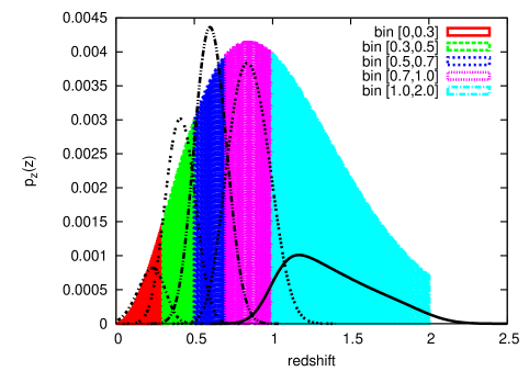
Figure 1: Assumed redshift distribution of galaxies and redshift binning for the fiducial lensing survey. Shadowed areas highlight the sample selections in the distribution of redshift estimates, and the black lines show the true redshift distribution within the samples after including the effect of a redshift uncertainty of $\sigma_{z}=0.05(1+z)$. As additional survey parameters, we have $\bar{n}=30\,\rm arcmin^{-2}$ (sources) and $\bar{n}=3\,\rm arcmin^{-2}$ (lenses), an effective survey area of $200\,\rm deg^{2}$, and a shape noise variance $\sigma_{\epsilon}=0.3$. All galaxies are unbiased with respect to the dark matter density field.

We now move on to quantifying the accuracy of the estimators in Eqs. (20), (31), and (39) for prospective lensing surveys. For this purpose, we assume an effective fiducial survey area of $200\,\rm deg^{2}$ in which galaxies, sources, and lenses have a frequency distribution $p_{z}(z){\rm d}z$ in redshift given by (Baugh & Efstathiou, 1994)

$$p_{z}(z)\propto z^{\alpha}{\rm e}^{-(z/z_{0})^{\beta}}\;,$$ (41)

where $z_{0}=0.7$, $\alpha=2.0$, and $\beta=1.5$, and the mean redshift is hence $\bar{z}=0.9$. To account for the impact of redshift errors, the redshifts in this distribution are assumed to be estimates, such as photometric redshifts based on the photometric filter system of the survey. The estimates are unbiased with an assumed Gaussian root mean square (r.m.s.) uncertainty of $\sigma_{z}=0.05(1+z)$, which is similar to contemporary accuracy levels (Hildebrandt et al., 2008). The total mean number density of sources is set to $\bar{n}=30\,\rm arcmin^{-2}$. The intrinsic shape noise of the sources has an r.m.s. variance of $\sigma_{\epsilon}=0.3$ for each ellipticity component. Hence, the given survey parameters are quite optimistic in terms of the galaxy number density and survey depth, reflecting typical parameters of a presumably space-based survey.

Lenses constitute only ten percent of the total number of sources, that are randomly chosen from the total source sample. The idea is that in reality we select a subpopulation of lens galaxies to be studied, rather than the maximum number of galaxies. In the mock data, lenses still, however, have the same $z$-distribution as sources. In this scenario, galaxies are unbiased with respect to the dark matter distribution, i.e., $b(k,\chi)=r(k,\chi)=1$ for all scales $k$ and radial distances $\chi$.

For the mock analysis, the galaxy sample is split into $N_{\rm lens}=N_{\rm source}=5$ (photometric) redshift bins $[0,0.3],[0.3,0.5],[0.5,0.7],[0.7,1],[1,2]$ with no overlap. The last redshift bin is relatively broad, as we do not expect to obtain very accurate redshift estimates for galaxies with $z\in[1,2]$. The distribution inside the redshift slices is convolved with the Gaussian redshift uncertainty $\sigma_{z}$ to obtain the true redshift distributions. Owing to the uncertainty in the redshift estimators, distributions of different samples subsequently overlap in the radial direction. The analysis assumes that the resulting true distributions are precisely known. The redshift binning and distribution of galaxies is illustrated by Fig. 1.

The grid defining the band boundaries of the three power spectra $P_{\delta}(k,\chi)$, $P_{\delta\rm g}(k,\chi)$, and $P_{\rm g}(k,\chi)$ is defined by the ranges $k\in[0.01\,h\,{\rm Mpc^{-1}},50\,h\,{\rm Mpc^{-1}}]$ with $N_{k}=10$ log-bins and $z\in[0,2]$ for $N_{z}=5$ redshift bins. The redshift bins for the grid are identical to the bins of the angular correlation functions. In generally, the grid redshift limits could be chosen independently, and the number of redshift bins might also differ. For the fiducial 3D matter power spectrum, we adopt the fitting formula of Smith et al. (2003). Matter and galaxies cluster exactly as in the reference matter power spectrum, i.e., all $f_{mn}=1$.

2.5 Measurement noise

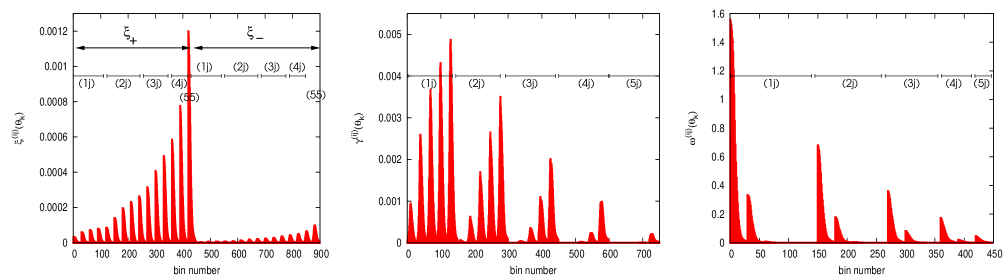
Figure 2: Noise-free data vectors $\@vec{\xi}$ (left), $\@vec{\overline{\gamma}}_{\rm t}$ (middle) and $\@vec{\omega}$ (right). Used are $N_{\rm source}=5$ source redshift slices and $N_{\rm lens}=5$ lens redshift slices; $i,j$ are indices of slices sorted by ascending mean redshift. The data vector elements are sorted by tomography index $(ij)$ and then angular separation, $N_{\theta}=30$. A spike corresponds to one $(ij)$ tomography block with varying $\theta$.

The essential ingredients for quantifying the estimators’ accuracy are the noise covariances ${\@tens{N}}_{\xi}$ (shear-shear correlations), ${\@tens{N}}_{\gamma}$ (galaxy-galaxy lensing), and ${\@tens{N}}_{\omega}$ (lens clustering). This includes the source shape noise, lens position shot-noise, and cosmic variance of the actual signal. For an extensive discussion of the noise terms in $\xi_{\pm}$ we refer to for example Schneider et al. (2002). Towards this goal, we make $N_{\rm real}=4800$ realisations of mock shear and lens catalogues in $2\times 2\,\rm deg^{2}$ fields based on the previous survey parameters and the matter/galaxy clustering in our fiducial cosmological model; shear fields are Gaussian random fields and galaxy number density fields obey log-normal statistics. The details of the mock catalogue generation are laid out in Appendix B. Each mock survey field is processed to estimate the cosmic shear correlations $\xi_{\pm}^{(ij)}(\theta)$ (Schneider et al., 2002), the galaxy-galaxy lensing signal $\overline{\gamma}_{t}^{(ij)}(\theta)$ (e.g., Simon et al., 2007) and the lens clustering $\omega^{(ij)}(\theta)$ (Landy & Szalay, 1993). The correlators are hence estimated exactly as in a real analysis; references for the employed estimators are given inside the previous brackets. The correlation functions are estimated between angular separations of $\theta\in[3^{\prime\prime},2\,\rm deg]$ using $N_{\theta}=30$ log-bins. The tomography measurements for all three correlators are separately combined into a data vector $\@vec{d}_{i}$ for each realisation $i=1\ldots N_{\rm real}$. The data vectors have the following structure:

• $\xi_{\pm}^{(ij)}(\theta)$: The first half of $\@vec{d}_{i}$ contains estimates of $\xi_{+}$, whereas the second half contains the $\xi_{-}$ measurements. Both the $\xi_{+}$ and $\xi_{-}$ values are sorted as tomography blocks of constant index $(ij)$ and ascending index $i$, $i\leq j$. Within a block, values are arranged in order of increasing angular separation bin $\theta_{l}$. Since there are $N_{\theta}$ angular bins, $N_{\rm source}(N_{\rm source}+1)/2$ tomography blocks, and two correlation functions, the data vector realisations $\@vec{d}_{i}$ have in total $N_{\theta}N_{\rm source}(N_{\rm source}+1)=900$ elements.

• $\overline{\gamma}_{\rm t}^{(ij)}(\theta)$: Likewise, GGL measurements are sorted in order of tomography block $(ij)$ index with ascending lens sample index $i$ and source sample index $j$. All $(ij)$ combinations are allowed, i.e., $N_{\rm lens}N_{\rm source}$ combinations. Inside a block, values are ordered by increasing lens-source angular separation. This yields in total $N_{\theta}N_{\rm lens}N_{\rm source}=750$ elements.

• $\omega^{(ij)}(\theta)$: Measurements of the angular lens clustering are again sorted in order of tomography bin index $(ij)$ with $i\leq j$ and $i,j$ being the lens sample indices; there are in total $N_{\rm lens}(N_{\rm lens}+1)/2$ block combinations. Inside a block, measurements are sorted in order of increasing lens-lens separation. In total, this yields $N_{\theta}N_{\rm lens}(N_{\rm lens}+1)/2=450$ elements.

Noise-free data vectors with fiducial survey parameters are depicted in Fig. 2.

As an estimator of the noise covariance based on the mock data realisations, we devise the field-to-field variance

$${\@tens{C}}_{\rm est}=\frac{1}{N_{\rm real}-1}\sum_{i=1}^{N_{\rm real}}\left(\@vec{d}_{i}-\overline{\@vec{d}}\right)\left(\@vec{d}_{i}-\overline{\@vec{d}}\right)^{\rm t}\;,$$ (42)

where

$$\overline{\@vec{d}}=\frac{1}{N_{\rm real}}\sum_{i=1}^{N_{\rm real}}\@vec{d}_{i}$$ (43)

is the ensemble mean. The resulting matrix ${\@tens{C}}_{\rm est}$ estimates the noise covariance ${\@tens{N}}_{\xi}$, ${\@tens{N}}_{\gamma}$, or ${\@tens{N}}_{\omega}$ in a $A_{4}=2\times 2\,\rm deg^{2}$ survey depending on whether $\@vec{d}_{i}$ consists of $\xi_{\pm}^{(ij)}(\theta)$, $\overline{\gamma}_{\rm t}^{(ij)}(\theta)$, or $\omega^{(ij)}(\theta)$, respectively. We scale this to the expected noise in a larger $A_{200}=200\,\rm deg^{2}$ survey by multiplying ${\@tens{C}}_{\rm est}$ with $A_{4}/A_{200}=1/50$. This mimics a survey of area $A_{200}$ consisting of 50 statistically independent patches of size $A_{4}$ each. Finally, since the band power estimators require the inverse noise covariance, we utilise the inverse covariance estimator of Hartlap et al. (2007), which is based upon ${\@tens{C}}^{-1}_{\rm est}$.

For the covariance estimation and the mock analysis, lenses are a randomly chosen subsample of the sources (ten percent). In particular, sources are clustered as the projected dark matter distribution up to the level of the Poisson shot noise. The choice of identical redshift bins for lenses and sources is due purely to the means by which the mock survey galaxy catalogues are generated. In the estimator formalism, lenses and sources may have different radial distributions and the number of subsamples may differ as well. The $z$-slices in the mock data overlap due to the adopted redshift uncertainty. Therefore, we have a non-vanishing $\omega^{(ij)}(\theta)$ for $i\neq j$, which can be seen in the right panel of Fig. 2.

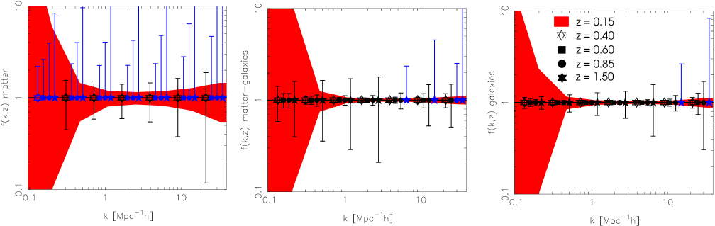
Figure 3: A simulated reconstruction of the 3D band matter power spectrum $P_{\delta}(k,\chi)$ (left), galaxy-matter cross-correlation power spectrum $P_{\delta\rm g}(k,\chi)$ (middle), and galaxy power spectrum $P_{\rm g}(k,\chi)$ (right) utilising the minimum variance estimators in Sect. 2. Shown are the average estimated band powers $f_{mn}$ relative to the fiducial band power spectrum. The shadowed area in the background indicates the $68\%$ confidence region of the lowest redshift bin $\bar{z}=0.15$. The data points denote estimates at higher redshifts. The error regions indicate the $1\sigma$ uncertainties of the estimators via Eq. (22), (32), or (40). Data points in blue colour or with asymmetric error bars indicate estimates that are consistent with zero. Note that data points within the same $k$-bin are slightly shifted with respect to each other along the $k$-axis for clarity.

2.6 Forecasts

Using the fiducial survey and the predicted measurement noise, constraints on the three power spectra are shown in Fig. 3. The figures are obtained by applying the estimators to a noise-free data vector (Fig. 2), whereas the error bars are based on estimates of the measurement noise in the mock survey, that is either Eq. (22), (32), or (40). The data points or the centre of the shadowed region therefore simulate the statistical average of a band power estimation process for an infinite number of similar surveys. The error bars or regions, however, are the predicted $1\sigma$ uncertainties in a typical single $200\,\rm deg^{2}$ survey. As can be seen, the average data points lie exactly on $f_{\rm mn}=1$, indicating that they were evaluated with an unbiased estimator.

In general, the constraints involving cosmic shear become worse with increasing redshift owing to the decreasing number of background sources at higher redshifts. For the matter power $f_{\delta,mn}$, we find only upper limits in the redshift bins $z>0.5$ or for scales $k\lesssim 0.3\,h\rm Mpc^{-1}$, but reasonable constraints for $z\lesssim 0.4$ and $0.5\leq k\,h^{-1}{\rm Mpc}\leq 10$. A similar conclusion can be drawn for $f_{{\delta\rm g},mn}$, albeit the constraints are here considerably improved, especially at higher redshift. Under our assumptions, the galaxy band power spectrum of the lenses, $f_{{\rm g},mn}$, is extremely well-recovered. The detection fidelity depends mainly on the number of lenses within a redshift bin. In reality, this number is likely to be even smaller as in the mock survey, depending on the galaxy population selected for investigation (see, e.g., Zehavi et al., 2011).

Since the correlation functions cover only a certain angular range, we may anticipate obtaining biased estimates for large-scale modes $k$. This bias can be quantified by utilising both Eq. (23) for $\@vec{f}^{\rm ref}_{\delta}$ and equivalent bias indicators for the two other band powers $\hat{\@vec{f}}_{\delta\rm g}$ and $\hat{\@vec{f}}_{\rm g}$. For the band limits and fiducial power spectrum chosen, the bias is smaller than 0.1 percent and therefore no concern to us here. We note, however, that a bias clearly becomes visible for $P^{\rm fid}_{\delta}(k,\chi)\equiv 1$ and $k\lesssim 0.2\,h\rm Mpc^{-1}$. Therefore, a realistic matter power spectrum when used as a reference aids the stability of the minimum variance estimators.

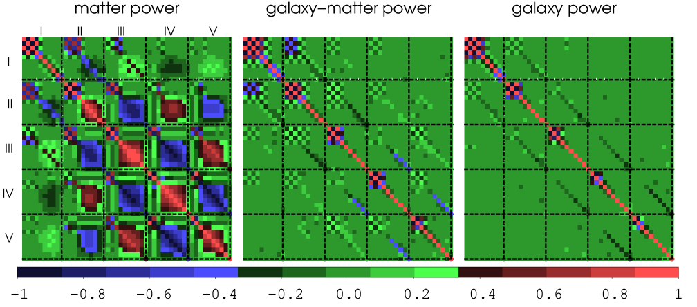
Figure 4: Correlation matrix of uncertainties in the relative band powers (minimum variance estimators). Roman numbers indicate the redshift bins ($\bar{z}=0.15,0.4,0.6,0.85,1.5$ for I-V, respectively). Within blocks, highlighted by dashed lines, the correlation between $k$-bins of either identical $z$-bins (diagonal blocks) or different $z$-bins (off-diagonal blocks) is plotted. The mean wave numbers of the $k$-bins are $\bar{k}=0.01,0.02,0.05,0.13,0.30,0.71,1.66,3.88,9.10,21.33$ in units of $h\,\rm Mpc^{-1}$.

The correlation of the estimator uncertainties are depicted in Fig. 4. Uncertainties in the estimates of the relative band powers $f_{\delta,mn}$ clearly become increasingly correlated at higher redshift. Most independent estimates are located in the lowest redshift bin, where the constraints are also tightest (Fig. 3). For $z>0.4$, the errors evidently become strongly correlated because all shear-shear correlation functions are sensitive to the same matter density fluctuations in front of the sources: For constant $k$, $f_{\delta,mn}$ adjacent in redshift are anti-correlated. For neighbouring bands in the same redshift bin, errors are also strongly correlated for $z>0.4$. Therefore, there is little statistically independent information in the $f_{\delta,mn}$ at higher redshift. The correlation of errors becomes small for the galaxy-matter band power $f_{{\delta\rm g},mn}$ and is almost absent for the galaxy band power $f_{{\rm g},mn}$. However, all estimates still exhibit strong correlations between adjacent $k$-bins in the large-scale regime (small $k$) because the bins are associated with density modes that are barely touched by the angular correlation functions of limited angular range.

3 Bayesian analysis

The minimum variance estimators of the foregoing section are quick and easy to apply to the data. Moreover, their statistical errors are equally straightforward to assess. However, they have the disadvantage that band power estimates can also become negative for the auto-correlation power spectra $P_{\delta}(k,\chi)$ and $P_{\rm g}(k,\chi)$, which by their definitions is not allowed. One frequently finds band power estimates oscillating about zero where errors are large. Therefore, the question arises of whether one can refine the analysis to explicitly incorporate non-negative powers. This refinement may also help to improve the recovery of the matter power spectrum, which in the foregoing minimum variance analysis was only successful at low redshifts, where the majority of band power factors $f_{\delta,mn}$ had only upper limits. We note that the cross-correlation power $P_{\delta\rm g}(k,\chi)$ can in principle become negative, if the galaxy correlation parameter $r(k,\chi)$ is negative.

3.1 Method

A refinement can be achieved in the framework of a Bayesian analysis (cf. MacKay, 2003), where we determine the posterior likelihood

$$p\big{(}\@vec{m}|\@vec{d}\big{)}\propto{\cal L}\big{(}\@vec{d},\@vec{m}\big{)}\times p_{\rm prior}\big{(}\@vec{m}\big{)}$$ (44)

of our model parameters $\@vec{m}$ – for instance, the band power values $\@vec{f}_{\delta}$ in the case of $P_{\delta}(k,\chi)$ – for the observed tomography correlation functions $\@vec{d}$, which is $\@vec{\xi}$ for the example mentioned; ${\cal L}(\@vec{d},\@vec{m})$ is the data likelihood function and $p_{\rm prior}(\@vec{m})$ the a-priori information on the band power (prior).

In the case of $\@vec{f}_{\delta}$, we solely assume a prior that enforces positive or zero band powers

$$p_{\rm prior}\big{(}\@vec{f}_{\delta}\big{)}=\prod_{n=1}^{N_{z}}\prod_{m=1}^{N_{k}}H\big{(}f_{\delta,mn}\big{)}\;,$$ (45)

where $H(x)$ is the Heaviside function of $x$. A conceivable modification of the prior could consist of including available empirical information on the matter power spectrum. For the likelihood function, we presume Gaussian noise

$${\cal L}_{\xi}\big{(}\@vec{\xi},\@vec{f}_{\delta}\big{)}\propto\exp{\left(-\frac{1}{2}\left[\@vec{\xi}-{\@tens{X}}\@vec{f}_{\delta}-\@vec{\xi}_{\rm fid}\right]^{\rm t}{\@tens{N}}_{\xi}^{-1}\left[\@vec{\xi}-{\@tens{X}}\@vec{f}_{\delta}-\@vec{\xi}_{\rm fid}\right]\right)}\;,$$ (46)

with a constant noise covariance ${\@tens{N}}_{\xi}$ that does not depend on the matter power spectrum. The likelihood functions ${\cal L}_{\gamma}$ and ${\cal L}_{\omega}$ for $\@vec{f}_{\delta\rm g}$ and $\@vec{f}_{\rm g}$, respectively, are defined accordingly. Furthermore, for $f_{{\rm g},mn}$ we employ a prior similar to the $f_{\delta,mn}$ prior, but allow $f_{{\delta\rm g},mn}$ to be negative (negative correlations).

Another convenience of the Bayesian approach is that one can easily accommodate a transformation of model parameters in the analysis, yielding the statistics of an alternative parameter set. We take advantage of this by also determining the posterior likelihoods of band galaxy biasing parameters $(b_{mn},r_{mn})$ by expressing $\@vec{f}_{\delta\rm g}$ and $\@vec{f}_{\rm g}$ as

$$f_{{\delta\rm g},mn} = r_{mn}b_{mn}\,f_{\delta,mn}\;,$$ (47)

$$f_{{\rm g},mn} = b^{2}_{mn}\,f_{\delta,mn}\;,$$

for all $m=1\ldots N_{k}$ and $n=1\ldots N_{z}$. Here the prior ensures that the bias factors $b_{mn}$ and the relative band powers $f_{\delta,m}$ are positive, thereby directly constraining $b(k,\chi)$ and $r(k,\chi)$, provided that we employ the same reference fiducial power spectrum for the matter, galaxy-matter, and galaxy power spectrum. In this variant, we combine the information on all $(f_{\delta,mn},f_{{\delta\rm g},mn},f_{{\rm g},mn})$ to constrain the biasing parameters. Consequently, we now have a combined posterior likelihood instead of the three separate ones in the previous case

$$p\big{(}\@vec{f}_{\delta},\@vec{b},\@vec{r}|\@vec{d}\big{)}\propto p_{\rm prior}\big{(}\@vec{r},\@vec{b},\@vec{f}_{\delta}\big{)}\,\times$$

$${\cal L}_{\xi}\big{(}\@vec{\xi},\@vec{f}_{\delta}\big{)}{\cal L}_{\gamma}\big{(}\@vec{\overline{\gamma}}_{\rm t},\@vec{f}_{\delta\rm g}=\@vec{br}\@vec{f}_{\delta}\big{)}{\cal L}_{\omega}\big{(}\@vec{\omega},\@vec{f}_{\rm g}=\@vec{b}^{2}\@vec{f}_{\delta}\big{)}\;.$$

We assume that noise correlations between $\xi_{\pm}$, $\overline{\gamma}_{\rm t}$, and $\omega$ estimators are negligible, hence likelihood function factors are combined as shown, where $(\@vec{b},\@vec{r})$ denotes the biasing parameters and $(\@vec{brf}_{\delta},\@vec{b^{2}f}_{\delta})$ provide an abbreviated version of Eq. (47).

We sample the posterior likelihoods numerically by devising the Markov chain Monte Carlo (MCMC) technique (e.g., MacKay, 2003), where the noise covariances of the minimum variance estimators $\hat{\@vec{f}}$ are used as yardsticks to set up the proposal function for the Metropolis-Hastings algorithm.

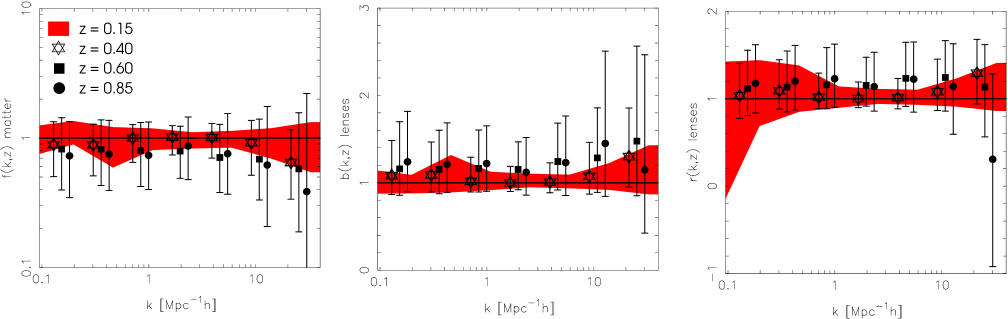
Figure 5: Bayesian MCMC analysis of the fiducial survey estimating the matter band power (left; relative to the fiducial power spectrum) and the galaxy biasing parameters (middle: bias factor; right: correlation factor). The shadowed area in the background highlights a $68\%$ credibility region about the marginalised posterior mean for the lowest redshift bin $\bar{z}=0.15$, whereas data points delineate the $68\%$ credibility regions about the mean at higher redshifts. The highest, most poorly constrained redshift bin is not included here. The results are subject to some numerical noise caused by the adopted MCMC technique.

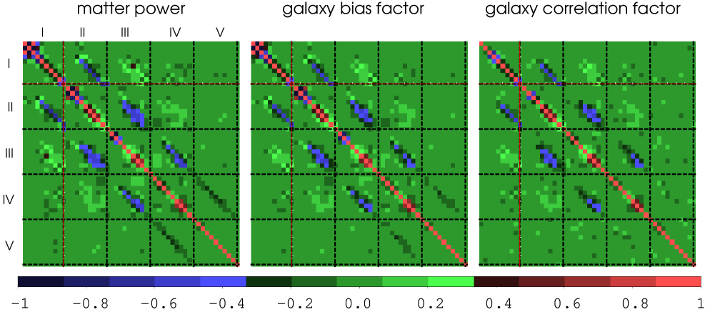
Figure 6: Correlation matrix of band power and galaxy biasing parameter estimates in the Bayesian framework (see Fig. 5). See caption of Fig. 4 for more information.

3.2 Forecasts

Fig. 5 shows the constraints on the fiducial survey (Sect 2.4) obtained via the Bayesian analysis. We show only the variant that uses biasing parameters to express the galaxy-matter and galaxy power spectrum. As before with the minimum variance estimators, the constraints are obtained by using a noise-free data vector as input data, as shown in Fig. 2. The likelihood functions ${\cal L}_{\xi,\gamma,\omega}$ assume a level of noise that is similar to that in the $200\,\rm deg^{2}$ fiducial survey. This combination basically simulates the typical posterior of a $200\,\rm deg^{2}$ survey. We plot the means of the marginalised one-dimensional (1D) posteriors of $(f_{\delta,mn},b_{mn},r_{mn})$ and the r.m.s. variance in their MCMC values above (upper error bars) or below the mean (lower error bars). This defines a 68 percent credibility region for every parameter. The prior is defined to constrain the galaxy biasing parameters a priori for $b(k,\chi)\in[0,4]$ and $r(k,\chi)\in[-2,2]$ (flat priors). These priors broadly delineate the regime that is expected for galaxy bias (e.g. Guzik & Seljak, 2001; Seljak et al., 2005).

We note that owing to the subtraction of Poisson shot noise in the definition of $P_{\rm g}(k,\chi)$ (Eq. 5), the modulus of the correlation coefficient $r$ can be larger than unity. A value of $|r|>1$ indicates a discrete galaxy sampling that differs from a Poisson process as, for instance, predicted on small scales in the halo model (cf. Guzik & Seljak, 2001). The Monte Carlo mock data employed in this study uses an explicit Poisson process to generate galaxy positions out of a smooth number density field (Appendix).

For $\@vec{f}_{\delta}$, a flat prior on a logarithmic-scale was used. However, we found that a prior flat on a linear scale yields similar results for $\@vec{f}_{\delta}$ in our case. This result, which is based on a noise-free data vector, shows that the mean of the 1D posterior probability distribution function (p.d.f.) is not an unbiased estimator of any $f_{mn}$, but the mean is biased to too low values for $f_{\delta,mn}$ and biased too high for $b_{mn}$ and for most factors $r_{mn}$. This result also depends on the adopted priors, particularly when the constraints from the data are weak. For example, the flat prior for $b_{mn}$ tends to predict values of $b_{mn}$ of around two. We note, however, that here the true $f_{mn}=1$ always falls into the above defined 68 percent credibility region such that the bias appears to be at least smaller than the r.m.s. uncertainty caused by measurement noise. This can be explained in the following way. First, the posterior mean $\langle f_{mn}\rangle$ is an optimal estimator $f^{\rm est}_{mn}$ in the sense that it minimises the average estimator error

$$\Big{\langle}\Delta^{2}f_{mn}^{\rm est}\Big{\rangle}:=\int{\rm d}f_{mn}\,p\big{(}f_{mn}|\@vec{d}\big{)}\,\left(f_{mn}^{\rm est}-f_{mn}\right)^{2}$$ (49)

as to the true $f_{mn}$ with posterior $p(f_{mn}|\@vec{d})$ because

$$\frac{{\rm d}\langle\Delta^{2}f_{mn}^{\rm est}\rangle}{{\rm d}f^{\rm est}_{mn}}=0\leavevmode\nobreak\ {\rm for}\leavevmode\nobreak\ f^{\rm est}_{mn}\equiv\langle f_{mn}\rangle=\int{\rm d}f_{mn}\,p(f_{mn}|\@vec{d})\,f_{mn}\;.$$ (50)

Second, the average error when adopting $f^{\rm est}_{mn}=\langle f_{mn}\rangle$ is simply the r.m.s. variance in the posterior, as can be seen by substituting $\langle f_{mn}\rangle$ for $f^{\rm est}_{mn}$ in Eq. (49).

As with the minimum variance estimators, the strongest constraints are found for the regime $0.5\lesssim k\,h^{-1}\,{\rm Mpc}\lesssim 10$. The constraints on the band matter power spectrum, for which we had upper limits only for the minimum variance estimates, are clearly improved by the assertion of positive auto-power spectra. We note the apparent strong improvement for $k\lesssim 0.5\,h\rm Mpc^{-1}$, which is merely a combined effect of the priors on $f_{\delta,mn}$ and the bias factor and, possibly, also the information on the galaxy clustering on large scales from the data.

In addition, the MCMC results are devised to estimate the correlation of the errors as a correlation matrix in Fig. 6. This also shows an improvement for $f_{\delta,mn}$. The correlation of errors is softened, hence much less pronounced than in Fig. 4, although we can still make out the anti-correlation among the bins that are adjacent in redshift. The (band) galaxy bias and correlation factors $b_{mn}$ and $r_{mn}$ have errors that are very similar to those of $f_{\delta,mn}$ since the correlation pattern of the latter is imprinted in the galaxy biasing parameters owing to the mixing of $f_{\delta,mn}$, $f_{{\delta\rm g},mn}$, and $f_{{\rm g},mn}$ within the Bayesian analysis.

4 Discussion and conclusions

This paper has presented methods for constraining from tomography data the deprojected power spectra of the matter clustering and the related clustering of galaxies. Moreover, a fiducial survey has been employed to determine the prospects for the application of this method to real data.

The prerequisite for a successful application of this technique is the availability of radial (redshift) information for survey galaxies, which will be provided by ongoing lensing surveys and surveys in the near future. On the basis of this radial information, sources and lenses can be divided into subsamples with known radial distributions, which are disjunct slices in the optimal case, thereby probing matter and galaxy clustering at different effective redshifts and on different physical scales. From the cosmic shear tomography alone, the spatial matter power spectrum can be measured, which represents an advance on older lensing methodologies (Schneider et al., 2002; Pen et al., 2003; Bacon et al., 2005). Augmenting this with measurements of galaxy-galaxy lensing and angular lens clustering for all pair combinations of galaxy subsamples, constraints on the galaxy biasing can also be made as a function of redshift and length-scale. This improves older non-parametric lensing techniques for probing galaxy biasing (Schneider, 1998; van Waerbeke, 1998) since tomography correlations can be directly traced back to the underlying 3D power spectrum. In particular, the calibrations of bias parameters due to projection effects developed by Hoekstra et al. (2002) are no longer required. This promises to provide a simplified comparison to theoretical galaxy or dark matter models (cf. Yoshikawa et al., 2001; Weinberg et al., 2004; Springel et al., 2005).

4.1 Methodology

We have shown in this paper that by approximating the 3D power spectra by band power spectra relative to a fiducial band power spectrum, there is a straightforward linear relation between the observable angular correlation functions (shear-shear correlations, mean tangential shear about lenses, and lens clustering) and the 3D power spectra (matter power, matter-galaxy cross power, and galaxy power), where Limber’s approximation applies. This study proposed two approaches to inverting this linear relation in a statistical way:

• The first approach makes use of minimum variance estimators that provide estimates of the relative 3D band powers. The approach is similar to that of Pen et al. (2003), but now permits the full amount of tomography information to be used. By doing so we can now, therefore, observe the time-evolving power spectra rather than the average power at an effective depth of the survey. Furthermore, by choosing a theoretical power spectrum as reference, the minimum variance estimators allow us to compare a theoretical band power directly to the data. Differences between the theory and data are thereby revealed by a relative band power significantly $f_{\rm mn}\neq 1$.

• The second approach is a full Bayesian analysis for which we can, in addition, express the galaxy-matter and galaxy power spectrum in terms of the linear galaxy biasing functions $b(k,\chi)$ and $r(k,\chi)$. The biasing functions are related to the angular correlation functions in a nonlinear fashion. The Bayesian framework automatically accounts for this nonlinearity in the posterior likelihood of the biasing parameters, being the output of the analysis. Moreover, we can easily implement the prior knowledge that the matter and galaxy power, by definition variances, have to be positive or zero. On the other hand, the disadvantage of the Bayesian approach is that we have to specify the complete noise statistics of the measurements, whereas the minimum variance estimators formally only require the noise covariances. For the scope of this paper, we adopted a multivariate Gaussian noise model. This does not exactly hold true (Schneider & Hartlap, 2009; Keitel & Schneider, 2011), but a more sophisticated noise model can be built into the analysis by modifying the likelihood function in Eq. (46) in future applications. Moreover, the Bayesian framework also allows us to add prior information about the matter power or galaxy biasing from other observations.

Both approaches rely on a known angular diameter distance, $f_{\rm k}(\chi)$, in addition to a specified relation between radial comoving distance $\chi$ and redshift for a given fiducial cosmology model. Although this may sound like a strong restriction, those geometric properties of the Universe are known to great accuracy and are consistently inferred by a wide range of observations (e.g., Komatsu et al., 2011). The nonlinear structure of matter at $z\lesssim 1$, on the other hand, is prone to a larger uncertainty as discussed, for instance, by van Daalen et al. (2011).

4.2 Mock survey

To estimate the performance of the estimators, we assumed a fiducial survey with a $200\,\rm deg^{2}$ area, a mean galaxy redshift of $\bar{z}=0.9$, reaching as deep as $z=2.0$ for usable redshift estimates, and a source number density of $\bar{n}=30\,\rm arcmin^{-2}$ (Sect. 2.4 for more details). Lenses are a subsample of ten percent of the source catalogue, but have an identical $z$-distribution. This is because a smaller galaxy population is usually studied as lenses. We assumed that the angular correlation functions can safely be measured between 3 arcsec and $2$ degree. Separations much smaller than 3 arcsec will be difficult to measure owing to the apparent size of smeared galaxy images or the pixel size in the instruments. Separations larger than $\sim 2$ degree are principally possible, but this would extend into a regime where the flat-sky approximation, used for the formalism of this paper, would begin to fail. This may be remedied by a full-sky treatment comparable to Castro et al. (2005).

The fiducial parameters were chosen to be somewhere in-between typical figures of current or near future surveys. The assumed survey depth is, however, probably more on the side of deeper space-based lensing surveys such as COSMOS or the upcoming Euclid mission, rather than on the side of shallower ground-based surveys such as CFHTLS, KiDS, or Pan-STARRS. On the other hand, the adopted number density of sources is smaller than expected for a spaced-based mission but still higher than the typical number density achieved in ground-based surveys ($\sim 10\,\rm arcmin^{-2}$). Moreover, the modest fiducial survey area of $200\,\rm deg^{2}$ reflects the order-of-magnitude for a contemporary ground-based lensing survey, that is capable of delivering cosmic shear data such as the CFHTLS. In the not too distant future, this figure is likely to be increased by another order of magnitude.

4.3 Simulated noise covariance

The predicted noise covariance of the correlation functions was derived from realisations of mock surveys (Appendix B). In analogy to the Monte Carlo method put forward in Simon et al. (2004), I included a new feature to account for the clustering of galaxies, obeying a log-normal statistics, and to include a mock galaxy-galaxy lensing signal. This approach is imperfect in several respects:

• The assumption of Gaussian statistics for the cosmic shear fields is inaccurate for nonlinear scales (roughly ten arcmin or smaller), which leads to an underestimation of the shear noise covariance (Semboloni et al., 2007; Hartlap et al., 2009; Hilbert et al., 2011). The adopted log-normal statistics (Bouchet et al., 1993) of the galaxy clustering, on the other hand, is presumably a good approximation of the galaxy-galaxy lensing and galaxy clustering covariance.

• As realisations on grids are performed (grid sizes are $4\times 4\,\rm deg^{2}$ from which the smaller patches are cropped), we miss angular modes on scales larger than $\gtrsim 4\,\rm deg$ (Simon et al., 2004). Computation time constraints in our approach do not allow much larger fields with more galaxies.

• The covariance is estimated on a patch-by-patch basis, which assumes a discontinuous, patchy survey rather than a contiguous survey area where galaxy pairs across patches could also be used to estimate the angular correlation functions. This reduces the effective number of galaxy pairs and yields more noise than for a realistic contiguous survey area.

Although the last effect presumably partly compensates for the two others, we should expect an overly optimistic noise covariance and hence possibly overly optimistic constraints on the band power spectra. In the future, a more accurate estimate could be obtained by ray-tracing through cosmological structure formation simulations (White & Hu, 2000; Hilbert et al., 2009; Kiessling et al., 2011; Li et al., 2011). As the noise covariances for the tomography correlators are necessarily large in size (Fig. 2 for bin numbers), however, a large number of statistically independent realisations would be required (this paper uses 4800 realisations, thus in total $19200\,\rm deg^{2}$) to properly estimate the inverse noise covariance (Hartlap et al., 2007).

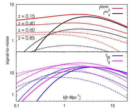
Figure 7: Predicted signal-to-noise ratio of the relative band powers $f_{mn}$ for different redshift bins (see key for line styles in the top panel). Minimum variance estimators and Bayesian analysis give comparable results except for the matter band power $f_{\delta,mn}$ (top panel), which here combines constraints from lensing and galaxy clustering with priors $b\leq 4$ and $|r|\leq 2$ in the Bayesian approach. The bottom panels shows the signal-to-noise of the minimum variance estimates.

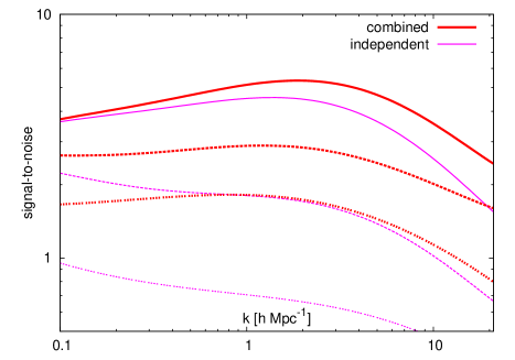
Figure 8: Signal-to-noise ratio per band of the reconstructed matter power spectrum $f_{\delta,mn}$ in a Bayesian analysis, either for an analysis of the shear tomography alone (“independent”), or when combining galaxy clustering, lensing with priors $b\leq 4$, $|r|\leq 2$ (“combined”). Plotted are the three first redshift bins $\bar{z}=0.15,0.4,0.6$ (top to bottom line).

4.4 Reconstructed band powers

The fiducial survey predictions are summarised by Figs. 3 and 5 for the minimum variance and Bayesian approach, respectively. The latter does not include the highest redshift bin, $\bar{z}=1.5$, because of its poor constraints. Figs. 4 and 6 visualise the correlation of errors in the estimates. The correlation of errors is quite strong for $f_{\delta,mn}$, but considerably weaker for $f_{{\delta\rm g},mn}$ and $f_{{\rm g},mn}$ (similar between the minimum variance and Bayesian technique). Compared to the minimum variance estimator, the Bayesian analysis eases the strong correlation of errors in the matter band power spectrum,.

We adopted $N_{z}=5$ redshift bins and $N_{k}=10$ k-bins on a logarithmic-scale. The MCMC algorithm is well-suited to fitting many free model parameters simultaneously (here $N_{k}N_{z}=50$), but converges slower if their number becomes larger. For this reason, a small number of bins is desirable. Because adjacent bands are already moderately to strongly correlated in the $k$- or $z$-direction, especially for $f_{\delta,mn}$, a much finer binning than the one adopted is probably not necessary, although this should be quantified in an objective way for future applications. A principal component analysis (e.g., Tegmark et al., 1997), based on the minimum variance estimator noise, could be employed to identify the most significant modes in the $(k,z)$-plane and find an optimised representation of the power spectra for the Bayesian analysis. Two interesting binning extremes are conceivable:

• On the one hand, we could use $N_{k}=1$ and a larger number of redshift bins. Using a fiducial 3D power spectrum with a reasonably realistic shape but normalised at all redshifts to the variance in the local Universe, we could focus on the overall growth of the fluctuations from the tomography data alone. This would result in an analysis similar to the one in Bacon et al. (2005).

• On the other hand, we could use $N_{z}=1$ and a larger number of $k$-bins. If the time evolution of the structure growth is realistically built into the fiducial power spectrum, then the methodology from this paper would infer the deviation from the fiducial power as a function of scale averaged over the full redshift range. This would focus on deviations from the shape of the theoretical power spectrum, taking the expected structure growth out of the equation.

As long as estimates are very noisy – auto-correlation band powers are consistent with zero in the minimum variance approach – the Bayesian approach provides tighter constraints (Fig. 7). Both approaches are otherwise comparable. The signal-to-noise ratio in the Bayesian analysis equals the mean of the marginalised posterior divided by the variance about the mean. On large scales $k\lesssim 1\,h\rm Mpc^{-1}$, however, the signal-to-noise does not fall off as quickly as for the minimum variance estimators: it forms instead a plateau. By performing a Bayesian analysis for the matter power spectrum combined with galaxy clustering and one analysis based on shear tomography alone, we have found that the plateau is the result of the asserted positive power $P_{\delta}(k,\chi)\geq 0$ (“independent” lines in Fig. 8) rather than the effect of adding galaxy clustering information and the upper limits to $b$ and $r$ (“combined”).

We expect, on average, the signal-to-noise to decrease with redshift, although there are more complicated trends on large scales (small $k$) for $f_{{\rm g},mn}$ because galaxy samples at higher redshift probe larger scales and their galaxy numbers increase first with redshift followed by a decline beyond $z\sim 0.9$. We have found that the most significantly measured quantities are the galaxy clustering, then the galaxy-matter cross-correlation, and then the matter clustering. In reality, we should expect the significance of the first two to go down, however, if an even smaller population of lenses is studied than in the fiducial survey.

The signal-to-noise of the relative band power $f_{\delta,mn}$ drops below $\sim 2\sigma$ on all scales beyond $z\gtrsim 0.4$ so that we should not expect strong constraints beyond that redshift. For a survey shallower than the fiducial survey, this limit is bound to decrease yet further. The tightest constraints are obtained for $z\sim 0.2$ and about $k\sim 2h\,\rm Mpc^{-1}$ ($\sim 6\sigma$ detection), away from which the detection fidelity drops relatively quickly below $3\sigma$ for individual bands. In conclusion, for $z\lesssim 0.8$ and comoving $0.5\lesssim k\,h^{-1}\,{\rm Mpc}\lesssim 10$ the 3D band power spectra $f_{{\delta\rm g},mn}$ and $f_{{\rm g},mn}$ can be recovered most effectively, whereas a significant detection of $f_{\delta,mn}$ is restricted to lower redshifts $z\lesssim 0.3$ inside a range $1\lesssim kh^{-1}{\rm Mpc}\lesssim 10$. This is in the heart of the regime discussed in van Daalen et al. (2011), hence an application of lensing tomography promises tom improve our knowledge of the effect of baryons on the matter power spectrum.

As we expect the noise covariances to be overly optimistic, a robust study of the matter power spectrum would, however, probably require coverage of a larger survey area than in our fiducial survey. We can hope for a significant signal enhancement, if the survey area is increased to $\sim 10^{3}\,\rm deg^{2}$ or more, as expected from full-sky surveys. The signal-to-noise should then roughly be boosted by $\sqrt{10}\approx 3.3$ for all band power estimates. Moreover, boosting the number density of sources, for example through space-based surveys, also increases the signal-to-noise as shot-noise on small scales is $\propto\overline{n}^{-1/2}$ (Schneider et al., 2002).

4.5 Reconstructed galaxy biasing parameters

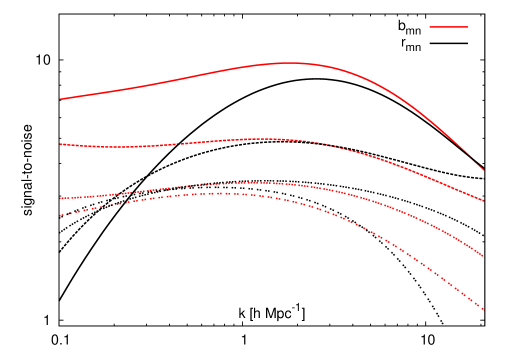
Figure 9: Predicted signal-to-noise of the galaxy biasing parameters $(b_{mn},r_{mn})$ for different redshift bins $\bar{z}=0.15,0.4,0.6,0.85$ (from top to bottom line).

Combining the band power estimates, the Bayesian analysis provides constraints on the galaxy biasing functions (see the two right-hand panels in Fig. 5). Here, the highest accuracy (higher than $\sim 3\sigma$) is achieved for $z\lesssim 0.5$ and $1\lesssim k\,h^{-1}\,{\rm Mpc}\lesssim 10$ (Fig. 9). The detection fidelity clearly depends on the number density of lenses, for which here we assume the fiducial value of $3\,\rm arcmin^{-2}$. An increase in the lens population size will increase the number of galaxy pairs in the estimators for the angular correlation functions and, therefore, reduce measurement noise. Since $P_{\delta\rm g}(k,\chi)$ and $P_{\rm g}(k,\chi)$ are most easily reconstructed, it may be sensible in a survey with poorly confined $P_{\delta}(k,\chi)$ to utilise only those two to constrain $P_{\delta\rm g}/P_{\rm g}\propto r/b$ as a biasing function that can be pinned down with the highest confidence.

The galaxy bias analysis here uses a flat prior with $|r(k,\chi)|\leq 2$ and $b(k,\chi)\leq 4$. The prior has the effect that a highly-significant measurement of galaxy clustering $f_{{\rm g},mn}$ will put a lower limit of $f_{{\rm g},mn}/b_{\rm high}^{2}\leq f_{\delta,mn}$ on the matter clustering, where here $b_{\rm high}=4$. For the same reason, $f_{\delta{\rm g},mn}$ imposes a lower limit of $f_{{\rm g},mn}/(b_{\rm high}r_{\rm high})\leq f_{\delta,mn}$ for $r_{\rm high}=2$ to $f_{\delta,mn}$. Therefore, combining galaxy clustering and shear tomography aids the recovery of the matter power spectrum, as can be seen when comparing “independent” and “combined” lines in Fig. 8. The improvement is mostly present for low signal-to-noise bands in the matter power spectrum. By varying the prior intervals of $b$ and $r$, we found that the improvement is mainly due to the prior of $r$ rather than $b$.

4.6 Systematics

The above predictions rely on the assumption that systematics in the measured correlation functions are negligible. In reality, several potential systematics – unrelated to the data reduction and shape measurements of galaxy images – have been identified and several points can be made:

• Correlations of intrinsic (unlensed) galaxy image shapes (“II”) add to the shear-shear correlation functions $\xi_{\pm}^{(ij)}$ (e.g., Heymans et al., 2006).

• The “GI”-effect is more intricate (Hirata & Seljak, 2004), as it is non-locally produced by correlations between the intrinsic source image shape and the shear effect of its surrounding matter on a more distant source.

• Another unwanted effect that could arise is the influence of cosmic magnification (Narayan, 1989; Bartelmann & Schneider, 2001). Magnification by matter density fluctuations in front of lenses changes the projected number density of lenses; to the lowest order to $\kappa_{\rm g}\mapsto\kappa_{\rm g}+\lambda\kappa$, where $\lambda:=2(\alpha-1)$ and $\overline{N}_{\rm g}(>f)\propto f^{-\alpha}$ is the mean number density of lenses with fluxes greater than $f$, and $\kappa$ is the lensing convergence by intervening matter in front of a lens. This adds an additional contribution to $\overline{\gamma}^{(ij)}_{\rm t}(\Delta\theta)$ of the order of $\lambda\langle\kappa(\theta)\kappa(\theta+\Delta\theta)\rangle$ and a contribution to $\omega^{(ij)}(\Delta\theta)$ of the order of $\lambda^{2}\langle\kappa(\theta)\kappa(\theta+\Delta\theta)\rangle$. Since $\lambda$ is usually of the order of unity (van Waerbeke, 2010), both contaminations are of the order of the $\xi_{+}(\Delta\theta)$, and generated by matter in front of the lenses. In most cases, this signal is considerably weaker than the galaxy-galaxy lensing or lens clustering signal so that this effect is likely to be of only minor significance.

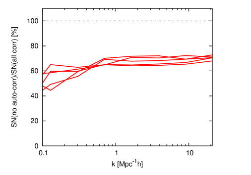
Figure 10: Relative change in the signal-to-noise in $f_{\delta,mn}$ if only shear tomography correlation functions $\xi_{\pm}^{(ij)}$ with $i\neq j$ (redshift slices with no overlap) are used for the estimation (minimum variance). The plot is based on a fiducial survey with $\sigma_{z}=0$. Different lines correspond to different $z$-bins. In total, roughly 30 percent of the signal-to-noise is lost.

Although the II- and GI-contaminations are an obvious concern for this kind of analysis, the focus of this paper is the performance of the new estimators under ideal conditions. We therefore defer a quantitative discussion of those effects to a future paper with the comment that the contamination can be partly removed by considering only slice pairs with little or no overlap in the tomography analysis in $\xi_{\pm}^{(ij)}$. To achieve this, we redid the aforementioned analysis for a fiducial survey with no redshift errors ($\sigma_{z}=0$), i.e., and exactly no overlap for $i\neq j$, and compared the relative change in signal-to-noise of an analysis that uses all tomography correlation functions to the signal-to-noise in a analysis that utilises only the $i\neq j$ correlators. The impact of omitting that piece of information on the significance of $\hat{\@vec{f}}_{\delta}$ is presented by Fig. 10: The significance drops by approximately 30 percent at all redshifts. The contaminations can possibly be more effectively removed by means of nulling techniques (Joachimi & Schneider, 2008). Since this is very likely to further degrade constraints on the 3D power spectra, we can speculate with the predictions above that significantly more survey area than $200\,\rm deg^{2}$ will then be needed for a proper reconstruction of $P_{\delta}(k,\chi)$.

4.7 B-mode matter band power spectrum

Finally, the estimator for the 3D matter band power spectrum, based on Eq. (2.1), presumes the absence of B-modes in the shear field, i.e., that shear-shear correlations vanish after a rotation of the source ellipticities $\epsilon$ by $\phi_{45}:=\pi/4$, hence after the transformation $\epsilon\mapsto{\rm e}^{-2{\rm i}\phi_{45}}\epsilon$. The presence of a B-mode component in $\xi_{\pm}^{(ij)}$ can potentially distort $\@vec{f}_{\delta}$. Whether such a contamination is present can be verified in an analysis by estimating $\@vec{f}^{\rm B}_{\delta}$ with all source ellipticities rotated in the data by $\phi_{45}$ (B-mode band power spectrum) and by estimating $\@vec{f}^{\rm EB}_{\delta}$ with only one source ellipticity in the two-point correlator $\xi_{\pm}^{(ij)}$ rotated by $\phi_{45}$ (E/B-mode cross-power spectrum). Hence, the inferred B-mode band powers $\@vec{f}^{\rm B}_{\delta}$ and $\@vec{f}^{\rm EB}_{\delta}$ that are inconsistent with zero indicate the presence and magnitude of such a contamination. We note that this only reveals possible B-mode issues in the data, but is by no means a sufficient and necessary condition for systematics in the data, since systematics could in principle only be present in the E-mode.

To obtain an estimator for $P_{\delta}(k,\chi)$ that is purely rooted in the E-mode components of the shear tomography correlations, it is also conceivable to devise the COSEBI formalism, which was proposed by Schneider et al. (2010). In this alternative framework, only the E-mode components of the two-point shear correlation functions are extracted. As the COSEBI values ${\rm E}_{n}$ are linear transformations of $\xi_{\pm}(\theta)$ on a finite interval $\vartheta_{0}\leq\theta\leq\vartheta_{1}$, they (a) can also be easily measured from the data and (b) must also be linear transformations of $\@vec{f}_{\delta}$

$$\@vec{E}={\@tens{V}}\@vec{f}_{\delta}\;,$$ (51)

where the COSEBI statistics ${\rm E}^{(ij)}_{n}$ up to order $n=1\ldots N_{\rm order}$ and pairs of redshift slices are assembled within the new data vector $\@vec{E}$. Therefore, one could use ${\@tens{V}}$ instead of ${\@tens{X}}$ and $\@vec{E}$ instead of $\@vec{\xi}$ in the previous estimator in Eq. (20) and the likelihood in Eq. (46) to implement a matter band-power spectrum reconstruction based on COSEBIs. Moreover, as shown by Asgari et al. (2012) and Eifler (2011), to estimate cosmological parameters with cosmic shear only a few COSEBIs modes are required. If this also turns out to be the case for the measurement of the band powers, this will dramatically reduce the size of the noise covariances involved, possibly simplifying their calculation or estimation from the data. It is unclear at this point, however, up to which order $N_{\rm order}$ COSEBIs are required to comprise essentially all information on $P_{\delta}(k,\chi)$.

Appendix A Numerical evaluation of basis functions

To calculate the contribution of a power band to a two-point correlator $\lambda_{mn}(\theta)$ on the sky, we note that all three families of basis functions in Eqs. (2.1), (2.2) and (2.3) can be written in the form

$$\theta^{2}\lambda_{mn}(\theta)=\int_{\chi_{n}}^{\chi_{n+1}}{\rm d}\chi\,g(\chi)\int\limits_{k_{m}f_{\rm k}(\chi)\theta}^{k_{m+1}f_{\rm k}(\chi)\theta}{\rm d}s\,s\,J_{n}(s)\,P^{\rm fid}\left(\frac{s}{f_{\rm k}(\chi)\theta},\chi\right)\;.$$ (52)

For a numerical evaluation of integrals of this type, we suggest approximating the inner $s$-integral with the sum

$$\Lambda_{mn}(\theta,\chi) := \int\limits_{k_{m}f_{\rm k}(\chi)\theta}^{k_{m+1}f_{\rm k}(\chi)\theta}{\rm d}s\,s\,J_{n}(s)\,P^{\rm fid}\left(\frac{s}{f_{\rm k}(\chi)\theta},\chi\right)$$

$$\approx \sum_{j=0}^{N_{\rm int}-1}P^{\rm fid}(\bar{k}_{j},\chi)\int\limits_{k_{j}f_{\rm k}(\chi)\theta}^{k_{j+1}f_{\rm k}(\chi)\theta}{\rm d}s\,s\,J_{n}(s)$$

$$= \sum_{j=0}^{N_{\rm int}-1}P^{\rm fid}(\bar{k}_{j},\chi)\left[{\cal J}_{n}(\hat{k}_{j+1}f_{\rm k}(\chi)\theta)-{\cal J}_{n}(\hat{k}_{j}f_{\rm k}(\chi)\theta)\right]\;,$$

where

$${\cal J}_{n}(x):=\left\{\begin{array}[]{ll}xJ_{1}(x)&,{\rm for}\leavevmode\nobreak\ n=0\\ 2-2J_{0}(x)-xJ_{1}(x)&,{\rm for}\leavevmode\nobreak\ n=2\\ 4+\left(x-\frac{8}{x}\right)J_{1}(x)-8J_{2}(x)&,{\rm for}\leavevmode\nobreak\ n=4\end{array}\right.$$ (54)

and $\bar{k}_{j}:=(\hat{k}_{j}+\hat{k}_{j+1})/2$, $\hat{k}_{j}:=k_{m}+j\Delta k$ and $\Delta k:=(k_{m+1}-k_{m})/N_{\rm int}$ for $N_{\rm int}\sim 100$ integration intervals. Where $P^{\rm fid}(k,\chi)=1$ is a reference power spectrum, the foregoing sum is exact for $N_{\rm int}=1$. The outer $\chi$-integral

$$\theta^{2}\lambda_{mn}(\theta)=\int_{\chi_{n}}^{\chi_{n+1}}{\rm d}\chi\,g(\chi)\Lambda_{mn}(\theta,\chi)$$ (55)

can be computed with Romberg’s method (Press et al., 1992).

Appendix B Generation of mock catalogues

Here we outline an algorithm for making Monte Carlo realisations of shear tomography data, including galaxy clustering and galaxy-galaxy lensing.

The convergence fields are simulated as Gaussian random fields, whereas galaxy clustering obeys log-normal statistics (Coles & Jones, 1991). Log-normal statistics, or statistics with a lower bound $\kappa_{\rm g}\geq-1$ for the number density contrast $\kappa_{\rm g}$, is essential for a catalogue of mock galaxy positions. For the simulation, we use $2048\times 2048\,\rm pixel^{2}$ grids, spanning an angular area of $4\times 4\,\rm deg^{2}$, out of which just $2\times 2\,\rm deg^{2}$ subfields are taken after performing our realisation. The simulation comprises $N_{z}=5$ redshift slices. The Monte Carlo recipe is similar to the approach outlined in Coles (1988), Coles (1989), and Coles & Jones (1991), but generalised to the simultaneous realisation of a set of random fields, both Gaussian and log-normal, with defined cross-correlations. As a model of the 3D dark matter power spectrum, the prescription of Smith et al. (2003) is employed.

For the generation of correlated random fields, we follow the approach of Simon et al. (2004), but now also include the clustering of galaxies as additional degree of freedom. A realisation is performed on grids of angular size $A$, namely one lensing convergence grid $\kappa^{(i)}(\@vec{\theta})$ and one galaxy number density $\kappa_{\rm g}^{(i)}(\@vec{\theta})$ grid for each of the $i=1\ldots N_{z}$ galaxy subsamples. The Fourier modes for identical $\@vec{\ell}$ vectors of all $2N_{z}$ grids are compiled as one vector

$$\tilde{\@vec{v}}(\@vec{\ell})=\left(\tilde{\kappa}^{(1)}(\@vec{\ell}),\tilde{\kappa}^{(2)}(\@vec{\ell}),\ldots,\tilde{\kappa}_{\rm g}^{(1)}(\@vec{\ell}),\tilde{\kappa}_{\rm g}^{(2)}(\@vec{\ell}),\ldots\right)^{\rm t}$$ (56)

and are randomly generated independently from all other modes by (Sect. IV.B. in Hu & Keeton, 2002)

$$\tilde{\@vec{v}}(\@vec{\ell})=\frac{1}{\sqrt{2A}}{\@tens{L}}_{S}\left(\@vec{g}+{\rm i}\@vec{g}^{\prime}\right)\;,$$ (57)

where $g_{i},g^{\prime}_{i}\curvearrowleft{\cal N}(0,1)$ are vectors of normally distributed random numbers, with mean zero and unity variance, having the same number of elements as $\@vec{\tilde{v}}(\@vec{\ell})$. The matrix ${\@tens{L}}_{S}$ denotes the Cholesky decomposition, ${\@tens{S}}={\@tens{L}}_{S}{\@tens{L}}_{S}^{\rm t}$, of the Fourier mode covariance matrix

$${\@tens{S}}=\left(\begin{array}[]{ll}{\@tens{P}}_{\kappa}(\ell)&{\@tens{P}}_{\kappa\rm g}(\ell)\\ {\@tens{P}}_{\kappa\rm g}(\ell)&{\@tens{P}}_{\rm g}(\ell)\end{array}\right)\;.$$ (58)

This matrix ${\@tens{S}}$ consists of three sub-matrices, describing (a) the auto- and cross-correlations between the convergence fields by

$$[{\@tens{P}}_{\kappa}(\ell)]_{ij}=\frac{9H_{0}^{4}\Omega_{\rm m}^{2}}{4c^{4}}\int_{0}^{\chi_{\rm h}}{\rm d}\chi\frac{\overline{W}^{(i)}(\chi)\overline{W}^{(j)}(\chi)}{a(\chi)^{2}}P_{\delta}\left(\frac{\ell}{f_{\rm k}(\chi)},\chi\right)\;,$$ (59)

(b) the lenses number density and convergence cross-correlations

$$[{\@tens{P}}_{\kappa\rm g}(\ell)]_{ij}=\frac{3H_{0}^{2}\Omega_{\rm m}}{2c^{2}}\int_{0}^{\chi_{\rm h}}{\rm d}\chi\frac{\overline{W}^{(i)}(\chi)q_{\chi}^{(j)}(\chi)}{f_{\rm k}(\chi)a(\chi)}P_{\delta\rm g}\left(\frac{\ell}{f_{\rm k}(\chi)},\chi\right)\;,$$ (60)

and (c) the auto- and cross-correlations between the lens number density fields

$$[{\@tens{P}}_{\rm g}(\ell)]_{ij}=\hat{P}^{(ij)}_{\rm g}(\ell)\;,$$ (61)

which needs further discussion below. For the scope of this paper, lenses are just random subsets of the source samples, i.e. $p_{\chi}^{(i)}(\chi)=q_{\chi}^{(i)}(\chi)$. Moreover, galaxies are assumed to be unbiased, i.e., $b(k,\chi)=r(k,\chi)=1$.

Case (c) in Eq. (58) requires a special treatment to ensure that a log-normal random field can be realised. We obtain $\hat{P}^{(ij)}_{\rm g}(\ell)$ from

$$P_{\rm g}^{(ij)}(\ell)=\int_{0}^{\chi_{\rm h}}{\rm d}\chi\frac{q_{\chi}^{(i)}(\chi)q_{\chi}^{(j)}(\chi)}{f_{\rm k}^{2}(\chi)}P_{\rm g}\left(\frac{\ell}{f_{\rm k}(\chi)},\chi\right)$$ (62)

in three steps:

$${\rm step\leavevmode\nobreak\ 1:} \omega^{(ij)}(\theta)=\frac{1}{2\pi}\int_{0}^{\infty}{\rm d}\ell\,\ell\,J_{0}(\ell\theta)P_{\rm g}^{(ij)}(\ell)\;,$$ (63)

$${\rm step\leavevmode\nobreak\ 2:} \hat{\omega}^{(ij)}(\theta)=\ln{(\omega^{(ij)}(\theta)+1)}\;,$$ (64)

$${\rm step\leavevmode\nobreak\ 3:} \hat{P}_{\rm g}^{(ij)}(\ell)=2\pi\int_{0}^{\infty}{\rm d}\theta\,\theta\,J_{0}(\ell\theta)\hat{\omega}^{(ij)}(\theta)\;.$$ (65)

This transformation rule is found because a log-normal random field with lower limit $\kappa_{\rm ln}\geq-1$ can be generated from a random Gaussian field $\kappa_{\rm g}$ via (Coles & Jones, 1991)

$$\kappa_{\rm ln}(\@vec{\theta})={\rm e}^{\kappa_{\rm g}(\@vec{\theta})-\sigma^{2}_{\rm g}/2}-1\;,$$ (66)

if the two-point correlation function of the underlying Gaussian process is

$$\omega_{\rm g}(\theta)=\Big{\langle}\kappa_{\rm g}(\theta^{\prime})\kappa_{\rm g}(\theta^{\prime}+\theta)\Big{\rangle}=\ln{\bigl{(}1+\omega_{\rm ln}(\theta)\bigr{)}}$$ (67)

compared to the two-point correlations $\omega_{\rm ln}(\theta)$ in the log-normal random field, where $\sigma_{\rm g}^{2}$ is the variance in $\kappa_{\rm g}$. By the same argument, however, the cross-power between galaxy number density and convergence grid in ${\@tens{P}}_{\kappa\rm g}(\ell)$ remains unchanged because

$$\Big{\langle}\kappa_{\rm ln}(\theta^{\prime})\kappa_{\rm g}(\theta^{\prime}+\theta)\Big{\rangle}=$$

$$\Big{\langle}\left({\rm e}^{\kappa_{\rm g}(\theta^{\prime})-\sigma_{\rm g}^{2}/2}-1\right)\kappa_{\rm g}(\theta^{\prime}+\theta)\Big{\rangle}=\Big{\langle}\kappa_{\rm g}(\theta^{\prime})\kappa_{\rm g}(\theta^{\prime}+\theta)\Big{\rangle}\;,$$

for

$$\Big{\langle}f(\delta_{1},\delta_{2})\Big{\rangle} = \int{\rm d}\delta_{1}{\rm d}\delta_{2}P(\delta_{1},\delta_{2})f(\delta_{1},\delta_{2})\;,$$ (69)

$$P(\delta_{1},\delta_{2}) = \frac{1}{2\pi\sigma_{1}\sigma_{2}\sqrt{1-\psi(\theta)^{2}}}\,\times$$

$$\exp{\left(-\frac{\delta_{1}^{2}\sigma_{2}^{2}+\delta_{2}^{2}\sigma_{1}^{2}-2\omega(\theta)\delta_{1}\delta_{2}}{2\sigma_{1}^{2}\sigma_{2}^{2}(1-\psi(\theta)^{2})}\right)}\;,$$

where $\sigma_{1}^{2}=\Big{\langle}\delta_{1}^{2}\Big{\rangle}$, $\sigma_{2}^{2}=\Big{\langle}\delta_{2}^{2}\Big{\rangle}$ and $\psi(\theta)=\omega(\theta)/(\sigma_{1}\sigma_{2})$, and $P(\delta_{1},\delta_{2})$ is a bivariate Gaussian p.d.f.

After all $\ell$-modes $\@vec{\tilde{v}}(\@vec{\ell})$ have been realised, the grids are Fourier transformed to real space to yield the convergence fields and the galaxy number density contrast fields on a grid. The galaxy number density contrasts represent only the underlying Gaussian fields, $\kappa_{\rm g}$, so far and hence still need to be transformed into the log-normal density contrasts. This is done by applying the additional mapping $\kappa_{\rm ln}={\rm e}^{\kappa_{\rm g}-\sigma^{2}_{\rm g}/2}-1$ for every pixel. We acquire $\sigma_{\rm g}^{2}$ from the given realisation of the Gaussian random field.

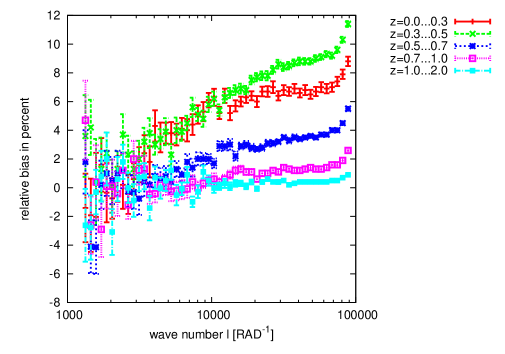
Figure 11: Relative bias $\Delta P_{\rm m}/P_{\rm m}^{\rm fid}$ (percent) in the power spectrum of the log-normal random field realisation for different redshift bins as function of angular mode wave number $\ell$.

The mapping, however, is only an approximation because $\kappa_{\rm g}$ is actually a realisation of a smoothed Gaussian field, which is denoted here by an overline:

$$\overline{\kappa}_{\rm g}(\@vec{\theta}) = \int{\rm d}^{2}\theta^{\prime}\,\kappa_{\rm g}(\@vec{\theta}^{\prime})W(\@vec{\theta}-\@vec{\theta}^{\prime})\;.$$ (71)

The function $W(\@vec{\theta})$ represents the pixel smoothing function, which is assumed to be normalised to unity by definition, i.e. $\int{\rm d}^{2}\theta W(\@vec{\theta})=1$. Applying the exponential mapping to $\overline{\kappa}_{\rm g}$ thus assumes that a similar relation between smoothed underlying Gaussian and smoothed log-normal field $\overline{\kappa}_{\rm ln}$ approximately holds, namely

$$\overline{\kappa}_{\rm ln}(\@vec{\theta})\approx{\rm e}^{\overline{\kappa}_{\rm g}(\@vec{\theta})-\sigma^{2}_{\rm g}/2}-1\;.$$ (72)

The relation between the smoothed fields would be exact, if the mapping were linear. The approximation has higher accuracy for less fluctuating $\overline{\kappa}_{\rm g}$ and vice versa. For this paper, we employ mock data in which galaxies perfectly trace the dark matter distribution at all redshifts. As dark matter fluctuations decline towards higher redshift, the above approximation provides a gain in accuracy for higher redshift bins. With the outlined method, we achieve an accuracy in the log-normal field power of better than $10\%$ and on $\ell$-average several percent for the fiducial survey employed (Fig. 11). We consider this to be sufficient for our purposes, although a better treatment of this bias may be desirable for future applications.

Finally, the grids $\kappa^{(i)}_{\rm g}$ and $\kappa^{(i)}$ serve as a basis for the $i$th redshift slice of the mock survey: a candidate galaxy position $\@vec{\theta}$ is drawn randomly as the position on the grid from a uniform PDF. The position is accepted, if $x\leq 1+\kappa^{(i)}_{\rm g}(\@vec{\theta})$ where $x\in[0,1]$ is also a random number from a uniform PDF, in accordance with Coles & Jones (1991) for grids large enough to accommodate mostly no more than one galaxy per pixel. This algorithm thus utilises a Poisson process to sample the galaxy number density contrast $\kappa^{(i)}_{\rm g}$ with a discrete set of galaxy positions. As a complex source ellipticity, we adopt $\gamma^{(i)}(\@vec{\theta})+\epsilon_{\rm s}$, where $\gamma^{(i)}$ is the shear field corresponding to $\kappa^{(i)}$ (Kaiser & Squires, 1993) and $\epsilon_{\rm s}$ the random intrinsic shape of the galaxy drawn from a statistically independent PDF. This process is repeated until the desired number density of galaxies for the $i$th redshift bin is reached.

References

- Asgari et al. (2012) Asgari, M., Schneider, P., & Simon, P. 2012, arXiv:1201.2669
- Bacon et al. (2005) Bacon, D. J., Taylor, A. N., Brown, M. L., & et al. 2005, MNRAS, 363, 723
- Bartelmann & Schneider (2001) Bartelmann, M. & Schneider, P. 2001, Phys. Rep, 340, 291
- Baugh & Efstathiou (1994) Baugh, C. M. & Efstathiou, G. 1994, MNRAS, 267, 323
- Blandford et al. (1991) Blandford, R. D., Saust, A. B., Brainerd, T. G., & Villumsen, J. V. 1991, MNRAS, 251, 600
- Bouchet et al. (1993) Bouchet, F. R., Strauss, M. A., Davis, M., et al. 1993, ApJ, 417, 36
- Castro et al. (2005) Castro, P. G., Heavens, A. F., & Kitching, T. D. 2005, Phys. Rev. D, 72, 023516
- Clifton et al. (2011) Clifton, T., Ferreira, P. G., Padilla, A., & Skordis, C. 2011, arXiv:1106.2476
- Clowe et al. (2006) Clowe, D., Bradač, M., Gonzalez, A. H., & et al. 2006, ApJ(Lett), 648, L109
- Coles (1988) Coles, P. 1988, MNRAS, 234, 509
- Coles (1989) Coles, P. 1989, MNRAS, 238, 319
- Coles & Jones (1991) Coles, P. & Jones, B. 1991, MNRAS, 248, 1
- Dodelson (2003) Dodelson, S. 2003, Modern cosmology, ed. Dodelson, S.
- Eifler (2011) Eifler, T. 2011, MNRAS, 418, 536
- Guzik & Seljak (2001) Guzik, J. & Seljak, U. 2001, MNRAS, 321, 439
- Hartlap et al. (2009) Hartlap, J., Schrabback, T., Simon, P., & Schneider, P. 2009, A&A, 504, 689
- Hartlap et al. (2007) Hartlap, J., Simon, P., & Schneider, P. 2007, A&A, 464, 399
- Heitmann et al. (2010) Heitmann, K., White, M., Wagner, C., Habib, S., & Higdon, D. 2010, ApJ, 715, 104
- Heymans et al. (2006) Heymans, C., White, M., Heavens, A., Vale, C., & van Waerbeke, L. 2006, MNRAS, 371, 750
- Hilbert et al. (2011) Hilbert, S., Hartlap, J., & Schneider, P. 2011, A&A, 536, A85
- Hilbert et al. (2009) Hilbert, S., Hartlap, J., White, S. D. M., & Schneider, P. 2009, A&A, 499, 31
- Hildebrandt et al. (2008) Hildebrandt, H., Wolf, C., & Benítez, N. 2008, A&A, 480, 703
- Hirata & Seljak (2004) Hirata, C. M. & Seljak, U. 2004, Phys. Rev. D, 70, 063526
- Hoekstra et al. (2002) Hoekstra, H., van Waerbeke, L., Gladders, M. D., Mellier, Y., & Yee, H. K. C. 2002, ApJ, 577, 604
- Hu (2002) Hu, W. 2002, Phys. Rev. D, 66, 083515
- Hu & Keeton (2002) Hu, W. & Keeton, C. R. 2002, Phys. Rev. D, 66, 063506
- Hu & White (2001) Hu, W. & White, M. 2001, ApJ, 554, 67
- Jing et al. (2006) Jing, Y. P., Zhang, P., Lin, W. P., Gao, L., & Springel, V. 2006, ApJ, 640, L119
- Joachimi & Schneider (2008) Joachimi, B. & Schneider, P. 2008, A&A, 488, 829
- Kaiser (1992) Kaiser, N. 1992, ApJ, 388, 272
- Kaiser & Squires (1993) Kaiser, N. & Squires, G. 1993, ApJ, 404, 441
- Keitel & Schneider (2011) Keitel, D. & Schneider, P. 2011, A&A, 534, A76
- Kiessling et al. (2011) Kiessling, A., Heavens, A. F., Taylor, A. N., & Joachimi, B. 2011, MNRAS, 414, 2235
- Kitching et al. (2011) Kitching, T. D., Heavens, A. F., & Miller, L. 2011, MNRAS, 413, 2923
- Komatsu et al. (2011) Komatsu, E., Smith, K. M., & Dunkley, e. a. 2011, ApJS, 192, 18
- Landy & Szalay (1993) Landy, S. D. & Szalay, A. S. 1993, ApJ, 412, 64
- Laureijs et al. (2011) Laureijs, R., Amiaux, J., Arduini, S., et al. 2011, arXiv:1110.3193
- Leonard et al. (2012) Leonard, A., Dupé, F.-X., & Starck, J.-L. 2012, A&A, 539, A85
- Li et al. (2011) Li, B., King, L. J., Zhao, G.-B., & Zhao, H. 2011, MNRAS, 415, 881
- MacKay (2003) MacKay, J. D. 2003, Information Theory, Inference, and Learning Algorithms (Cambridge University Press, Cambridge, UK)
- Martínez & Saar (2002) Martínez, V. J. & Saar, E. 2002, Statistics of the Galaxy Distribution, ed. Martínez, V. J. & Saar, E. (Chapman and Hall/CRC)
- Massey et al. (2007a) Massey, R., Rhodes, J., & Ellis, R. 2007a, Nat, 445, 286
- Massey et al. (2007b) Massey, R., Rhodes, J., Leauthaud, A., et al. 2007b, ApJS, 172, 239
- Miralda-Escude (1991) Miralda-Escude, J. 1991, ApJ, 380, 1
- Mo et al. (2010) Mo, H., van den Bosch, F. C., & White, S. 2010, Galaxy Formation and Evolution, ed. Mo, H., van den Bosch, F. C., & White, S.
- Narayan (1989) Narayan, R. 1989, ApJ, 339, L53
- Peacock (1999) Peacock, J. A. 1999, Cosmological Physics, ed. Cambridge, UK: Cambridge University Press, ISBN 052141072X
- Peacock & Dodds (1996) Peacock, J. A. & Dodds, S. J. 1996, MNRAS, 280, L19
- Peebles (1980) Peebles, P. J. E. 1980, The large-scale structure of the universe (Princeton University Press, USA)
- Pen et al. (2003) Pen, U.-L., Lu, T., van Waerbeke, L., & Mellier, Y. 2003, MNRAS, 346, 994
- Pen et al. (2002) Pen, U.-L., Van Waerbeke, L., & Mellier, Y. 2002, ApJ, 567, 31
- Press et al. (1992) Press, W. H., Teukolsky, S. A., Vetterling, W. T., & Flannery, B. P. 1992, Numerical recipes in C. The art of scientific computing (Cambridge: University Press, —c1992, 2nd ed.)
- Schneider (1998) Schneider, P. 1998, ApJ, 498, 43
- Schneider (2006) Schneider, P. 2006, in Saas-Fee Advanced Course 33: Gravitational Lensing: Strong, Weak and Micro, ed. G. Meylan, P. Jetzer, P. North, P. Schneider, C. S. Kochanek, & J. Wambsganss, 269–451
- Schneider et al. (2010) Schneider, P., Eifler, T., & Krause, E. 2010, A&A, 520, 116
- Schneider & Hartlap (2009) Schneider, P. & Hartlap, J. 2009, A&A, 504, 705
- Schneider et al. (1998) Schneider, P., van Waerbeke, L., Jain, B., & Kruse, G. 1998, MNRAS, 296, 873
- Schneider et al. (2002) Schneider, P., van Waerbeke, L., Kilbinger, M., & Mellier, Y. 2002, A&A, 396, 1
- Schrabback et al. (2010) Schrabback, T., Hartlap, J., & Joachimi, B. 2010, A&A, 516, 63
- Seljak et al. (2005) Seljak, U., Makarov, A., Mandelbaum, R., et al. 2005, Phys. Rev. D, 71, 043511
- Semboloni et al. (2011) Semboloni, E., Hoekstra, H., Schaye, J., van Daalen, M. P., & McCarthy, I. G. 2011, arXiv:1105.1075
- Semboloni et al. (2007) Semboloni, E., van Waerbeke, L., Heymans, C., et al. 2007, MNRAS, 375, L6
- Simon et al. (2007) Simon, P., Hetterscheidt, M., Schirmer, M., et al. 2007, A&A, 461, 861
- Simon et al. (2012) Simon, P., Heymans, C., Schrabback, T., et al. 2012, MNRAS, 419, 998
- Simon et al. (2004) Simon, P., King, L. J., & Schneider, P. 2004, A&A, 417, 873
- Smith et al. (2003) Smith, R. E., Peacock, J. A., Jenkins, A., et al. 2003, MNRAS, 341, 1311
- Somogyi & Smith (2010) Somogyi, G. & Smith, R. E. 2010, Phys. Rev. D, 81, 023524
- Springel et al. (2005) Springel, V., White, S. D. M., & Jenkins, A. e. a. 2005, Nature, 435, 629
- Tegmark et al. (2004) Tegmark, M., Blanton, M. R., Strauss, M. A., & etl a. 2004, ApJ, 606, 702
- Tegmark & Peebles (1998) Tegmark, M. & Peebles, P. J. E. 1998, ApJ, 500, 79
- Tegmark et al. (1997) Tegmark, M., Taylor, A. N., & Heavens, A. F. 1997, ApJ, 480, 22
- Tereno et al. (2009) Tereno, I., Schimd, C., Uzan, J.-P., et al. 2009, A&A, 500, 657
- Uzan & Bernardeau (2001) Uzan, J.-P. & Bernardeau, F. 2001, Phys. Rev. D, 64, 083004
- van Daalen et al. (2011) van Daalen, M. P., Schaye, J., Booth, C. M., & Dalla Vecchia, C. 2011, MNRAS, 415, 3649
- van Waerbeke (1998) van Waerbeke, L. 1998, A&A, 334, 1
- van Waerbeke (2010) van Waerbeke, L. 2010, MNRAS, 401, 2093
- Van Waerbeke & Mellier (2003) Van Waerbeke, L. & Mellier, Y. 2003, arXiv:astro-ph/0305089
- VanderPlas et al. (2011) VanderPlas, J. T., Connolly, A. J., Jain, B., & Jarvis, M. 2011, ApJ, 727, 118
- Weinberg et al. (2004) Weinberg, D. H., Davé, R., Katz, N., & Hernquist, L. 2004, ApJ, 601, 1
- White & Hu (2000) White, M. & Hu, W. 2000, ApJ, 537, 1
- Yoshikawa et al. (2001) Yoshikawa, K., Taruya, A., Jing, Y. P., & Suto, Y. 2001, ApJ, 558, 520
- Zaroubi et al. (1995) Zaroubi, S., Hoffman, Y., Fisher, K. B., & Lahav, O. 1995, ApJ, 449, 446
- Zehavi et al. (2011) Zehavi, I., Zheng, Z., Weinberg, D. H., & et al. 2011, ApJ, 736, 59
- Zhan & Knox (2004) Zhan, H. & Knox, L. 2004, ApJ, 616, L75