Electron spin orientation under in-plane optical excitation in GaAs quantum wells

Abstract

We study the optical orientation of electron spins in GaAs/AlGaAs quantum wells for excitation in the growth direction and for in-plane excitation. Time- and polarization-resolved photoluminescence excitation measurements show, for resonant excitation of the heavy-hole conduction band transition, a negligible degree of electron spin polarization for in-plane excitation and nearly 100% for excitation in the growth direction. For resonant excitation of the light-hole conduction band transition, the excited electron spin polarization has the same (opposite) direction for in-plane excitation (in the growth direction) as for excitation into the continuum. The experimental results are well explained by an accurate multiband theory of excitonic absorption taking fully into account electron-hole Coulomb correlations and heavy-hole light-hole coupling.

I Introduction

The efficient injection and detection of spin-polarized carriers in semiconductor quantum wells (QWs) is a field of intensive research. zut04 Among various approaches that have been used to achieve this goal, optical selection rules dya84 have often played an important role. In many cases, spin-polarized electrons are both optically excited and optically detected. hae98 ; cro05 ; gil09 Other approaches combine optical excitation of spin-polarized carriers with electrical detection schemes utilizing, e.g., orientation- and spin-dependent charge currents. gan03a Still others employ electrical injection of spin-polarized carriers, e.g., via paramagnetic semiconductors as spin aligners, and probe optically by polarization-resolved photoluminescence (PL) spectroscopy. oes99 ; fie99 ; jon00 All these experiments demonstrate that optical selection rules are a very useful tool to study semiconductor spintronics since they directly relate the light polarization with the spin polarization of the electrons. dya84 In principle, the optical selection rules also determine the hole spin polarization in the valence band, yet this polarization usually decays so rapidly dam91 ; hil02 that it can be neglected in most experiments. Nonetheless, recent experiments have also exploited the optical orientation for hole systems. kor10 ; pri10a

The optical selection rules in QWs have been investigated in detail for optical excitation by circularly polarized light in the growth direction, pfa05 but the selection rules for spin excitation in the plane of the QW have not been studied systematically so far, to the best of our knowledge. Such an in-plane excitation or detection of electron spin polarization plays an important role in a variety of experiments. For example, Ohno et al. measured the degree of circular polarization of the side-emitted electroluminescence due to the heavy-hole (HH) transition of electrically injected carriers. ohn99a ; oes99a Oestreich et al. studied spin precession in a magnetic field after in-plane excitation of the light-hole (LH) transition to directly measure the sign of the effective $g$ factor of electrons in a QW. oes98

In this article, we present a detailed study of the optical orientation of electron spins in a GaAs multi-QW using a light beam propagating parallel to the plane of the two-dimensional (2D) system. A circularly polarized laser pulse is focused on the cleaved edge of the QWs, creating spin-polarized electrons in the wells. Application of an in-plane magnetic field perpendicular to the excitation direction leads to spin precession, which we observe in the optical emission in the growth direction of the 2D system. From the time- and polarization-resolved PL, we obtain the initial degree of electron spin polarization $P_{0}$ which is studied as a function of the excitation energy. We compare our measured results with an accurate theory of excitonic absorption taking fully into account electron-hole Coulomb correlations and HH-LH coupling.

We begin in Sec. II by discussing a simplified, qualitative model that incorporates the main features of optical orientation for arbitrary excitation and polarization directions. The experimental setup and methods for data analysis are described in Sec. III. Section IV.1 presents as a reference frame the results for excitation in the growth direction, while the rest of Sec. IV is devoted to in-plane excitation. The accurate theoretical model is presented in Sec. V. We end with conclusions in Sec. VI.

II Qualitative Model for Optical Orientation

For QWs made of direct semiconductors such as GaAs, the main features of optical orientation can be understood in a simplified version of the full theory developed in Sec. V. In this simplified model, we neglect the in-plane dispersion of the electron and hole states (i.e., in-plane wave vector ${\bm{\mathrm{k}}}=0$) as well as the ${\bm{\mathrm{k}}}\cdot{\bm{\mathrm{p}}}$ coupling between conduction and valence band states so that the subband states are represented by their dominant spinor components. If the exciting light is characterized by a polarization vector $\hat{{\bm{\mathrm{e}}}}=(e_{x},e_{y},e_{z})$, the optically excited electrons are characterized by the $2\times 2$ spin density matrix scalar

$$\dot{\varrho}(\omega)\equiv\frac{d}{dt}\,\rho(\omega)=\mathcal{C}\sum_{\alpha}\left(\varrho_{0}^{\alpha}\openone_{2\times 2}+{\bm{\mathrm{s}}}^{\alpha}\cdot{\bm{\mathrm{\sigma}}}\right)\delta(\hbar\omega-E_{\alpha}),$$ (1)

where the sum runs over HH and LH states, and ${\bm{\mathrm{\sigma}}}$ is the vector of Pauli matrices. We have, for the HH transitions,

$$\varrho_{0}^{\mathrm{HH}} = |e_{x}|^{2}+|e_{y}|^{2}$$ (2a)

$$s_{x}^{\mathrm{HH}} = s_{y}^{\mathrm{HH}}=0$$ (2b)

$$s_{z}^{\mathrm{HH}} = 2\,\Im\left(e_{x}e_{y}^{\ast}\right)$$ (2c)

and for the LH transitions

$$\varrho_{0}^{\mathrm{LH}} = {\textstyle\frac{1}{3}}|e_{x}|^{2}+{\textstyle\frac{1}{3}}|e_{y}|^{2}+{\textstyle\frac{4}{3}}|e_{z}|^{2}$$ (3a)

$$s_{x} = {\textstyle\frac{4}{3}}\,\Im\left(e_{y}e_{z}^{\ast}\right)$$ (3b)

$$s_{y} = {\textstyle\frac{4}{3}}\,\Im\left(e_{z}e_{x}^{\ast}\right)$$ (3c)

$$s_{z} = -{\textstyle\frac{2}{3}}\,\Im\left(e_{x}e_{y}^{\ast}\right),\hskip 20.00003pt$$ (3d)

which reflects the well-known Clebsch-Gordan coefficients characterizing the dipole matrix elements between spin-$1/2$ states in the conduction band and (effective) spin-$3/2$ states in the valence band. dya84 Finally, we have

$$\mathcal{C}=\frac{e^{2}A^{2}_{0}}{2m_{0}}\frac{P^{2}}{\hbar\omega},$$ (4)

where $A_{0}$ denotes the amplitude of the vector potential of the light field and $P$ is Kane’s momentum matrix element. win03 The quantity $\mathcal{C}$ is essentially a constant for optical transitions close to the fundamental absorption edge. We see that, apart from the prefactor $\mathcal{C}$ the spin density matrix depends only on the components of the polarization vector $\hat{{\bm{\mathrm{e}}}}$ and the excitation energies $E_{\mathrm{HH}}$ and $E_{\mathrm{LH}}$ for HH and LH transitions. (We have ignored the trivial selection rule that we get a large oscillator strength for optical transitions only if the envelope functions for the electron and hole state have the same number of nodes.) Similar results for bulk material were previously obtained by Dymnikov et al.dym76

Apart from a constant prefactor [see Eq. (20) below], the absorption coefficient is then given by

$$\alpha(\omega)\propto\operatorname{tr}\dot{\varrho}=2\mathcal{C}\sum_{\alpha}\varrho_{0}^{\alpha}\,\delta(\hbar\omega-E_{\alpha}),$$ (5a)

where $$\operatorname{tr}$$ denotes the trace, and the spin polarization induced by a steady-state optical excitation becomes

$${\bm{\mathrm{P}}}(\omega)=\frac{\operatorname{tr}{\bm{\mathrm{\sigma}}}\dot{\varrho}}{\operatorname{tr}\dot{\varrho}}=\left\{\begin{array}[]{cs{2em}l}{\bm{\mathrm{s}}}^{\mathrm{HH}}/\varrho_{0}^{\mathrm{HH}},\hfil\hskip 20.00003pt&\hbar\omega=E_{\mathrm{HH}}\\[4.30554pt] {\bm{\mathrm{s}}}^{\mathrm{LH}}/\varrho_{0}^{\mathrm{LH}},\hfil\hskip 20.00003pt&\hbar\omega=E_{\mathrm{LH}}.\end{array}\right.$$ (5b)

Equations (5) can be easily evaluated for different polarization vectors $\hat{{\bm{\mathrm{e}}}}$. They include the well-known result dya84 ; pfa05 that, for excitation in the growth direction, the HH transitions are three times more efficient than the LH transitions (independendent of the polarization $\hat{{\bm{\mathrm{e}}}}$). With circularly polarized light [$\hat{{\bm{\mathrm{e}}}}={\textstyle\frac{1}{\sqrt{2}}}(1,\pm i,0)$] we obtain for both HH and LH transitions a complete electron spin polarization ($|{\bm{\mathrm{P}}}|=1$) in the $z$ direction that is opposite in sign for HH and LH transitions. It also follows from these equations that an in-plane excitation can give rise to both HH and LH transitions. Yet the details depend on the polarization $\hat{{\bm{\mathrm{e}}}}$. HH states do not couple to $e_{z}$ from which it follows immediately that an electron spin polarization via in-plane excitation of HH transitions is not possible. fie03 ; oes05 Only LH transitions with circularly polarized light [e.g., $\hat{{\bm{\mathrm{e}}}}={\textstyle\frac{1}{\sqrt{2}}}(1,0,\pm i)$] can give rise to a spin polarization of the electron states with a maximum $|{\bm{\mathrm{P}}}|=4/5$.

While Eqs. (1) and (5) allow one to understand the main features of optical orientation in QWs, these results get modified by the details of band structure such as HH-LH coupling [Eq. (22) below] and the excitonic Coulomb coupling between the single-particle states [Eq. (25)].

III Experimental Methods

Our sample is a multi-QW structure consisting of $15$ layers of GaAs/Al_0.3Ga_0.7As QWs with a well width of $14$ nm separated by barriers with a thickness of $10$ nm. The structure is grown on a $(001)$-oriented GaAs substrate and sandwiched between layers of 500 nm and 490 nm Al_0.3Ga_0.7As. The sample is of a very high quality, which has been confirmed by absorption measurements [see, e.g., the left column in Fig. 3(c) and measurements on a very similar sample containing 10 instead of 15 QWs in Ref. loe02, ]. The Stokes shift is, at most, of the order of $0.3$ meV, which is the resolution limit of the experimental setup.

In the following, we present measurements of the initial degree of spin polarization for two geometries of optical excitation. First, we perform a control experiment, where the sample is excited with circularly polarized laser pulses in the growth direction. We label the growth direction of the sample the $z$ axis, while the $x$ and $y$ directions are oriented in the plane of the QW [see Fig. 1(c)]. The experimental setup for this measurement as well as the techniques for data analysis is described in detail in Ref. pfa05, . Second, we focus the circularly polarized laser pulses on the cleaved edge of the sample and excite electrons with a spin polarization in the plane of the QW ($y$ direction). The setup for the latter experiments is described in detail in the following.

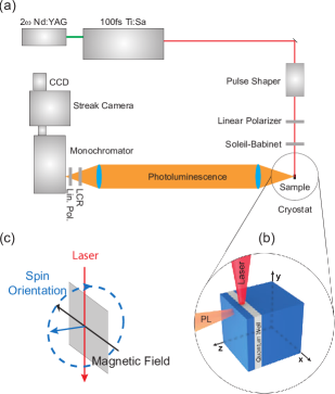
Figure 1: (Color online) (a) Experimental setup of the time-resolved PL measurements, (b) geometry for laser excitation as well as PL detection, and (c) sketch of the precession of the spin orientation (blue arrow) around the applied in-plane magnetic field (black arrow).

Figure 1(a) depicts the experimental setup for the time- and polarization-resolved PL measurements. The sample is mounted in Voigt configuration in a He gas flow cryostat in a superconducting magnet, cooled to a lattice temperature of 10 K, and excited by pulses from a femtosecond mode-locked Ti:sapphire laser with a repetition rate of $80$ MHz. A pulse shaper reduces the spectral linewidth of the $100$ fs laser pulses to $0.8$ nm full width at half-maximum (FWHM) and a Soleil-Babinet compensator adjusts the polarization of the laser pulses at the sample surface to circular polarization. Unless stated otherwise, the time-averaged excitation power is $1$ mW. The exciting laser light is propagating in the $y$ direction. An in-plane magnetic field $B_{x}$ gives rise to Larmor precession of the electron spins around $B_{x}$ [also called spin quantum beats (SQB), see Fig 1(c)] with the Larmor frequency $\omega_{L}=g^{\ast}\mu_{B}B_{x}/\hbar$, where $g^{\ast}$ is the effective electron $g$ factor, $\hbar$ is the Planck constant, and $\mu_{B}$ is the Bohr magneton. We detect the PL components along the $z$ axis, i.e., we detect the projection of the electron spin orientation on the $z$ axis which oscillates with the frequency $\omega_{L}$. For this purpose, the intensities of the left and right circularly polarized PL components $I_{\pm}(t)$ are measured separately using an electrically tunable liquid-crystal retarder (LCR), a linear polarizer, and a synchroscan streak camera providing temporal and spectral resolutions of $15$ ps and $7$ meV, respectively. The resulting time-dependent degree of optical polarization is defined as

$$P_{\mathrm{opt}}^{z}(t)=\frac{I_{+}(t)-I_{-}(t)}{I_{+}(t)+I_{-}(t)}.$$ (6)

At $t=0$, the electron spins are initially oriented along the $y$ axis so that the measured $P_{\mathrm{opt}}^{z}(t=0)$ is zero. After $1/4$ of the oscillation period, $P_{\mathrm{opt}}^{z}$ has either a maximum or a minimum, depending on the magnetic field direction and the sign of $g^{\ast}$. oes98 In order to determine the initial electron spin polarization $P_{0}$ at $t=0$, the measured $P_{\mathrm{opt}}^{z}(t)$ is fitted by the expression

$$P_{\mathrm{opt}}^{z}(t)=P_{0}\,\exp\left(-t/\tau_{s}\right)\sin\left(\omega_{L}t\right)+p_{0},$$ (7)

where $\tau_{s}$ is the electron spin relaxation time, and $p_{0}$ is a systematic offset in our measurements which results from the liquid crystal retarder. In most of our fits we find $\left|p_{0}\right|\leq 0.02$.

Equation (7) is based on three assumptions, which are discussed in detail in Sec. II of Ref. pfa05, and references therein. First, hole spin relaxation is assumed to be fast compared to electron spin relaxation. This assumption is supported by several experiments and calculations which show that the spin relaxation of free holes is of the order of the momentum relaxation time. hil02 ; dam91 Second, the measured PL results solely from recombination of the HH1:E1 transition, and HH-LH mixing can be neglected in that case. This assumption is supported by our measurements since we find that $P_{\mathrm{opt}}^{z}(0)$ is close to 100% for resonant, circularly polarized excitation of the HH transition in the growth direction. Third, the electron spin relaxation is mono-exponential which is validated by all our fits.

Figure 2 shows an SQB measurement for two magnetic fields of $+2$ T (red squares) and $-2$ T (blue circles). The measured SQBs are shown for $t\geq 80$ ps since, in this geometry, laser stray light obstructs the detection of SQBs during the first picoseconds after the excitation. Depending on the excitation energy this time frame varies and it may last up to 80 ps for excitation at the HH resonance. The dashed lines depict the fits of the SQBs according to Eq. (7). The fits clearly yield $P_{\mathrm{opt}}^{z}(t=0)=0$, i.e., the spin excitation is solely in-plane. This is an important consistency check to rule out unintentional excitation in the growth direction. Such an unintentional excitation could occur if part of the exciting laser light hits the growth surface and this light is then diffracted into the growth direction due to the large refractive index of GaAs.

It is conceivable that fast spin relaxation mechanisms effective at early time scales not accessible in our measurements may affect the spin polarization measured by extrapolation to time $t=0$. However, in our experiments it appears unlikely that such a mechanism plays a significant role because any such additional spin relaxation channel must further reduce the measured degree of spin polarization. The overall good agreement of the absolute values of the measured versus the calculated spin orientations as a function of the laser energy [see Sec. IV.2 and Figs. 3(a) and (b)] suggests that, overall, such an additional spin relaxation channel is not important. The particular case of the LH1:E1 resonance is discussed in more detail in Sec. IV.3.

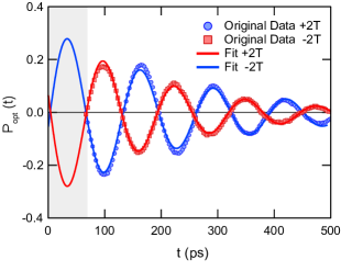
Figure 2: (Color online) Typical experimental data and fits for an excitation energy of $1.567$ eV and an excitation intensity of 6 mW. The time of laser excitation defines $t=0$. The red squares (blue circles) show the measured SQBs with an applied magnetic field of $+2$ T ($-2$ T) while the dashed lines represent the corresponding fits. Within the blue shaded area, laser straylight may influence the measured degree of polarization. Therefore, the data are fitted only outside the blue shaded area for ($t-t_{0}\geq 80$ ps).

IV Results and Discussion

IV.1 Excitation in the growth direction

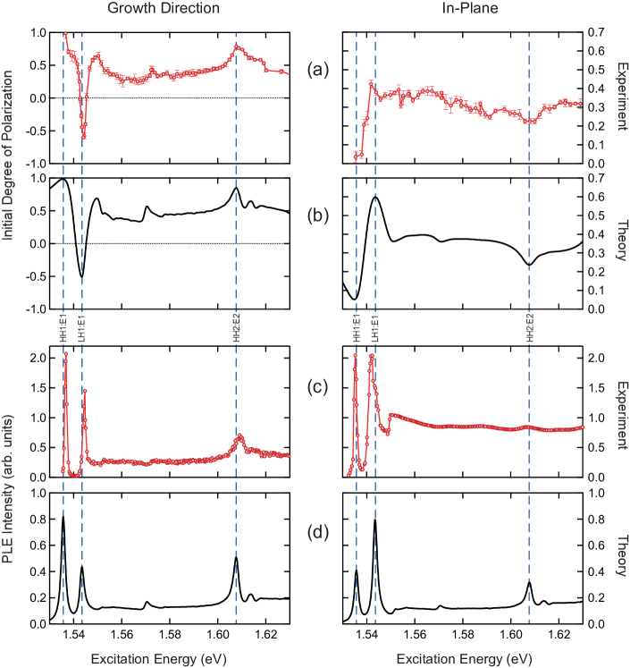
Figure 3: (Color online) Comparison of (a) the experimental results and (b) calculated values for the initial degree of electron spin polarization as a function of the excitation energy. The left (right) column shows the data for excitation in growth-direction (in the QW-plane). The lower panels show the absorption coefficient obtained from PLE- measurements (c) and theory (d) in growth direction (left) and for in-plane excitation (right).

We perform measurements of $P_{0}$ for excitation in the growth direction to characterize the sample and for comparison with the results obtained for in-plane excitation. The left column in Fig. 3 shows (a) the measured $P_{0}$, (b) the calculated $P_{0}$, and (c) the measured PL excitation (PLE) spectrum as a function of the excitation energy. We extract from the PLE spectrum a full width at half maximum (FWHM) of the lowest HH transition of $1$ meV and use this value for a phenomenological Lorentzian broadening of the numerically calculated spectrum. We briefly discuss the features of the measured $P_{0}$ going from low to high excitation energies. For resonant excitation at $1.537$ eV of the transition from the first HH subband to the first electron subband (HH1:E1), we find, as expected, $P_{0}=1$. Around the LH1:E1 transition at $1.544$ eV, we observe a sign reversal of $P_{0}$ leading to a maximum negative initial degree of spin polarization of $P_{0}\approx-0.6$. The next peak at $1.55$ eV reflects the absorption edge of the HH1:E1 exciton continuum. We find two additional peaks at $1.572$ eV and $1.61$ eV, which correspond to the HH3:E1 and HH2:E2 transition, respectively. All experimental features are well reproduced by the calculated spectra.

IV.2 In-plane excitation

The right column in Fig. 3 shows (a) the measured $P_{0}$, (b) the calculated $P_{0}$, (c) the measured PLE, and (d) the calculated PLE as a function of the excitation energy. We use for these calculations a Lorentzian broadening with an FWHM of 3 meV which is consistent with the measured PLE spectrum for in-plane excitation.

The significantly larger broadening for in-plane excitation results probably from surface effects such as local oxidation of the AlGaAs QW barriers at the cleaved surface. Moreover, our PLE measurements are noisier for in-plane excitation than for excitation in the growth direction since the PL intensity is lower. Finally, we note that we have to use a smaller laser-spot diameter for in-plane excitation so that small changes of the position of the exciting laser spot strongly change the detected PL intensity. Nonetheless, we find no indication that the measured PL signal contained contributions from the LH1:E1 transition, consistent with the fact that this transition lies about 7 meV above the HH1:E1 transition, which makes such a contribution rather unlikely.

All features in the spectrum for in-plane excitation are approximately 2 meV lower in energy than the corresponding features obtained for excitation in the growth direction. We expect that this result was caused by the position-dependent inhomogeneous strain that was unintenionally present in the sample during the low-temperature experiments, thus resulting in a small shift of the resonance energies. jag86 The sample was glued to a sample holder such that the edge used for the in-plane excitation was free-standing. Thus upon cooldown the edge might have experienced a different strain compared to the rest of the sample. We note, furthermore, that the spectra for in-plane excitation and for excitation in growth direction were measured in different cooldowns, which likewise could have resulted in different amounts of unintentional strain in these experiments.

In the PLE spectrum measured for in-plane excitation the peak attributed to the LH1:E1 exciton has an asymmetric line shape, suggesting that two excitons with almost the same energy contribute to this peak. Such a doublet structure may occur if the standard selection rules for a symmetric QW are relaxed due to the presence of a symmetry-breaking perpendicular electric field. win95a We found that for the system studied here a weak field of a few kV/cm gives rise to a second resonance slightly above the LH1:E1 resonance. For our rather sensitive setup we cannot exclude that such an electric field is present at the cleaved surface. We note that our calculations indicate that the additional resonance does not significantly affect the measured initial spin polarization $P_{0}$. The features in the spectra at higher energies are not affected either by such a weak electric field.

Again, we discuss the features of $P_{0}$ going from low to high excitation energy. For resonant excitation of the HH1:E1 transition at $1.535$ eV, we measure $P_{0}\approx 0.04$, which is close to the calculated $P_{0}$ [see Fig. 3(b)]. Our calculations show that this small but finite $P_{0}$ results from the broadening of the LH1:E1 transition and that $P_{0}$ vanishes with decreasing broadening. This is consistent with the simplified model in Sec. II which suggests that the polarization of the HH1:E1 PL in $x$ direction is always linearly polarized independent of the electron spin polarization, i.e., the PL emitted in-plane of a QW gives no indication about the electron spin polarization in the case of the HH1:E1 transition. This would be different if the LH state contributed to the PL transition, e.g., if LH and HH transitions overlapped due to broadening, if the LH states were thermally occupied, or if the LH transition were energetically below the HH transition due to strain. voi84

Figure 3(a) shows for excitation energies between $1.535$ eV and $1.542$ eV an increase in $P_{0}$ as a function of energy with a maximum of the measured $P_{0}\approx 0.43$ at the LH1:E1 transition ($1.542$ eV). Surprisingly, the measured $P_{0}$ at the LH1:E1 transition is significantly lower than the calculated value $P_{0}=0.6$. Such a difference between experiment and theory is only observed for resonant in-plane excitation of the LH transition. We discuss this point in more detail in Sec. IV.3. For excitation energies above the LH transition, $P_{0}$ is nearly constant apart from a dip at $1.608$ eV which results from the HH2:E2 transition. Contrary to the case of resonant HH1:E1 excitation, we do not obtain $P_{0}\approx 0$ since all excitons above the HH1:E1 absorption edge are Fano resonances win95a and the contribution of the LH1:E1 continuum gives rise to a nonzero $P_{0}$.

IV.3 $P_{0}$ at the LH1:E1 resonance

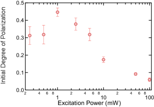
Figure 4: (Color online) $P_{0}$ as a function of the excitation energy for resonant LH1:E1 excitation at $1.542$ eV. The excitation power of $1$ mW for maximum $P_{0}$ is comparable to the excitation power used in Fig. 3.

In this section we discuss possible reasons for the reduction of the measured $P_{0}$ at the LH1:E1 transition. At first glance, spin-dependent phase-space filling of excitonic states could be a possible explanation for this behavior. For sufficiently large excitation powers $P_{\mathrm{exc}}$, the optically created electrons and holes inhibit the creation of additional carriers due to Pauli blocking. This effect is known as optical bleaching and leads to a decrease in $P_{0}$ with increasing excitation powers. To check for optical bleaching, we measure $P_{0}$ at the LH1:E1 transition as a function of $P_{\mathrm{exc}}$ (see Fig. 4). The measurements are performed with a nearly identical experimental setup but, for experimental reasons, with a picosecond laser with a spectral linewidth of $\approx 0.4$ nm FWHM. The experimental results clearly show a strong influence of phase-space filling as $P_{0}$ decreases with increasing $P_{\mathrm{exc}}$ for $P_{\mathrm{exc}}>1$ mW. However, we still measure a maximal $P_{0}\approx 0.45$ since $P_{0}$ also decreases for $P_{\mathrm{exc}}<1$ mW. Such a decrease of $P_{0}$ with decreasing excitation power has been observed before for excitation in growth direction (see Fig. 6 in Ref. pfa05, ) and has been explained by a fast initial spin relaxation, i.e., a fast excitonically induced electron spin relaxation during the thermalization process which takes place within our time resolution. We may expect that fast initial spin relaxation is particularly important for the LH1:E1 resonance because thermalization of the resonantly excited LH excitons is much slower than the nearly instantaneous thermalization of non-resonantly excited excitons in the continuum where electron-electron and electron-phonon scattering occurs on very short time scales of the order of 100 fs—consistent with the fact that only for the LH1:E1 resonance do we measure a value of $P_{0}$ that is significantly lower than theoretically expected.

The initial spin polarization $P_{0}$ may also be reduced due to an enhanced broadening of the resonance lines for in-plane excitation compared to excitation in growth direction. This can clearly be seen by comparing the PLE data for both excitation geometries: The resonances for in-plane excitation are shifted to lower energies as in the case of excitaton in growth direction (see Fig. 3). It appears that this has a large effect on the LH1:E1 transition, so that we might face an energy-dependent line broadening here. Since the broadening of the resonances (in our case approximately 3 meV) implies smaller values for the measuerd $P_{0}$, our measured data for $P_{0}$ agrees well with the measured PLE data for in-plane excitation.

V Theory

To obtain a theoretical model for the optical spin orientation, it is our goal to evaluate the spin density matrix for the optically induced electron distribution. dym76 For clarity, we will first develop the theory neglecting the Coulomb interaction between electron and hole states. Then we will introduce the modifications due to the formation of excitons.

V.1 Single-particle spectrum

The starting point of our theoretical discussion is an extension of the general theory in Ch. 5 of Ref. hau94, to multicomponent single-particle states. win03 We describe the system by means of the single-particle density operator $\rho$. We use a basis of single-particle states (electrons and holes) of the unperturbed system

$$\langle{{\bm{\mathrm{r}}}|\alpha{\bm{\mathrm{k}}}}\rangle\equiv\psi_{\alpha{\bm{\mathrm{k}}}}({\bm{\mathrm{r}}})=\sum_{n=1}^{N}\frac{e^{i{\bm{\mathrm{k}}}\cdot{\bm{\mathrm{\rho}}}}}{2\pi}\;\xi_{\alpha{\bm{\mathrm{k}}}}^{n}(z)\>u_{n{\bm{\mathrm{0}}}}({\bm{\mathrm{r}}}),$$ (8)

which are eigenfunctions of the $N\times N$ multiband Hamiltonian $H_{0}$. Here ${\bm{\mathrm{r}}}=({\bm{\mathrm{\rho}}},z)$, ${\bm{\mathrm{k}}}$ is the wave vector for the in-plane motion, and $u_{n{\bm{\mathrm{0}}}}({\bm{\mathrm{r}}})$ are the basis functions of $H_{0}$ which are Bloch functions for ${\bm{\mathrm{k}}}={\bm{\mathrm{0}}}$. The position-dependent expansion coefficents are the spinors $e^{i{\bm{\mathrm{k}}}\cdot{\bm{\mathrm{\rho}}}}\,\xi_{\alpha{\bm{\mathrm{k}}}}^{n}(z)/(2\pi)$. The energy eigenvalues corresponding to $|{\alpha{\bm{\mathrm{k}}}}\rangle$ are the subband dispersions $E_{\alpha}({\bm{\mathrm{k}}})$, i.e., $H_{0}({\bm{\mathrm{k}}})\,|{\alpha{\bm{\mathrm{k}}}}\rangle=E_{\alpha}({\bm{\mathrm{k}}})\,|{\alpha{\bm{\mathrm{k}}}}\rangle$. Now we can write $\rho$ as

$$\rho({\bm{\mathrm{k}}},t)=\sum_{\alpha,\alpha^{\prime}}\rho_{\alpha,\alpha^{\prime}}({\bm{\mathrm{k}}},t)\>|{\alpha{\bm{\mathrm{k}}}}\rangle\langle{\alpha^{\prime}{\bm{\mathrm{k}}}}|$$ (9)

with expansion coefficients $\rho_{\alpha,\alpha^{\prime}}({\bm{\mathrm{k}}},t)$. Here the sums run over both the electron subbands $\alpha_{e}$ and the hole subbands $\alpha_{h}$. Using the dipole approximation, the light field is described by scalar

$$V=\frac{e}{m_{0}}A_{0}\>\lim_{\eta\rightarrow 0}\left(e^{-i\omega t+\eta t}\>\hat{{\bm{\mathrm{e}}}}\cdot{\bm{\mathrm{p}}}+\operatorname{hc}\right)\equiv\frac{e}{m_{0}}{\bm{\mathrm{A}}}_{0}(t)\cdot{\bm{\mathrm{p}}}.$$ (10)

Here ${\bm{\mathrm{A}}}_{0}(t)$ is the vector potential for the light field, $\eta\rightarrow 0$ describes the adiabatic switching on of the perturbation $V$, and $\operatorname{hc}$ denotes the Hermitian conjugate of the preceding term. We remark that for circularly polarized light, the polarization vector $\hat{{\bm{\mathrm{e}}}}$ is complex. The first term in Eq. (10) proportional to $e^{-i\omega t}$ describes absorption, while the second term describes emission. To simplify our formulas, we neglect below all terms related with emission. Assuming that the envelope functions $e^{i{\bm{\mathrm{k}}}\cdot{\bm{\mathrm{\rho}}}}\;\xi_{\alpha{\bm{\mathrm{k}}}}^{n}(z)/(2\pi)$ are slowly varying on the length scale of the lattice constant, we obtain for the matrix elements of ${\bm{\mathrm{p}}}$ evaluated between electron and hole states

$${\bm{\mathcal{P}}}_{\alpha_{h}\alpha_{e}}({\bm{\mathrm{k}}}) = \langle{\alpha_{h}{\bm{\mathrm{k}}}|{\bm{\mathrm{p}}}|\alpha_{e}{\bm{\mathrm{k}}}}\rangle$$

$$= \sum_{n_{e},\,n_{h}}\int dz\;\xi^{n_{h}\,\ast}_{\alpha_{h}{\bm{\mathrm{k}}}}(z)\>\xi^{n_{e}}_{\alpha_{e}{\bm{\mathrm{k}}}}(z)\>\langle{u_{n_{h}}|{\bm{\mathrm{p}}}|u_{n_{e}}}\rangle.$$

We neglect matrix elements of ${\bm{\mathrm{p}}}$ in between electron states and in between hole states which would give rise to intraband optical transitions in the infrared. Then $V$ becomes

$$V({\bm{\mathrm{k}}},t)=\frac{e}{m_{0}}\sum_{\alpha_{h},\alpha_{e}}\Bigl{[}{\bm{\mathrm{A}}}_{0}(t)\cdot{\bm{\mathcal{P}}}_{\alpha_{h}\alpha_{e}}({\bm{\mathrm{k}}})\;|{\alpha_{h}{\bm{\mathrm{k}}}}\rangle\langle{\alpha_{e}{\bm{\mathrm{k}}}}|+\operatorname{hc}\Bigr{]}.$$ (12)

In the presence of the perturbation $V$, the density operator $\rho({\bm{\mathrm{k}}},t)$ obeys the Liouville equation

$$\frac{d}{dt}\rho({\bm{\mathrm{k}}},t)=\frac{i}{\hbar}\left[\rho({\bm{\mathrm{k}}},t),H_{0}({\bm{\mathrm{k}}})+V({\bm{\mathrm{k}}})\right].$$ (13)

Switching to the interaction picture (superscript $I$), this equation becomes

$$\begin{array}[b]{>{\displaystyle}r>{\displaystyle}l}\frac{d}{dt}\rho^{I}({\bm{\mathrm{k}}},t)=&\frac{ie}{\hbar\,m_{0}}\sum_{\alpha,\alpha^{\prime}}\sum_{\alpha_{h},\alpha_{e}}\rho_{\alpha,\alpha^{\prime}}^{I}({\bm{\mathrm{k}}},t)\>{\bm{\mathrm{A}}}_{0}(t)\\ \hfil&\cdot\Bigl{[}\;{\bm{\mathcal{P}}}_{\alpha_{h}\alpha_{e}}({\bm{\mathrm{k}}})\;e^{i[E_{\alpha_{h}}({\bm{\mathrm{k}}})-E_{\alpha_{e}}({\bm{\mathrm{k}}})]t/\hbar}\left(|{\alpha{\bm{\mathrm{k}}}}\rangle\langle{\alpha^{\prime}{\bm{\mathrm{k}}}|\alpha_{h}{\bm{\mathrm{k}}}}\rangle\langle{\alpha_{e}{\bm{\mathrm{k}}}}|-|{\alpha_{h}{\bm{\mathrm{k}}}}\rangle\langle{\alpha_{e}{\bm{\mathrm{k}}}|\alpha{\bm{\mathrm{k}}}}\rangle\langle{\alpha^{\prime}{\bm{\mathrm{k}}}}|\right)\\ \hfil&\hskip 3.00003pt+{\bm{\mathcal{P}}}_{\alpha_{e}\alpha_{h}}({\bm{\mathrm{k}}})\;e^{i[E_{\alpha_{e}}({\bm{\mathrm{k}}})-E_{\alpha_{h}}({\bm{\mathrm{k}}})]t/\hbar}\left(|{\alpha{\bm{\mathrm{k}}}}\rangle\langle{\alpha^{\prime}{\bm{\mathrm{k}}}|\alpha_{e}{\bm{\mathrm{k}}}}\rangle\langle{\alpha_{h}{\bm{\mathrm{k}}}}|-|{\alpha_{e}{\bm{\mathrm{k}}}}\rangle\langle{\alpha_{h}{\bm{\mathrm{k}}}|\alpha{\bm{\mathrm{k}}}}\rangle\langle{\alpha^{\prime}{\bm{\mathrm{k}}}}|\right)\Bigr{]}.\end{array}$$ (14)

As we neglected in Eq. (11) the momentum matrix elements in between electron states and in between hole states, this equation can be decomposed into separate equations for the electron, hole, and the off-diagonal electron-hole subspaces

$$\frac{d}{dt}\rho_{\alpha_{e},\alpha_{e}^{\prime}}^{I}({\bm{\mathrm{k}}},t) = \frac{ie}{\hbar\,m_{0}}{\bm{\mathrm{A}}}_{0}(t)\cdot\sum_{\alpha_{h}}\Bigl{[}{\bm{\mathcal{P}}}_{\alpha_{h}\alpha_{e}^{\prime}}({\bm{\mathrm{k}}})\>e^{-i[E_{\alpha_{e}^{\prime}}({\bm{\mathrm{k}}})-E_{\alpha_{h}}({\bm{\mathrm{k}}})]t/\hbar}\rho_{\alpha_{e},\alpha_{h}}^{I}({\bm{\mathrm{k}}},t)-{\bm{\mathcal{P}}}_{\alpha_{e}\alpha_{h}}({\bm{\mathrm{k}}})\>e^{i[E_{\alpha_{e}}({\bm{\mathrm{k}}})-E_{\alpha_{h}}({\bm{\mathrm{k}}})]t/\hbar}\rho_{\alpha_{h},\alpha_{e}^{\prime}}^{I}({\bm{\mathrm{k}}},t)\Bigr{]}$$

(15a)

$$\frac{d}{dt}\rho_{\alpha_{h},\alpha_{h}^{\prime}}^{I}({\bm{\mathrm{k}}},t) = \frac{ie}{\hbar\,m_{0}}{\bm{\mathrm{A}}}_{0}(t)\cdot\sum_{\alpha_{e}}\Bigl{[}{\bm{\mathcal{P}}}_{\alpha_{e}\alpha_{h}^{\prime}}({\bm{\mathrm{k}}})\>e^{i[E_{\alpha_{e}}({\bm{\mathrm{k}}})-E_{\alpha_{h}^{\prime}}({\bm{\mathrm{k}}})]t/\hbar}\rho_{\alpha_{h},\alpha_{e}}^{I}({\bm{\mathrm{k}}},t)-{\bm{\mathcal{P}}}_{\alpha_{h}\alpha_{e}}({\bm{\mathrm{k}}})\>e^{-i[E_{\alpha_{e}}({\bm{\mathrm{k}}})-E_{\alpha_{h}}({\bm{\mathrm{k}}})]t/\hbar}\rho_{\alpha_{e},\alpha_{h}^{\prime}}^{I}({\bm{\mathrm{k}}},t)\Bigr{]}$$

$$\frac{d}{dt}\rho_{\alpha_{e},\alpha_{h}}^{I}({\bm{\mathrm{k}}},t) = -\frac{ie}{\hbar\,m_{0}}{\bm{\mathrm{A}}}_{0}(t)\cdot{\bm{\mathcal{P}}}_{\alpha_{e}\alpha_{h}}({\bm{\mathrm{k}}})\>e^{i[E_{\alpha_{e}}({\bm{\mathrm{k}}})-E_{\alpha_{h}}({\bm{\mathrm{k}}})]t/\hbar}\left[\rho_{\alpha_{h},\alpha_{h}}^{I}({\bm{\mathrm{k}}},t)-\rho_{\alpha_{e},\alpha_{e}}^{I}({\bm{\mathrm{k}}},t)\right].$$ (15c)

In quasi equilibrium (steady state) we can solve these equations iteratively. hau94 To lowest order, the diagonal elements $\rho_{\alpha,\alpha}({\bm{\mathrm{k}}},t)$ are given by thermal (Fermi) distribution functions

$$\rho_{\alpha,\alpha}^{(0)}({\bm{\mathrm{k}}})=f_{\alpha}({\bm{\mathrm{k}}}).$$ (16)

To simplify the analysis we assume temperature $T=0$, i.e., $f_{\alpha_{h}}({\bm{\mathrm{k}}})=1$ and $f_{\alpha_{e}}({\bm{\mathrm{k}}})=0$. Now we can integrate Eq. (15c) to obtain the block off-diagonal elements of $\rho^{I}$

$$\rho_{\alpha_{e},\alpha_{h}}^{I}({\bm{\mathrm{k}}},t)=-\frac{eA_{0}}{\,m_{0}}\lim_{\eta\rightarrow 0}\frac{e^{i[E_{\alpha_{e}}({\bm{\mathrm{k}}})-E_{\alpha_{h}}({\bm{\mathrm{k}}})-\hbar\omega-i\hbar\eta]t/\hbar}}{E_{\alpha_{e}}({\bm{\mathrm{k}}})-E_{\alpha_{h}}({\bm{\mathrm{k}}})-\hbar\omega-i\hbar\eta}\;\hat{{\bm{\mathrm{e}}}}\cdot{\bm{\mathcal{P}}}_{\alpha_{e}\alpha_{h}}({\bm{\mathrm{k}}}).$$ (17)

We insert Eq. (17) into Eq. (15a). Integrating the resulting equation and going back to the Schrödinger picture we get dym76

$$\rho_{\alpha_{e},\alpha_{e}^{\prime}}({\bm{\mathrm{k}}},t)=\frac{e^{2}A_{0}^{2}}{m_{0}^{2}}\sum_{\alpha_{h}}\;\lim_{\eta\rightarrow 0}\>\frac{[\hat{{\bm{\mathrm{e}}}}\cdot{\bm{\mathcal{P}}}_{\alpha_{e}\alpha_{h}}({\bm{\mathrm{k}}})]\,[\hat{{\bm{\mathrm{e}}}}^{\ast}\cdot{\bm{\mathcal{P}}}_{\alpha_{h}\alpha_{e}^{\prime}}({\bm{\mathrm{k}}})]\;e^{2\eta t}}{[E_{\alpha_{e}}({\bm{\mathrm{k}}})-E_{\alpha_{h}}({\bm{\mathrm{k}}})-\hbar\omega+i\hbar\eta]\,[E_{\alpha_{e}^{\prime}}({\bm{\mathrm{k}}})-E_{\alpha_{h}}({\bm{\mathrm{k}}})-\hbar\omega-i\hbar\eta]}.$$ (18)

For the resonant case $E_{\alpha_{e}}({\bm{\mathrm{k}}})-E_{\alpha_{h}}({\bm{\mathrm{k}}})=\hbar\omega$ the limit $\eta\rightarrow 0$ is ill-defined. Yet we have

$$\frac{d}{dt}\;\rho_{\alpha_{e},\alpha_{e}}({\bm{\mathrm{k}}},t)\equiv\dot{\rho}_{\alpha_{e},\alpha_{e}}({\bm{\mathrm{k}}},t)=\frac{2\pi}{\hbar}\,\frac{e^{2}A_{0}^{2}}{m_{0}^{2}}\sum_{\alpha_{h}}\left|\hat{{\bm{\mathrm{e}}}}\cdot{\bm{\mathcal{P}}}_{\alpha_{e}\alpha_{h}}({\bm{\mathrm{k}}})\right|^{2}\;\delta[E_{\alpha_{e}}({\bm{\mathrm{k}}})-E_{\alpha_{h}}({\bm{\mathrm{k}}})-\hbar\omega]$$ (19)

and the (dimensionless) absorption coefficient reads

$$\alpha(\omega) = \frac{e^{2}}{4\pi\epsilon_{0}\,\hbar c}\,\frac{4\pi}{n}\,\frac{m_{0}}{e^{2}A_{0}^{2}\,\omega}\operatorname{tr}\dot{\rho}(\omega)$$ (20a)

$$= \frac{\alpha_{0}}{\hbar\omega\,m_{0}}\sum_{\alpha_{e},\alpha_{h}}\int\!\frac{d^{2}k}{(2\pi)^{2}}\>\left|\hat{{\bm{\mathrm{e}}}}\cdot{\bm{\mathcal{P}}}_{\alpha_{e}\alpha_{h}}({\bm{\mathrm{k}}})\right|^{2}\;\delta[E_{\alpha_{e}}({\bm{\mathrm{k}}})-E_{\alpha_{h}}({\bm{\mathrm{k}}})-\hbar\omega],$$ (20b)

where the trace runs over all electron states and

$$\alpha_{0}\equiv\frac{e^{2}}{4\pi\epsilon_{0}\,\hbar c}\,\frac{8\pi^{2}}{n}$$ (21)

with $\epsilon_{0}$ the permittivity of free space, $c$ the speed of light and $n$ the index of refraction.

Finally, we obtain for the matrix elements $\varrho_{n_{e},n_{e}^{\prime}}(\omega)$ of the electron spinor density matrix $\varrho$

$$\varrho_{n_{e},n_{e}^{\prime}}(\omega)=\frac{e^{2}A_{0}^{2}}{m_{0}^{2}}\sum_{\alpha_{e},\alpha_{e}^{\prime}}\int\!dz_{e}\;\xi^{n_{e}\,\ast}_{\alpha_{e}{\bm{\mathrm{k}}}}(z_{e})\>\xi^{n_{e}^{\prime}}_{\alpha_{e}^{\prime}{\bm{\mathrm{k}}}}(z_{e})\sum_{\alpha_{h}}\int\!\frac{d^{2}k}{(2\pi)^{2}}\>\frac{[\hat{{\bm{\mathrm{e}}}}\cdot{\bm{\mathcal{P}}}_{\alpha_{e}\alpha_{h}}({\bm{\mathrm{k}}})]\,[\hat{{\bm{\mathrm{e}}}}^{\ast}\cdot{\bm{\mathcal{P}}}_{\alpha_{h}\alpha_{e}^{\prime}}({\bm{\mathrm{k}}})]\;e^{2\eta t}}{[E_{\alpha_{e}}({\bm{\mathrm{k}}})-E_{\alpha_{h}}({\bm{\mathrm{k}}})-\hbar\omega+i\hbar\eta]\,[E_{\alpha_{e}^{\prime}}({\bm{\mathrm{k}}})-E_{\alpha_{h}}({\bm{\mathrm{k}}})-\hbar\omega-i\hbar\eta]}$$ (22)

and the spin polarization induced by a steady-state optical excitation is given by

$${\bm{\mathrm{P}}}(\omega)=\frac{\operatorname{tr}\left[{\bm{\mathrm{S}}}\,\varrho(\omega)\right]}{\operatorname{tr}\varrho(\omega)}=\frac{\operatorname{tr}\left[{\bm{\mathrm{S}}}\,\dot{\varrho}(\omega)\right]}{\operatorname{tr}\dot{\varrho}(\omega)}\>,$$ (23)

i.e., while the density matrices $\rho$ and $\varrho$ are ill-defined in the limit $\eta\rightarrow 0$, the expectation values of observables are well-defined and independent of $t$. (Yet we keep $\eta>0$ to simulate a finite broadening of the energy levels.) The second equality in Eq. (23) indicates that ${\bm{\mathrm{P}}}(\omega)$ is, indeed, equivalent to the definition of the spin polarization proposed previously. pfa05 The generalized spin matrices ${\bm{\mathrm{S}}}$ are defined in Eq. (6.65) of Ref. win03, .

V.2 Excitonic spectrum

We can extend the theory developed in the previous subsection to take into account the Coulomb interaction between electron and hole states, thus giving rise to the formation of excitons. For this purpose, we use the accurate exciton theory described in Ref. win95a, . It is based on an axial approximation for $H_{0}$, so that total angular momentum $l$ is a good quantum number. We expand the exciton states in terms of the single-particle states (8)

$$\Psi_{l\gamma}({\bm{\mathrm{r}}}_{e},{\bm{\mathrm{r}}}_{h})=\frac{1}{(2\pi)^{3/2}}\sum_{\alpha_{e},\,\alpha_{h}}\sum_{n_{e},\,n_{h}}\int d^{2}k\>\phi_{l\gamma\,k}^{\alpha_{e}\alpha_{h}}\>e^{i{\bm{\mathrm{k}}}\cdot({\bm{\mathrm{\rho}}}_{e}-{\bm{\mathrm{\rho}}}_{h})}\>e^{i(l-M_{n_{e}}+M_{n_{h}})\varphi}\>\xi^{n_{e}}_{\alpha_{e}k}(z_{e})\,u_{n_{e}{\bm{\mathrm{0}}}}({\bm{\mathrm{r}}}_{e})\left[\xi^{n_{h}}_{\alpha_{h}k}(z_{h})\,u_{n_{h}{\bm{\mathrm{0}}}}({\bm{\mathrm{r}}}_{h})\right]^{\ast}$$ (24)

with expansion coefficients $e^{il\varphi}\phi_{l\gamma\,k}^{\alpha_{e}\alpha_{h}}$ and ${\bm{\mathrm{k}}}=(k,\varphi)$. Similar to Eq. (22), we obtain for the matrix elements $\varrho_{n_{e},n_{e}^{\prime}}(\omega)$ of the electron spinor density matrix $\varrho$

$$\varrho_{n_{e},n_{e}^{\prime}}(\omega)=\frac{e^{2}A_{0}^{2}}{m_{0}^{2}}\>\sum_{l,l^{\prime}}\sum_{\gamma,\gamma^{\prime}}\>\frac{[\hat{{\bm{\mathrm{e}}}}\cdot{\bm{\mathcal{P}}}_{l\gamma}^{\ast}]\,[\hat{{\bm{\mathrm{e}}}}^{\ast}\cdot{\bm{\mathcal{P}}}_{l^{\prime}\gamma^{\prime}}]\;e^{2\eta t}}{[E_{l\gamma}-\hbar\omega+i\hbar\eta]\,[E_{l^{\prime}\gamma^{\prime}}-\hbar\omega-i\hbar\eta]}\sum_{\alpha_{e},\alpha_{e}^{\prime}}\sum_{\alpha_{h}}\int\!dk\,k\;\phi_{l\gamma\,k}^{\alpha_{e}\alpha_{h}\ast}\>\phi_{l^{\prime}\gamma^{\prime}\,k}^{\alpha_{e}^{\prime}\alpha_{h}}\>\int\!dz_{e}\;\xi^{n_{e}\,\ast}_{\alpha_{e}k}(z_{e})\>\xi^{n_{e}^{\prime}}_{\alpha_{e}^{\prime}k}(z_{e})\>,$$ (25a)

where

$${\bm{\mathcal{P}}}_{l\gamma}=\sqrt{\frac{\mathcal{A}}{2\pi}}\sum_{\alpha_{e},\,\alpha_{h}}\sum_{n_{e},\,n_{h}}\int\!dk\,k\;\phi_{l\gamma\,k}^{\alpha_{e}\alpha_{h}}\>\delta_{l-M_{n_{e}}+M_{n_{h}},\,0}\;\int\!dz\;\xi^{n_{h}\,\ast}_{\alpha_{h}k}(z)\>\xi^{n_{e}}_{\alpha_{e}k}(z)\>\langle{u_{n_{h}}|{\bm{\mathrm{p}}}\,|u_{n_{e}}}\rangle$$ (25b)

are the dipole matrix elements of the exciton states with $\mathcal{A}$ the area of the QW interface. Once again, the absorption coefficient is given by Eq. (20) (note $\operatorname{tr}\rho=\operatorname{tr}\varrho$), and the optically induced spin polarization is given by Eq. (23). These equations describe optical absorption and the resulting spin polarization for arbitrary polarization directions $\hat{{\bm{\mathrm{e}}}}$ of the exciting light field.

V.3 Kane Model

For all numerical calculations presented in this work we have used for the multiband Hamiltonian $H_{0}$ the $8\times 8$ Kane Hamiltonian for the lowest conduction band $\Gamma_{6}^{c}$, the topmost valence band $\Gamma_{8}^{v}$ and the spin split-off valence band $\Gamma_{7}^{v}$ including remote-band contributions of second order in $k$. This Hamiltonian has been discussed in detail, e.g., in Ref. win03, . It is known to provide an accurate description of all important details of the semiconductor band structure including the nonparabolic dispersion and the mixing of HH and LH states. win95a ; pfa05 The numerical values for all band structure parameters were likewise taken from Ref. win03, . The calculations were carried out using the nominal growth parameters without any fitting parameters. The tiny differences in energetic positions of the peaks in the measured and calculated spectra in Fig. 3 probably result from the uncertainty in the Al concentration of the QW barriers.

Within the Kane model, we readily obtain Eq. (1) from Eq. (22) if we neglect the in-plane dispersion of the electron and hole states (i.e., in-plane wave vector ${\bm{\mathrm{k}}}=0$) as well as the ${\bm{\mathrm{k}}}\cdot{\bm{\mathrm{p}}}$ coupling between conduction and valence band states so that all subband states are represented by their dominant spinor component.

V.4 Discussion

The calculated spectra presented in Figs. 3(b) and (d) based on the excitonic model of Sec. V.2 are overall in good agreement with the measured spectra in Figs. 3(a) and (c). The simplified model from Sec. II neglecting Coulomb coupling and HH-LH mixing suggests that individual peaks in the spectra can be attributed to pairs of one electron and one hole subband. As discussed in more detail in Refs. pfa05, and win95a, , such an approximate model is best justified for the discrete excitonic states below the excitonic continuum. In the excitonic continuum the excitons become Fano resonances fan61 that are strongly modified by Coulomb coupling and HH-LH mixing of individual subbands. These effects are immediately visible in the calculated spectrum of Figs. 3(b) (right column). Here the spin polarization associated with the discrete HH1:E1 exciton is close to zero, as expected based on the model of Sec. II (being nonzero only because of the finite broadening of the LH1:E1 exciton). On the other hand, the dip of the polarization at the energy of the HH2:E2 exciton is essentially independent of the phenomenological broadening, but it reflects the finite width of a Fano resonance. win95a ; fan61

VI Conclusion

The comparison of the results for excitation in the growth direction and in-plane excitation clearly shows the dependence of the optical selection rules on the excitation and detection geometry. Instead of $P_{0}=1$ for excitation in the growth direction at the HH1:E1 resonance, we find $P_{0}\approx 0$ for excitation in $y$-direction. Moreover, we find no traces of a sign reversal in our data, i. e., there is no region with $P_{0}\approx 0$ except for resonant HH1:E1 excitation. Such a sign reversal is typical for excitation in the growth direction with energies close to the LH1:E1 resonance.

The experiments are well described by an accurate model for the spin density matrix induced by the optical excitation. This model takes into account both the effects of the semiconductor band structure such as HH-LH coupling and nonparabolicity, and the Coulomb coupling between electron and hole states giving rise to the formation of excitons.

- (1) I. Žutić, J. Fabian, and S. Das Sarma, Rev. Mod. Phys. 76, 323 (2004).
- (2) M. I. Dyakonov and V. I. Perel, in Optical Orientation, edited by F. Meier and B. P. Zakharchenya (Elsevier, Amsterdam, 1984), pp. 11–71.
- (3) D. Hägele, M. Oestreich, W. W. Rühle, N. Nestle, and K. Eberl, Appl. Phys. Lett. 73, 1580 (1998).
- (4) S. A. Crooker and D. L. Smith, Phys. Rev. Lett. 94, 236601 (2005).
- (5) A. M. Gilinsky, A. Winter, C. Mejía-García, H. Pascher, K. S. Zhuravlev, A. V. Efanov, E. V. Kozhemyakina, A. Amo, and L. Viña, Europhys. Lett. 88, 17001 (2009).
- (6) S. D. Ganichev, P. Schneider, V. V. Bel’kov, E. L. Ivchenko, S. A. Tarasenko, W. Wegscheider, D. Weiss, D. Schuh, B. N. Murdin, P. J. Phillips, et al., Phys. Rev. B 68, 081302 (2003).
- (7) M. Oestreich, J. Hübner, D. Hägele, P. J. Klar, W. Heimbrodt, W. W. Rühle, D. E. Ashenford, and B. Lunn, Appl. Phys. Lett. 74, 1251 (1999).
- (8) R. Fiederling, M. Keim, G. Reuscher, W. Ossau, G. Schmidt, A. Waag, and L. W. Molenkamp, Nature 402, 787 (1999).
- (9) B. T. Jonker, Y. D. Park, B. R. Bennett, H. D. Cheong, G. Kioseoglou, and A. Petrou, Phys. Rev. B 62, 8180 (2000).
- (10) T. C. Damen, L. Viña, J. E. Cunningham, J. Shah, and L. J. Sham, Phys. Rev. Lett. 67, 3432 (1991).
- (11) D. J. Hilton and C. L. Tang, Phys. Rev. Lett. 89, 146601 (2002).
- (12) T. Korn, M. Kugler, M. Griesbeck, R. Schulz, A. Wagner, M. Hirmer, C. Gerl, D. Schuh, W. Wegscheider, and C. Schüller, New J. Phys. 12, 043003 (2010).
- (13) S. Priyadarshi, A. M. Racu, K. Pierz, U. Siegner, M. Bieler, H. T. Duc, J. Förstner, and T. Meier, Phys. Rev. Lett. 104, 217401 (2010).
- (14) S. Pfalz, R. Winkler, T. Nowitzki, D. Reuter, A. D. Wieck, D. Hägele, and M. Oestreich, Phys. Rev. B 71, 165305 (2005).
- (15) Y. Ohno, D. K. Young, B. Beschoten, F. Matsukura, H. Ohno, and D. D. Awschalom, Nature 402, 790 (1999).
- (16) M. Oestreich, Nature 402, 735 (1999).
- (17) M. Oestreich, D. Hägele, H. C. Schneider, A. Knorr, A. Hansch, S. Hallstein, K. H. Schmidt, K. Köhler, S. W. Koch, and W. W. Rühle, Solid State Commun. 108, 753 (1998).
- (18) Throughout we define the scalar product as .
- (19) R. Winkler, Spin-Orbit Coupling Effects in Two-Dimensional Electron and Hole Systems (Springer, Berlin, 2003).
- (20) V. D. Dymnikov, M. I. D’yakonov, and N. I. Perel’, Sov. Phys.–JETP 44, 1252 (1976).
- (21) R. Fiederling, P. Grabs, W. Ossau, G. Schmidt, and L. W. Molenkamp, Appl. Phys. Lett. 82, 2160 (2003).
- (22) M. Oestreich, J. Rudolph, R. Winkler, and D. Hägele, Superlatt. Microstruct. 37, 306 (2005).
- (23) R. Lövenich, C. W. Lai, D. Hägele, D. S. Chemla, and W. Schäfer, Phys. Rev. B 66, 045306 (2002).
- (24) C. Jagannath, E. S. Koteles, J. Lee, Y. J. Chen, B. S. Elman, and J. Y. Chi, Phys. Rev. B 34, 7027 (1986).
- (25) R. Winkler, Phys. Rev. B 51, 14395 (1995).
- (26) P. Voisin, C. Delalande, M. Voos, L. L. Chang, A. Segmuller, C. A. Chang, and L. Esaki, Phys. Rev. B 30, 2276 (1984).
- (27) H. Haug and S. W. Koch, Quantum Theory of the Optical and Electronic Properties of Semiconductors (World Scientific, Singapore, 1994), 3rd ed.
- (28) U. Fano, Phys. Rev. 124, 1866 (1961).