Entanglement in a three spin system controlled by electric and magnetic fields

Abstract

We study the effect of electric field and magnetic flux on spin entanglement in an artificial triangular molecule built of coherently coupled quantum dots. In a subspace of doublet states an explicit relation of concurrence with spin correlation functions and chirality is presented. The electric field modifies super-exchange correlations, shifts many-electron levels (the Stark effect) as well as changes spin correlations. For some specific orientation of the electric field one can observe monogamy, for which one of the spins is separated from two others. Moreover, the Stark effect manifests itself in a different spin entanglement for small and strong electric fields. A role of magnetic flux is opposite, it leads to circulation of spin supercurrents and spin delocalization.

I Introduction

The last decade has seen a great interest in application of concepts from quantum information theory, for example entanglement horodeccy , to condensed matter theory amico . Since entanglement represents unique quantum correlations, the concept has been applied to exploration of phenomena in strongly correlated many-fermion systems in order to gain insight into the nature of quantum phase transitions. In this paper we show how entanglement is related with a spin correlation function and how it can be controlled by an external electric and magnetic field. We choose a system of three coherently coupled semiconducting quantum dots with three electrons, because it can be viewed as a realization of a three qubit system, which has recently been of great interest barenco ; burkard ; vinzenzo ; Weinstein ; yang . In such the system one can find two classes of truly three-partite entangled states, represented by the Greenberger-Horne-Zeilinger (GHZ) and the Werner (W) states horodeccy ; dur . Recently there are attempts to measure and control these states dicarlo , as well as to apply them in logical gates neeley . In this paper we follow a scheme for universal quantum computations, proposed by Di Vincenzo et al. vinzenzo for a spin system with exchange interactions in quantum dots, in which logical qubits are encoded in the doublet subspace with $S_{z}=+1/2$ (see also Weinstein ).

Recent experiments demonstrate that in three quantum dots one can perform coherent spin manipulations laird10 ; takakura ; gaudreu . It is well known that spin manipulation can be controlled by electric field, for example in the systems with the spin-orbit interactions kato ; golovach , by applying inhomogeneous static magnetic field laird ; pioro , by a light-induced magnetic field through the dynamical Stark effect gupta or Raman transitions imamoglu (see also hanson ). In our approach a role of the electric field is different, it modifies super-exchange coupling. In the system with a triangular geometry the electric field breaks its symmetry and changes the quantum correlations between spins. Role of a magnetic flux is different, it induces spin supercurrents flowing around the triangular ring and is the main decoherence source in that kind of systems choi . One can expect that the magnetic flux acts destructively on the entanglement.

The paper is organized as follows. In Sec. II we show that the concurrence, as a measure of entanglement, has an explicit relation with spin correlation functions and chirality in the triple spin system. Therefore one can have a simple interpretation of separability, monogamy and dark spin states. Sec. III describes our system within the Hubbard model and its canonical transformation to the Heisenberg Hamiltonian. We show that the electric field breaks the symmetry of the system and modifies exchange coupling, whereas the magnetic flux generates spin chirality. Detail studies of the concurrence, as well as the spin correlation functions and spin chirality, are presented in Sec. IV. For a special orientation of the electric field we find a biseparable state (monogamy). Sec. V summarizes the paper.

II Spin correlation functions and measure of entanglement

We begin defining wave functions for three electrons in the three qubit system. These functions can be constructed by adding a third electron to the singlet or triplet state (see pauncz ). Two spin subspaces are possible to define: quadruplets and doublets. The quadruplets are the states with the quantum spin number $S=3/2$, $S_{z}=\{\pm 3/2,\pm 1/2\}$ and the corresponding wave functions are constructed from a triplet state in the form:

$$|Q_{-3/2}\rangle=c_{3\downarrow}^{\dagger}c_{2\downarrow}^{\dagger}c_{1\downarrow}^{\dagger}|0\rangle,$$

$$|Q_{-1/2}\rangle=\frac{1}{\sqrt{3}}(c_{3\uparrow}^{\dagger}c_{2\downarrow}^{\dagger}c_{1\downarrow}^{\dagger}+c_{3\downarrow}^{\dagger}c_{2\uparrow}^{\dagger}c_{1\downarrow}^{\dagger}+c_{3\downarrow}^{\dagger}c_{2\downarrow}^{\dagger}c_{1\uparrow}^{\dagger})|0\rangle,$$

$$|Q_{1/2}\rangle=\frac{1}{\sqrt{3}}(c_{3\downarrow}^{\dagger}c_{2\uparrow}^{\dagger}c_{1\uparrow}^{\dagger}+c_{3\uparrow}^{\dagger}c_{2\downarrow}^{\dagger}c_{1\uparrow}^{\dagger}+c_{3\uparrow}^{\dagger}c_{2\uparrow}^{\dagger}c_{1\downarrow}^{\dagger})|0\rangle,$$

$$|Q_{3/2}\rangle=c_{3\uparrow}^{\dagger}c_{2\uparrow}^{\dagger}c_{1\uparrow}^{\dagger}|0\rangle.$$

Symbols $c_{i\sigma}^{\dagger}$ are creation operators of an electron with the spin $\sigma$ in the qubit i acting on the vacuum $|0\rangle$. A linear combination $|GHZ\rangle=\frac{1}{\sqrt{2}}(|Q_{-3/2}\rangle+|Q_{+3/2}\rangle)$ is known as the GHZ state. Two other functions $|Q_{+1/2}\rangle$ and $|Q_{-1/2}\rangle$ are called W-states. These states are well known in the literature dur ; wang ; miyake ; horodeccy ; amico .

In this paper the studies are focused on the doublet subspace with the total spin $S=1/2$. These states were proposed for exchange-interaction universal quantum computations vinzenzo ; Weinstein ; yang . In many cases, as the one considered in the next part of the paper, the doublet is the ground state. We assume that the system is kept coherent for a time sufficiently long in order to perform an entanglement measurement, and we fix the z-component of the total spin $S_{z}=+1/2$ in further considerations. The wave function can be expressed as

$$|\Psi_{D_{1/2}}\rangle=\alpha_{1}|D_{1/2}\rangle_{1}+\alpha_{2}|D_{1/2}\rangle_{2},$$ (1)

where:

$$|D_{1/2}\rangle_{1}=\frac{1}{\sqrt{2}}(c_{3\downarrow}^{\dagger}c_{2\uparrow}^{\dagger}-c_{3\uparrow}^{\dagger}c_{2\downarrow}^{\dagger})c_{1\uparrow}^{\dagger}|0\rangle,$$ (2)

$$|D_{1/2}\rangle_{2}=\frac{1}{\sqrt{6}}[(c_{3\downarrow}^{\dagger}c_{2\uparrow}^{\dagger}+c_{3\uparrow}^{\dagger}c_{2\downarrow}^{\dagger})c_{1\uparrow}^{\dagger}-2c_{3\uparrow}^{\dagger}c_{2\uparrow}^{\dagger}c_{1\downarrow}^{\dagger}]|0\rangle,$$ (3)

In general $|\Psi_{D_{1/2}}\rangle$ should be expanded including a linear combination with the states with double site occupation: $c_{i\uparrow}^{\dagger}c_{j\uparrow}^{\dagger}c_{j\downarrow}^{\dagger}|0\rangle$. The state $|D_{1/2}\rangle_{1}$ is prepared by adding third electron to the singlet state, whereas $|D_{1/2}\rangle_{2}$ can be prepared from triplet or singlet states pauncz . This construction allows us for gaining insight into monogamy and biseparability Acin ; Sabin .

As a measure of the entanglement we take the concurrence. In order to calculate it coffman , we define a reduced density matrix of a pair of electrons in the quantum dots $i$ and $j$: $\varrho_{ij}=\text{Tr}_{k}\varrho$, where $i$, $j$ and $k$ denote different quantum dots, and $\varrho$ is a density matrix $\varrho=|\Psi_{D}\rangle\langle\Psi_{D}|$ for the doublet subspace. Next we derive a matrix:

$$R_{ij}=\varrho_{ij}(\sigma_{y}\otimes\sigma_{y})\varrho^{\ast}_{ij}(\sigma_{y}\otimes\sigma_{y}),$$ (4)

where $\sigma_{y}$ is a Pauli matrix and the asterisk denotes complex conjugation of $\varrho_{ij}$. The concurrence is calculated as:

$$C_{ij}=\max\{0,\lambda_{1}-\lambda_{2}-\lambda_{3}-\lambda_{4}\},$$ (5)

where $\lambda_{1}$, $\lambda_{2}$, $\lambda_{3}$, $\lambda_{4}$ are square roots of eigenvalues of $R_{ij}$ in descending order. $C_{ij}$ can take values between zero (for separate states) and one (for fully quantumly entanglement states). Using this definition one can calculate the concurrence for the doublet representation (1):

$$C_{12}=\frac{2}{3}|\alpha_{2}||\sqrt{3}\alpha_{1}+\alpha_{2}|,$$ (6)

$$C_{13}=\frac{2}{3}|\alpha_{2}||\sqrt{3}\alpha_{1}-\alpha_{2}|,$$ (7)

$$C_{23}=\frac{1}{3}|3\alpha_{1}^{2}-\alpha_{2}^{2}|.$$ (8)

Let us now calculate spin correlation functions in the doublet subspace (1):

$$\langle\mathbf{S}_{1}\cdot\mathbf{S}_{2}\rangle=\frac{1}{4}[-\sqrt{3}(\alpha_{1}\alpha_{2}^{*}+\alpha_{1}^{*}\alpha_{2})-2|\alpha_{2}|^{2}],$$ (9)

$$\langle\mathbf{S}_{1}\cdot\mathbf{S}_{3}\rangle=\frac{1}{4}[\sqrt{3}(\alpha_{1}\alpha_{2}^{*}+\alpha_{1}^{*}\alpha_{2})-2|\alpha_{2}|^{2}],$$ (10)

$$\langle\mathbf{S}_{2}\cdot\mathbf{S}_{3}\rangle=\frac{1}{4}(-3|\alpha_{1}|^{2}+|\alpha_{2}|^{2}).$$ (11)

In general the coefficients $\alpha_{1}$ and $\alpha_{2}$ can be complex, for example in the presence of the magnetic flux. We show later that in this case a spin supercurrent occurs with a nonzero value of chirality

$$\langle\mathbf{S}_{1}\cdot(\mathbf{S}_{2}\times\mathbf{S}_{3})\rangle=\text{i}\frac{\sqrt{3}}{4}(\alpha_{1}\alpha_{2}^{*}-\alpha_{1}^{*}\alpha_{2}).$$ (12)

Comparing these results with the concurrence $C_{ij}$ (6)-(8) one can find, after some algebra, the following relation:

$$C_{ij}=\frac{4}{3}|\langle\mathbf{S}_{i}\cdot\mathbf{S}_{j}+\text{i}\;\mathbf{S}_{1}\cdot(\mathbf{S}_{2}\times\mathbf{S}_{3})\rangle|.$$ (13)

This fact allows us to propose the expectation value of spin correlation functions and chirality as an alternative measure of the entanglement.

In a multi-qubit system it is interesting to define monogamy of entanglement. If two qubits are fully quantumly entanglement then they cannot be correlated with the third one bennett . In this case one says about monogamy, which expresses the nonshareability of entanglement. For a three qubit system monogamy can be measured by the concurrence $C_{i(jk)}$ between a qubit i and other qubits $j,k$, which is given by the one-tangle $C^{2}_{i(jk)}=4\det\varrho_{i}$, where $\varrho_{i}=\text{Tr}_{jk}\varrho$. For biseparable states $C^{2}_{i(jk)}=0$, which means that the qubits $j$ and $k$ are fully quantumly entanglement whereas the qubit $i$ is separated. This quantity is related with the linear entropy $S_{L}(\varrho_{i})\equiv 2[1-\text{Tr}(\varrho^{2}_{i})]=4\det\varrho_{i}$. Monogamy of entanglement satisfies the relation

$$C_{i(jk)}^{2}\geq C_{ij}^{2}+C_{ik}^{2}$$ (14)

proved by Coffman, Kundu and Wooters coffman . For our case, in the doublet subspace, we have the equality $C_{i(jk)}^{2}=C_{ij}^{2}+C_{ik}^{2}$, as one could expect for pure states.

III Model of correlated spins on a triangular system of quantum dots

In this section we would like to present a specific three qubit example, namely an artificial triangular molecule built of coherently coupled semiconducting quantum dots. We show first that an external electric field and a magnetic flux can modify spin states, and later, in the next section, how these external fields influence the entanglement between spins.

Our system of three quantum dots (Fig.1) is described by the Hubbard model

$$\begin{split}\hat{H}&=\sum_{i,\sigma}\{\epsilon_{i}+Eer\cos[\theta+(i-1)2\pi/3]\}n_{i\sigma}\\ &+t\sum_{i\neq j,\sigma}(e^{i\phi/3}c_{i\sigma}^{\dagger}c_{j\sigma}+h.c.)+U\sum_{i}n_{i\downarrow}n_{i\uparrow}.\end{split}$$ (15)

Here, $\widetilde{\epsilon}_{i}=\epsilon_{i}+Eer\cos[\theta+(i-1)2\pi/3]$ corresponds to a shift of a local single electron level $\epsilon_{i}$ in the electric field $\mathbf{E}$. The polarization energy $\mathbf{E}\cdot\mathbf{P}=e\sum_{i\sigma}\mathbf{E}\cdot\mathbf{r_{i}}n_{i\sigma}=Eer\sum_{i\sigma}\cos{[\theta+(i-1)2\pi/3]}n_{i\sigma}$, where: e - the electron charge, $\mathbf{r}_{i}$ denotes a vector of the i-qubit position and $\theta$ is an angle between $\mathbf{r}_{1}$ and $\mathbf{E}$, $n_{i\sigma}$ - an electron number operator. Later for simplicity we put $\epsilon_{i}=0$ and denote $g_{E}=Eer$. The second term in (15) describes electron hopping between nearest quantum dots in the presence of the magnetic flux $\Phi$ enclosed in the triangle. According to the Peierls scaling an electron gains during hopping a phase shift $\phi=2\pi\Phi/(hc/e)$. The Coulomb onsite interaction of electrons on the quantum dots is included in the last term.

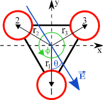
Figure 1: Model of a system of Three Quantum Dots placed in an external electric filed $\mathbf{E}$ and a magnetic flux $\Phi$.

Using this model we can calculate all properties of the system numerically. In particular for three electrons we calculate the spin correlation functions as well as the concurrence and influence of the electric field as well as the magnetic flux. To understand the results we use a canonical transformation bulka1 of the Hubbard Hamiltonian (15) to an effective Heisenberg Hamiltonian. Taking the hopping integral $t$ and the electric field $g_{E}$ as small parameters with respect to the Coulomb interaction $U$, one can get the effective Heisenberg Hamiltonian kostyrko ; dassarma :

$$\hat{H}_{\text{eff}}=\sum_{i<j}J_{ij}(\mathbf{S}_{i}\cdot\mathbf{S}_{j}-\frac{1}{4})+J_{\chi}\;\mathbf{S}_{1}\cdot(\mathbf{S}_{2}\times\mathbf{S}_{3}).$$ (16)

The first term describes the superexchange coupling between spins, for which the exchange parameter $J_{ij}$ can be calculated to the third order in $t/U$ kostyrko

$$J_{ij} = 2|t_{ij}|^{2}(\Delta_{ji}^{-1}+\Delta_{ji}^{-1})+\left(t_{ji}t_{ik}t_{kj}+t_{ji}^{*}t_{ik}^{*}t_{kj}^{*}\right)\times$$ (17)

$$(\Delta^{-1}_{ij}\Delta^{-1}_{kj}+\Delta^{-1}_{ji}\Delta^{-1}_{ki}+\Delta^{-1}_{ki}\Delta^{-1}_{kj}$$

$$-\Delta^{-1}_{ji}\Delta^{-1}_{jk}-\Delta^{-1}_{ij}\Delta^{-1}_{ik}-\Delta^{-1}_{ik}\Delta^{-1}_{jk})\,,$$

where $\Delta_{ij}=(U+\widetilde{\epsilon}_{j}-\widetilde{\epsilon}_{i})$. In the limit $g_{E}\ll U$ one can get an explicit form of $J_{ij}$:

$$J_{12}=\frac{4t^{2}}{U}+\frac{3t^{2}g_{E}^{2}(2+\cos{2\theta}+\sqrt{3}\sin{2\theta})}{U^{3}}$$

$$-\frac{12t^{3}\cos\phi\;g_{E}(\cos{\theta}-\sqrt{3}\sin{\theta})}{U^{3}},$$ (18)

$$J_{13}=\frac{4t^{2}}{U}+\frac{3t^{2}g_{E}^{2}(2+\cos{2\theta}-\sqrt{3}\sin{2\theta})}{U^{3}}$$

$$-\frac{12t^{3}\cos\phi\;g_{E}(\cos{\theta}+\sqrt{3}\sin{\theta})}{U^{3}},$$ (19)

$$J_{23}=\frac{4t^{2}}{U}+\frac{6t^{2}g_{E}^{2}(1-\cos{2\theta})}{U^{3}}+\frac{24t^{3}\cos\phi\;g_{E}\cos{\theta}}{U^{3}}.$$ (20)

One can see that the second term is proportional to $g_{E}^{2}$ and corresponds to the quadratic Stark effect. When the electric field rotates, this term leads to oscillations with the period $\pi$. The linear Stark effect is described by the third term, which corresponds to the period of oscillations equal to $2\pi$. The linear term in $J_{23}$ is always positive, whereas for $J_{12}$ and $J_{13}$ the linear terms can be negative. At $\theta=0$ one can see that $J_{23}$ increases linearly with $g_{E}$, whereas the couplings $J_{12}=J_{13}$ and they first decrease, and next increase quadratically for a larger $g_{E}$. At $g_{E}=4t\cos\phi$ we get $J_{12}=J_{13}=J_{23}$ and the system becomes uniform once again.

The second term in the effective Hamiltonian (16) describes chirality of electrons in the presence of the magnetic flux. The term is connected with the Aharonov-Bohm effect and with the persistent currents moving around the flux enclosed by the three quantum dot ring. The coupling parameter calculated to the third order in $t/U$ is given by kostyrko

$$J_{\chi}=-\textsl{i}(t_{ji}t_{im}t_{mj}-t_{ji}^{*}t_{im}^{*}t_{mj}^{*})(\Delta^{-1}_{ij}\Delta^{-1}_{mj}+\Delta^{-1}_{ji}\Delta^{-1}_{jm}$$

$$+\Delta^{-1}_{ji}\Delta^{-1}_{mi}+\Delta^{-1}_{im}\Delta^{-1}_{ij}+\Delta^{-1}_{im}\Delta^{-1}_{jm}+\Delta^{-1}_{mi}\Delta^{-1}_{mj})\,,$$ (21)

which in the limit $g_{E}\ll U$ simplifies to the form $J_{\chi}=-12t^{3}\sin\phi/U^{2}$. This parameter depends on the electric field in higher order terms of the expansion, but we neglect them in our studies.

Using the Heisenberg model (16) one can derive many physical quantities analytically, in particular energy for the quadruplet and doublet states presented in the second chapter. For $|GHZ\rangle$ and $|W\rangle$ state one has the energy:

$$E_{GHZ}=E_{W}=0.$$ (22)

These states are independent of the electric field because the spins cannot be transferred between quantum dots (due to the Pauli exclusion principle). In the doublet subspace $[|D_{1/2}\rangle_{1},|D_{1/2}\rangle_{2}]^{T}$ the effective Hamiltonian is expressed as

$$H_{\text{eff}}=\left[\begin{array}[]{cc}-\frac{3}{4}(J_{12}+4J_{23}+J_{31})&\frac{\sqrt{3}}{4}(J_{31}-J_{12}+\text{i}J_{\chi})\\ \frac{\sqrt{3}}{4}(J_{31}-J_{12}-\text{i}J_{\chi})&-\frac{3}{4}(J_{12}+J_{31})\end{array}\right].$$ (25)

The eigenenergies are

$$E_{D}^{\pm}=-\frac{1}{2}(J_{12}+J_{23}+J_{13})\pm\frac{\Delta}{2},$$ (27)

where $\Delta=[3J_{\chi}^{2}/4+J_{12}^{2}+J_{23}^{2}+J_{13}^{2}-J_{12}J_{13}-J_{12}J_{23}-J_{13}J_{23}]^{1/2}$. For the considered case the doublet states $E_{D}^{\pm}$ are below $E_{GHZ}$ and $E_{W}$. The corresponding eigenfunctions may be written as

$$|\Psi_{D}\rangle^{\pm}=\frac{z^{\pm}}{\sqrt{1+|z^{\pm}|^{2}}}\;|D_{1/2}\rangle_{1}+\frac{1}{\sqrt{1+|z^{\pm}|^{2}}}\;|D_{1/2}\rangle_{2},$$ (28)

where $z^{\pm}=(J_{12}-2J_{23}+J_{13}\pm 2\Delta)/[\sqrt{3}(J_{13}-J_{12}-\text{i}J_{\chi})]$.

IV Influence of external fields on entanglement

We calculated the spin-spin correlation functions $\langle\mathbf{S}_{i}\cdot\mathbf{S}_{j}\rangle$, the concurrence $C_{ij}$ and $C_{i(jk)}$ for the Hubbard model (15) as well as for the effective Heisenberg model (16). The results for both the models were the same, within the relative accuracy better than 0.01, for the parameters used below. Therefore our analysis is performed for the Heisenberg model (16), which is much simpler.

IV.1 Role of electric field

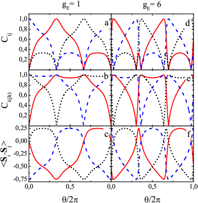
Figure 2: (color on-line) Dependence of the concurrence $C_{ij}$, $C_{i(jk)}$ and the spin correlation functions $\langle\mathbf{S}_{i}\cdot\mathbf{S}_{j}\rangle$ vs. the angle $\theta$ of the electric field calculated for the ground state. The (red) solid curves represent: $C_{12}$, $C_{1(23)}$ and $\langle\mathbf{S}_{1}\cdot\mathbf{S}_{2}\rangle$; the (blue) dashed curves: $C_{23}$, $C_{2(13)}$ and $\langle\mathbf{S}_{2}\cdot\mathbf{S}_{3}\rangle$; the (black) dotted curves: $C_{13}$, $C_{3(12)}$ and $\langle\mathbf{S}_{1}\cdot\mathbf{S}_{3}\rangle$. Left panel is plotted for a small electric field $g_{E}=1$, right one is for a large electric field $g_{E}=6$. The other parameters are: $U=20$, $\epsilon_{i}=0$ and $t$ is taken as unity.

Let us first study how entanglement can be modified by an electric field only (in the absence of the magnetic field, i.e. for $\phi=0$ and $J_{\chi}=0$). The electric field breaks the symmetry of the system, induces polarization (altought its value is small due to the strong onsite repulsion $U$). The electric field also changes the concurrence $C_{ij}$, $C_{i(jk)}$ and the spin correlation function $\langle\mathbf{S}_{i}\cdot\mathbf{S}_{j}\rangle$. Fig.2 shows these quantities for the ground state as a function of the angle $\theta$ of the electric field with respect to the axes of the system. The left panels are plotted for a small electric filed ($g_{E}=1$), when the linear Stark effect dominates. The period of oscillation is $2\pi$ for $C_{ij}$, $C_{i(jk)}$ and $\langle\mathbf{S}_{i}\cdot\mathbf{S}_{j}\rangle$. One can see in Fig.2a that for $\theta=0$ the concurrence $C_{12}=C_{13}=0$ and $C_{23}=1$. The spins in the qubit $2$ and $3$ are fully entangled which means monogamy. The spin in the qubit 1 is separated from two others (see also the red solid curve Fig.2b showing that $C_{1(23)}=0$ at $\theta=0$). The spin correlation functions (Fig.2c) $\langle\mathbf{S}_{1}\cdot\mathbf{S}_{2}\rangle=\langle\mathbf{S}_{1}\cdot\mathbf{S}_{3}\rangle=0$ and $\langle\mathbf{S}_{2}\cdot\mathbf{S}_{3}\rangle=-0.75$ which means that the spins $2$ and $3$ are in the singlet state. The wave function has the form: $|\Psi_{D_{1/2}}\rangle=|D_{1/2}\rangle_{1}$. According to the classification Sabin we have the simply biseparable states for which the density matrix can be written as $\rho=\rho_{1}\otimes\rho_{23}$. At $\theta=0$ the electric field is oriented to the quantum dot $1$ and the system has the mirror symmetry with the exchange couplings $J_{12}=J_{13}<J_{23}$ [see (18)-(20)]. A similar situation occurs for $\theta=2\pi/3$ and $4\pi/3$, only if $g_{E}<4|t|$.

For a large electric field $g_{E}>4|t|$ the situation is different and more complex (see the right panels in Fig.2). Now, the period of oscillations is changed due to the quadratic Stark effect [the second term in Eqs.(18)-(20)]. For $\theta=0$ the ground state is $|D_{1/2}\rangle_{2}$ and we do not observe monogamy. The spin in the qubit 1 is separable from two others for $\theta_{0}$ close to $2\pi/3$ and $4\pi/3$ (see $C_{1(23)}$ in Fig.2e). The condition for monogamy is the mirror symmetry of the system. Using Eqs.(18)-(20) and $J_{12}=J_{13}<J_{23}$ one can get the angle $\theta_{0}=\arccos(-2t/g_{E})$ for separability of the qubit 1. Fig.2f shows that at $\theta_{0}$ the quantum dots 2 and 3 are fully quantumly entanglement with $\langle\mathbf{S}_{2}\cdot\mathbf{S}_{3}\rangle=-3/4$ (see the dashed curve).

IV.2 Role of magnetic flux

In the presence of the magnetic flux ($\phi\neq 0$) chirality of the spin system [described by the last term in (16)] becomes relevant dassarma ; Wen ; Katsura ; Motrunich ; Bulaevskii ; trif ; Hsieh . Recently Hsieh et al. Hsieh proposed to use chirality for quantum computations. Their quantum circuits are based on qubits encoded in chirality of electron spin complexes in systems of triangular quantum dot molecules. The magnetic flux removes degeneracy between the states with different orbital momenta and leads to spin supercurrents circulating around the triangle Wen ; Katsura . We take the expectation value of the operator trif

$$C_{z}=(4/\sqrt{3})\mathbf{S}_{1}\cdot(\mathbf{S}_{2}\times\mathbf{S}_{3})$$ (29)

as a measure of chirality.Wen In the basis of the doublets (1) and using (28) one gets the expectation value

$$\langle C_{z}\rangle=\text{i}(\alpha_{1}\alpha^{*}_{2}-\alpha^{*}_{1}\alpha_{2})=-\frac{\sqrt{3}J_{\chi}}{2\Delta}$$ (30)

in the ground state. It means that chirality depends on the splitting $\Delta$ between the doublets which can be controlled by the electric field as well.

In the absence of the electric field (when all exchange couplings are equal $J_{ij}=J$) the expectation value $\langle C_{z}\rangle=\pm 1$, because the supercurrent is $\propto\sin\phi$ and circulates clockwise or anticlockwise (for $0<\phi<\pi$ or $\pi<\phi<2\pi$, respectively). For this case the spins are delocalized and the expectation values of the spin correlation functions $\langle\vec{S}_{i}\cdot\vec{S}_{j}\rangle=-1/4$. The concurrence $C_{ij}=1/3$ and $C_{i(jk)}=\sqrt{2}/3$, which describes maximal spin mixing.

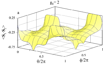
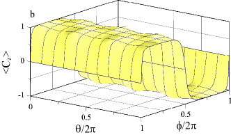
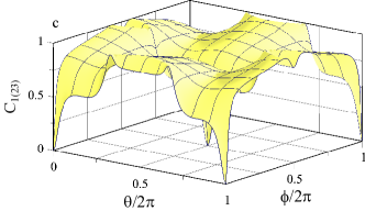
Figure 3: Plots of the spin correlation function $\langle\mathbf{S}_{1}\cdot\mathbf{S}_{2}\rangle$, the chirality $\langle C_{z}\rangle$ and the concurrence $C_{1(23)}$ in the plane $\theta$ and $\phi=2\pi\Phi/(hc/e)$ for a small electric field $g_{E}=2$ and the other parameters the same as in Fig.2.

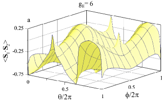
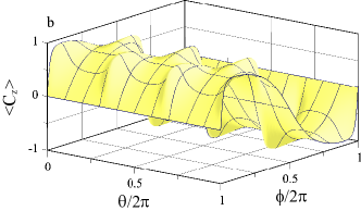
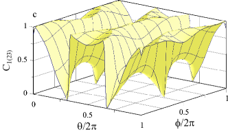
Figure 4: Plots of $\langle\mathbf{S}_{1}\cdot\mathbf{S}_{2}\rangle$, $\langle C_{z}\rangle$ and $C_{1(23)}$ in the $\theta$-$\phi$ plane for a large electric field $g_{E}=6$.

In a general situation, in the presence of both the fields, one can expect a competition between localization and delocalization of spins. These processes should manifest themselves in the spin correlation function $\langle\mathbf{S}_{i}\cdot\mathbf{S}_{j}\rangle$ (in $C_{ij}$, $C_{i(jk)}$) as well as in the expectation value of chirality $\langle C_{z}\rangle$. Fig.3 and 4 present plots for $\langle\mathbf{S}_{1}\cdot\mathbf{S}_{2}\rangle$, $\langle C_{z}\rangle$ and $C_{1(23)}$ in the $\theta$-$\phi$ plane for a small and large electric field, respectively. Close to $\phi=0$ and $\pi$ the spin supercurrent ($\propto\sin\phi$) is small and the Stark effect dominates. In the other regions the magnetic flux becomes relevant and $\langle C_{z}\rangle$ reaches its extremal value $\pm 1$ (see the plateau with small oscillations caused by the electric field in Fig.3b). According to (30) $\langle C_{z}\rangle$ is inversely proportional to the energy gap $\Delta$ between the doublet states and reaches maximal values at the symmetry points $\theta=0$, $2\pi/3$ and $4\pi/3$ (see also Fig.4b). The functions $\langle\mathbf{S}_{1}\cdot\mathbf{S}_{2}\rangle$ and $C_{1(23)}$ are very sensitive to symmetry breaking caused by the electric field. They show changes when the electric field becomes larger $g_{E}>4|t|\cos\phi$ (compare Fig.3 and 4). A detail analysis of the plots shows two contributions to the Stark effect: a linear and quadratic ones. The magnetic flux reduces the linear component, and the quadratic Stark effect dominates [see also Eqs.(18)-(20) for the exchange couplings $J_{ij}$]. If $g_{E}$ increases, the spins become more localized and the amplitude of the Stark oscillations, seen in $\langle\mathbf{S}_{1}\cdot\mathbf{S}_{2}\rangle$ and $C_{1(23)}$, increases. The localization process is monotonic, we could not observe any drastic changes - in contrast to the situation in the region close to $\phi=0$ and $\pi$ when the spin correlation functions and the concurrence change drastically their characteristics in large electric fields.

V Conclusions

Summarizing, we showed that entanglement can be controlled by the electric field in three spin system of three coherently coupled quantum dots with a triangular geometry. The studies were focussed on bipartite entanglement in the subspace of doublets with $S_{z}=+1/2$, for which the concurrence was related to the spin correlation function and the spin chirality, Eq.(13). This relation was exemplified for the Hubbard model and its canonical transformation to the effective Heisenberg model. The super-exchange coupling exhibits a linear and quadratic dependence on the electric field (the linear and quadratic spin Stark effect), which manifests itself in different periods of oscillations of the concurrence and the spin correlation functions when the electric field changes its orientation. The competition between these two Stark effects leads to different characteristics of the concurrence for a small and large electric field. For a special field orientation we found a biseparable state, for which one of the spins is separated from two others fully quantumly entangled (monogamy). For small fields one should direct the field precisely toward the quantum dot ($\theta_{0}=0$, $2\pi/3$ and $4\pi/3$) to get the spin separation at this dot. In the case of the large electric field its orientation $\theta_{0}$ should be different: the angle $\theta_{0}$ depends on the strength of the field and it should be directed toward one of the opposite quantum dots.

We also considered a role of spin chirality on entanglement. The magnetic flux $\Phi$ induces circulation of spin supercurrents and leads to spin delocalization. The bipartite concurrence becomes uniform. For small electric fields the spins are delocalized, the Stark effect can be only seen in a very narrow range of $\Phi$. For larger fields the Stark effect becomes more visible, the concurrence and the spin correlations exhibit oscillations as a function of the angle $\theta$ of the electric field. Analyzing the oscillations one can see how the magnetic flux modifies relative contributions of the linear and quadratic Stark effect to entanglement.

Our studies can be also related to recent experiments on coherent spin manipulation in three quantum dots laird10 ; takakura ; gaudreu . We showed that the scheme proposed by Di Vincenzo et al. vinzenzo , with logical qubits encoded in the doublet subspace $|D_{1/2}\rangle_{1}$ and $|D_{1/2}\rangle_{2}$, can be realized due to the spin Stark effect, in which the electric field changes spin entanglement. The ground state is a superposition of the doublet states, which can be controlled changing orientation of the electric field. Therefore, this effect can be used to preparation of a proper initial quantum state and control a logical operation. Let us point out that Di Vincenzo’s et al. scheme is different than operations between quadruplet and doublet states performed by Gaudreau et al. gaudreu in the experiment in triple quantum dots and between the singlet and triplet states in double quantum dots 2qd , where passages were accompanied by reorientation of nuclear spins in quantum dots. Within Di Vincenzo’s et al. scheme the dynamical passages are performed only between the doublet states (without nuclear spins) and total spin $S=1/2$ as well as its z-component $S_{z}=1/2$ are conserved.

- (1) R. Horodecki, P. Horodecki, M. Horodecki, K. Horodecki, Rev. Mod. Phys. 81, 865 (2009).
- (2) L. Amico, R. Fazio, A. Osterloh, V. Vedral, Rev. Mod. Phys. 80, 517 (2008).
- (3) A. Barenco, C.H. Bennett, R. Cleve, D.P. DiVincenzo, N. Margolus, P. Shor, T. Sleator, J.A. Smolin, and H. Weinfurter, Phys. Rev. A 52, 3457 (1995).
- (4) G. Burkard, D. Loss, D. P. DiVincenzo, and J. A. Smolin, Phys. Rev. B 60, 11404 (1999).
- (5) D. P. DiVincenzo, D. Bacon, J. Kempe, G. Burkard, and K. B. Whaley, Nature (London) 408, 339 (2000).
- (6) Y. S. Weinstein, and C. S. Hellberg, Phys. Rev. A 72, 022319 (2005).
- (7) C.P. Yang and J. Gea-Banacloche, Phys. Rev. A 63, 022311 (2001).
- (8) W. Dür, G. Vidal and J. I. Cirac, Phys. Rev. A 62, 062314 (2000).
- (9) Ch. F. Roos, M. Riebe, H. Häffner, W. Hänsel, J. Benhelm, G. P. T. Lancaster, Ch. Becher, F. Schmidt-Kaler, and R. Blatt, Science 304, 5676 (2004); L. DiCarlo, M. D. Reed, L. Sun, B. R. Johnson, J. M. Chow, J. M. Gambetta, L. Frunzio, S. M. Girvin, M. H. Devoret, and R. J. Schoelkopf, Nature 467, 574 (2010).
- (10) M. Neeley, R. C. Bialczak, M. Lenander, E. Lucero, M. Mariantoni, A. D. O’Connell, D. Sank, H. Wang, M. Weides, J. Wenner, Y. Yin, T. Yamamoto, A. N. Cleland, and J. Martinis, Nature 467, 570 (2010).
- (11) E. A. Laird, J. M. Taylor, D. P. DiVincenzo, C. M. Marcus, M. P. Hanson, and A. C. Gossard, Phys. Rev. B 82, 075403 (2010).
- (12) T. Takakura, M. Pioro-Ladriere, T. Obata, Y.-S. Shin, R. Brunner, K. Yoshida, T. Taniyama, and S. Tarucha, Appl. Phys. Lett. 97, 212104 (2010).
- (13) L. Gaudreau, G. Granger, A. Kam, G. C. Aers, S. A. Studenikin, P. Zawadzki, M. Pioro-Ladriere, Z. R. Wasilewski and A. S. Sachrajda, Nature Phys. 8, 54 (2012).
- (14) Y. Kato, R. C. Myers, D. C. Driscoll, A. C. Gossard, J. Levy, and D. D. Awschalom, Science 299, 1201 (2003).
- (15) V. N. Golovach, M. Borhani, and D. Loss, Phys. Rev. B 74, 165319 (2006).
- (16) E. A. Laird, C. Barthel, E. I. Rashba, C. M. Marcus, M. P. Hanson, and A. C. Gossard, Phys. Rev. Lett. 99, 246601 (2007).
- (17) M. Pioro-Ladriere, T. Obata, Y. Tokura, Y. S. Shin, T. Kubo, K. Yoshida, T. Taniyama, S. Tarucha, Nature Physics 4, 776 (2008).
- (18) J. A. Gupta, R. Knobel, N. Samarth, and D. D. Awschalom, Science 292, 2458 (2001).
- (19) A. Imamoglu, D. D. Awschalom, G. Burkard, D. P. DiVincenzo, D. Loss, M. Sherwin, and A. Small, Phys. Rev. Lett. 83, 4204 (1999).
- (20) R. Hanson, L. P. Kouwenhoven, J. R. Petta, S. Tarucha, and L. M. K. Vandersypen, Rev. Mod. Phys. 79, 1217 (2007), and references therein.
- (21) K.-Y. Choi, Z. Wang, H. Nojiri, J. van Tol, P. Kumar, P. Lemmens, B. S. Bassil, U. Kortz, and N. S. Dalal, Phys. Rev. Lett. 108, 067206 (2012).
- (22) R. Pauncz, The Construction of Spin Eigenfunctions, (Kluwer Academic/Plenum Publisher, New York, 2000).
- (23) B. Röthlisberger, J. Lehmann, D.S. Saraga, P. Traber and D. Loss, Phys Rev. Lett. 100, 100502 (2008).
- (24) X. Wang, Phys. Rev. A 64, 012313 (2001).
- (25) A. Miyake, Phys. Rev. A 67, 012108 (2003).
- (26) A. Acin, D. Bruß, M. Lewenstein, and A. Sanpera, Phys. Rev. Lett. 87, 040401 (2001).
- (27) C. Sabin and G. Garcia-Alcaine, Eur. Phys. J. D 48, 435 (2008).
- (28) V. Coffman, J. Kundu and W. K Wootters, Phys. Rev. A 61, 052306 (2000).
- (29) C. H. Bennett,, D. P. DiVincenzo, J. A. Smolin, and W. K. Wootters, Phys. Rev. A 54, 3824 (1996).
- (30) B.R. Bułka, T. Kostyrko, J. Łuczak, Phys. Rev. B 83, 035301 (2011).
- (31) T. Kostyrko and B.R. Bułka, Phys. Rev. B 84, 035123 (2011).
- (32) V. W. Scarola, and S. Das Sarma, Phys. Rev. A 71, 032340 (2005).
- (33) X. G. Wen, F. Wilczek, and A. Zee, Phys. Rev. B 39, 11413 (1989).
- (34) H. Katsura, N. Nagaosa, and A. V. Balatsky, Phys. Rev. Lett. 95, 057205 (2005).
- (35) O. I. Motrunich, Phys. Rev. B 73, 155115 (2006).
- (36) L. N. Bulaevskii, C. D. Batista, M.V.Mostovoy, and D. I.Khomskii, Phys. Rev. B 78, 024402 (2008).
- (37) M. Trif, F. Troiani, D. Stepanenko and D. Loss, Phys. Rev. Lett. 101, 217201 (2008); M. Trif, F. Troiani, D. Stepanenko and D. Loss, Phys. Rev. B 82, 045429 (2010).
- (38) C.-Y. Hsieh, and P. Hawrylak, Phys. Rev. B 82, 205311 (2010).
- (39) see for example: J. R. Petta, A. C. Johnson, J. M. Taylor, E. A. Laird, A. Yacoby, M. D. Lukin, C. M. Marcus, M. P. Hanson, and A. C. Gossard, Science 309, 2180 (2005); F. H. L. Koppens, C. Buizert, K. J. Tielrooij, I. T. Vink, K. C. Nowack, T. Meunier, L. P. Kouwenhoven, and L. M. K. Vandersypen, Nature (London) 442, 766 (2006); R. Hanson, L. P. Kouwenhoven, J. R. Petta, S. Tarucha, and L. M. K. Vandersypen, Rev. Mod. Phys. 79, 1217 (2007); M. Pioro-Ladriere, T. Obata, Y. Tokura, Y. S. Shin, T. Kubo, K. Yoshida, T. Taniyama, and S. Tarucha, Nature Phys. 4, 776 (2008).