3D Model Assisted Image Segmentation
 

Abstract

The problem of segmenting a given image into coherent regions is important in Computer Vision and many industrial applications require segmenting a known object into its components. Examples include identifying individual parts of a component for process control work in a manufacturing plant and identifying parts of a car from a photo for automatic damage detection. Unfortunately most of an object’s parts of interest in such applications share the same pixel characteristics, having similar colour and texture. This makes segmenting the object into its components a non-trivial task for conventional image segmentation algorithms. In this paper, we propose a “Model Assisted Segmentation” method to tackle this problem. A 3D model of the object is registered over the given image by optimising a novel gradient based loss function. This registration obtains the full 3D pose from an image of the object. The image can have an arbitrary view of the object and is not limited to a particular set of views. The segmentation is subsequently performed using a level-set based method, using the projected contours of the registered 3D model as initialisation curves. The method is fully automatic and requires no user interaction. Also, the system does not require any prior training. We present our results on photographs of a real car.

Keywords. Image segmentation; 3D-2D Registration; 3D Model; Monocular; Full 3D Pose; Contour Detection; Fully Automatic.

1 Introduction

Image segmentation is a fundamental problem in computer vision. Most standard image segmentation techniques rely on exploiting differences between pixel regions such as color and texture. Hence, segmenting sub-parts of an object which have similar characteristics can be a daunting task. We propose a method that performs such sub-segmentation and does not require user interaction or prior training. A result from our method is shown in Figure 1 with the car sub-segmented into a collection of parts. This includes the hood of the car, windshield, fender, front and back doors/windows.

Many industry applications require an image of a known object to be sub-segmented and separated into its parts. Examples include identification of individual parts of a car given a photograph for automatic damage identification or the identification of sub-parts of a component in a manufacturing plant for process control work. Sub-segmenting parts of an object which share the same color and texture is very hard, if not impossible, with conventional segmentation methods. However, prior knowledge of the shape of the known object and its components can be exploited to make this task easier. Based on this rationale we propose a novel Model Assisted Segmentation method for image segmentation.

We propose to register a 3D model of the known object over a given photograph/image in order to initialise the segmentation process. The segmentation is performed over each part of the object in order to obtain sub-segments from the image. A major contribution of this work is a novel gradient based loss function, which is used to estimate the full 3D pose of the object in the given image. The projected parts of the 3D model may not perfectly match the corresponding parts in the photo due to dents in a damaged vehicle or inaccuracies in the 3D model. Therefore, a level-set [11] based segmentation method is initialised using initial contour information obtained by projecting parts of the 3D model at this 3D pose. We focus our work on sub-segmentation of known car images. Cars pose a difficult segmentation task due to highly reflective surfaces in the car body. The method can be adapted to work for any object.

The remainder of this paper is organised as follows. Previous work related to our paper is described in Section 2. We describe the method used to estimate the 3D pose of the object in Section 3. The contour based image segmentation approach is described next in Section 4. This is followed by results on real photos which are benchmarked against state of the art methods in Section 5.

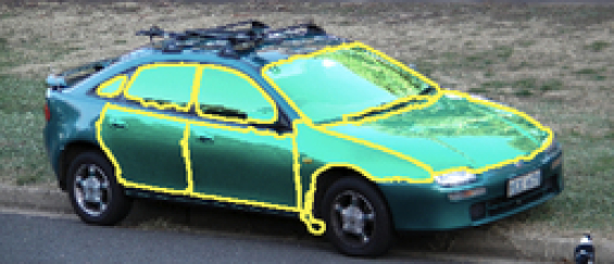
Figure 1: The figure shows ‘Model Assisted Segmentation’ results for a semi-profile view of the car.

2 Related Work

Model based object recognition has received considerable attention in computer vision. A survey by Chin and Dyer [5] shows that model based object recognition algorithms generally fall into three categories, based on the type of object representation used - namely 2D representations, 2.5D representations and 3D representations.

2D representations [18, 28] aim to identify the presence and orientation of a specific face of 3D objects, for example parts on a conveyor belt. These approaches require prior training to determine which face to match to, and are unable to generalise to other faces of the same object.

2.5D approaches [19, 8, 7] are also viewer centred, where the object is known to occur in a particular view. They differ from the 2D approach as the model stores additional information such as intrinsic image parameters and surface-orientation maps.

3D approaches are utilised in situations where the object of interest can appear in a scene from multiple viewing angles. Common 3D representation approaches can be either an ‘exact representation’ or a ‘multi-view feature representation’. The latter method uses a composite model consisting of 2D/2.5D models for a limited set of views. Multi-view feature representation is used along with the concept of generalised cylinders by Brooks and Binford [3] to detect different types of industrial motors in the so called ACRONYM system. The models used in the exact representation method, on the contrary, contain an exact representation of the complete 3D object. Hence a 2D projection of the object can be created for any desired view. Unfortunately, this method is often considered too costly in terms of processing time. The 2D and 2.5D representations are insufficient for general purpose applications. For example, a vehicle may be photographed from an arbitrary view in order to indicate the damaged parts. Similarly, the 3D multi-view feature representation is also not suitable, as we are not able to limit the pose of the vehicle to a small finite set of views. Therefore, pose identification has to be done using an exact 3D model. Little work has been done to date on identifying the pose of an exact 3D model from a single 2D image.

Image gradients. Gray scale image gradients have been used to estimate the 3D pose in traffic video footage from a stationary camera by Kollnig and Nagel [10]. The method compares image gradients instead of simple edge segments, for better performance. Image gradients from projected polyhedral models are compared against image gradients in video images. The pose is formulated using three degrees of freedom; two for position and one for angular orientation. Tan and Baker [27] use image gradients and a Hough transform based algorithm for estimating vehicle pose in traffic scenes, once more describing the pose via three degrees of freedom. Pose estimation using three degrees of freedom is adequate for traffic image sequences, where the camera position remains fixed with respect to the ground plane. This approach does not recover the full 3D pose as in our method.

Feature-based methods [6, 15] attempt to simultaneously solve the pose and point correspondence problems. The success of these methods are affected by the quality of the features extracted from the object, which is non-trivial with objects like cars. Features depend on the object geometry and can cause problems when recovering a full 3D pose. Also different image modalities cause problems with feature based methods. For example reflections which may appear as image features do not occur in the 3D model projection. Our method on the contrary, does not depend on feature extraction.

Segmentation. The use of shape priors for segmentation and pose estimation have been investigated in [22, 21, 23, 25]. These methods focus on segmenting foreground from background using 3D free-form contours. Our method, on the contrary, does intra-object segmentation (into sub-segments) by initialising the segmentation using projections of 3D CAD model parts at an estimated pose. In addition, our method works on more complex objects like real cars.

3 3D Model Registration

We describe the use of a featureless gradient based loss function which is used to register the 3D model over the 2D photo. Our method works on triangulated 3D CAD models with a large number of polygons (including 3D models obtained from laser scans) and utilises image gradients of the 3D model surface normals rather than considering simple edge segments.

Gradient based loss function. We define a gradient based loss function that has a minimum at the correct 3D pose $\boldsymbol{\theta}_{0}\in I\mskip-3.0mu\mskip-3.0muR^{7}$ where the projected 3D model matches the object in the given photo/image. The image gradients of the 3D model surface normal components and the image gradients of the 2D photo are used to define a loss function at a given pose $\boldsymbol{\theta}$.

We use $(u,v)\in Z\mskip-3.0mu\mskip-3.0mu\mskip-3.0muZ^{2}$ to denote 2D pixel coordinates in the photo/image and $(x,y,z)\in I\mskip-3.0mu\mskip-3.0muR^{3}$ to denote 3D coordinates of the 3D model. Let $\boldsymbol{W}$ be a $d$ dimensional matrix (for example $d=3$ if $\boldsymbol{W}$ is an RGB image) with elements $W(u,v)\in I\mskip-3.0mu\mskip-3.0muR^{d}$. We define the $k$ norm ‘gradient magnitude’ matrix of $\boldsymbol{W}$ as

$$\begin{array}[]{l}||\nabla{W(u,v)}||_{k}^{k}:=\sum_{i=1}^{d}\left(|\frac{\partial{W_{i}(u,v)}}{\partial{u}}|^{k}+|\frac{\partial{W_{i}(u,v)}}{\partial{v}}|^{k}\right)\end{array}$$ (1)

Based on this we have the gradient magnitude matrix $\boldsymbol{G_{I}}$ for a 2D photo/image $\boldsymbol{I}$ as

$$\begin{array}[]{l}{G_{I}}(u,v)=||\nabla{I(u,v)}||_{k}^{k}\end{array}$$ (2)

Let $\boldsymbol{\phi}(x,y,z,\boldsymbol{\theta})=\left(\phi_{x}\mskip 5.0mu plus 5.0mu\phi_{y}\mskip 5.0mu plus 5.0mu\phi_{z}\right)^{T}\in I\mskip-3.0mu\mskip-3.0muR^{3}$ be the unit surface normal at the 3D point $p=(x,y,z)$ for the 3D model at pose $\boldsymbol{\theta}$. The model is rendered with the surface normal components values $\phi_{x}$, $\phi_{y}$ and $\phi_{z}$ used as RGB color values in the OpenGL renderer to obtain the projected surface normal component matrix $\boldsymbol{\Phi}$ such that $\Phi(u,v,\boldsymbol{\theta})\in I\mskip-3.0mu\mskip-3.0muR^{3}$ has surface normal component values at the 2D point $(u,v)$ in the projected image. Based on this we have the gradient normal matrix for the surface normal components as

$$\begin{array}[]{l}{G_{N}(\boldsymbol{\theta})(u,v)}=||\nabla{\Phi(u,v,\boldsymbol{\theta})}||_{k}^{k}\end{array}$$ (3)

The loss function $L_{g}(\boldsymbol{\theta})$ for a given pose $\boldsymbol{\theta}$ is defined as

$$\begin{array}[]{l}L_{g}(\boldsymbol{\theta}):=1-(corr(\boldsymbol{G_{N}(\boldsymbol{\theta})},\boldsymbol{G_{I}}))^{2}\in[0,1]\end{array}$$ (4)

where $corr(\boldsymbol{G_{N}(\boldsymbol{\theta})},\boldsymbol{G_{I}})$ is the Pearson’s product-moment correlation coefficient [20] between the matrix elements of $\boldsymbol{G_{N}(\boldsymbol{\theta})}$ and $\boldsymbol{G_{I}}$. This loss has a convenient property of ranging between $0$ and $1$. Lower loss values imply a better 3D pose.

Visualisation. We illustrate intermediate steps of the loss calculation for a 3D model of a Mazda 3 car. The surface normal components $\Phi_{x}(u,v,\boldsymbol{\theta})$ $\Phi_{y}(u,v,\boldsymbol{\theta})$ and $\Phi_{z}(u,v,\boldsymbol{\theta})$ are shown in Figure 2(a-c). Their image gradients are shown in Figure 2(d-i) and the resulting $\boldsymbol{G_{N}(\boldsymbol{\theta})}$ matrix image is shown in Figure 2(j). Similarly intermediate steps in the calculation of $\boldsymbol{G_{I}}$ are show in Figure 3 for a real photo and a synthetic photo. We show overlaid images of $\boldsymbol{G_{N}(\boldsymbol{\theta})}$ and $\boldsymbol{G_{I}}$ at the known matching pose $\boldsymbol{\theta}$ in Figure 4. We show how the overlap changes by applying $2$ levels of Gaussian smoothing (described below) in Figures 4 for the real and synthetic photo. The synthetic photos were made by projecting the 3D model at a known pose $\boldsymbol{\theta}$.

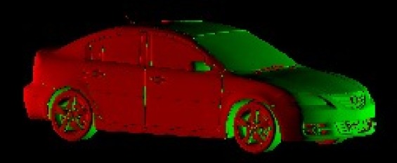
(a) $\Phi_{x}(u,v,\boldsymbol{\theta})$

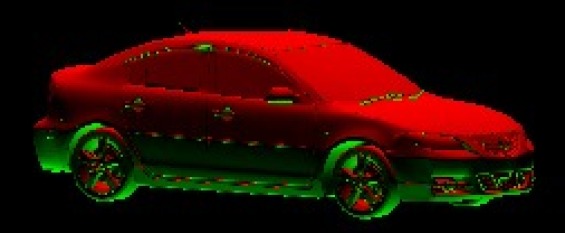
(b) $\Phi_{y}(u,v,\boldsymbol{\theta})$

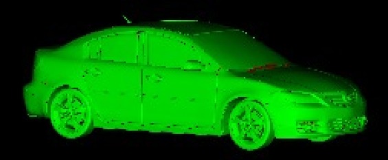
(c) $\Phi_{z}(u,v,\boldsymbol{\theta})$

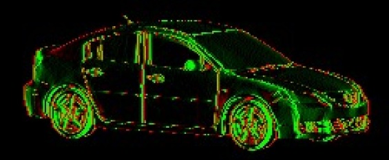
(d) $\frac{\partial\Phi_{x}(u,v,\boldsymbol{\theta})}{\partial{u}}$

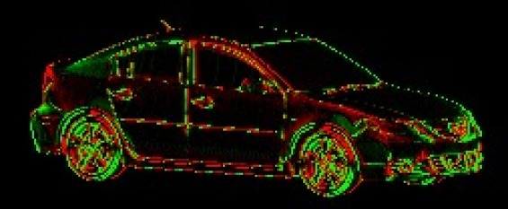
(e) $\frac{\partial\Phi_{x}(u,v,\boldsymbol{\theta})}{\partial{v}}$

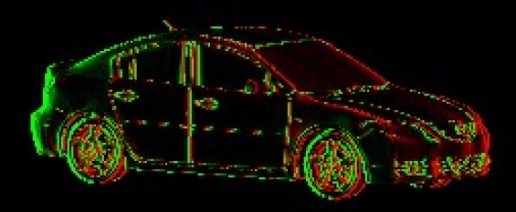
(f) $\frac{\partial\Phi_{y}(u,v,\boldsymbol{\theta})}{\partial{u}}$

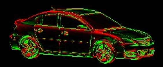
(g) $\frac{\partial\Phi_{y}(u,v,\boldsymbol{\theta})}{\partial{v}}$

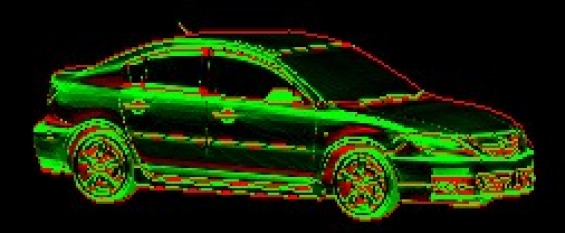
(h) $\frac{\partial\Phi_{z}(u,v,\boldsymbol{\theta})}{\partial{u}}$

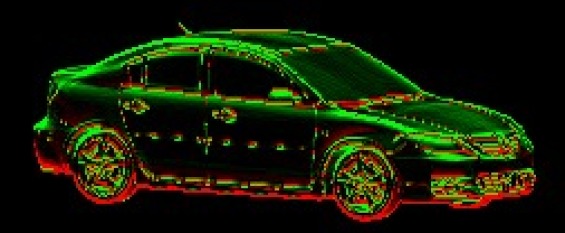
(i) $\frac{\partial\Phi_{z}(u,v,\boldsymbol{\theta})}{\partial{v}}$

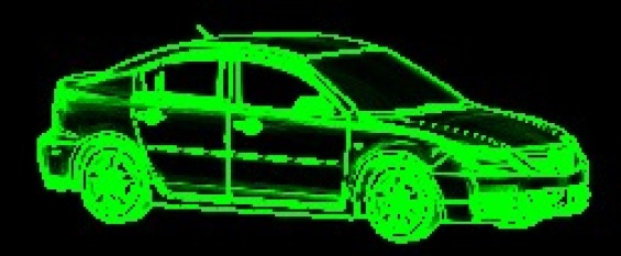
(j) $\boldsymbol{G_{N}(\boldsymbol{\theta})}$

Figure 2: The visualisations shows $\boldsymbol{G_{N}(\boldsymbol{\theta})}$ for a 3D model in 2(j). The x,y and z component matrices of the surface normal vector are shown in 2(a)-2(c). Their image gradients are shown in 2(d)-2(i). The resulting $\boldsymbol{G_{N}(\boldsymbol{\theta})}$ matrix is shown in 2(j). No Gaussian smoothing has been applied. Colour representation: green=positive, black=zero and red=negative. We use a horizontal $x$ axis pointing left to right, vertical $y$ axis and pointing top to bottom and an $z$ axis which points out of the page.

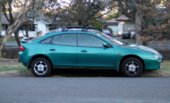
(a) Real photo

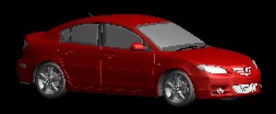
(b) Synthetic photo

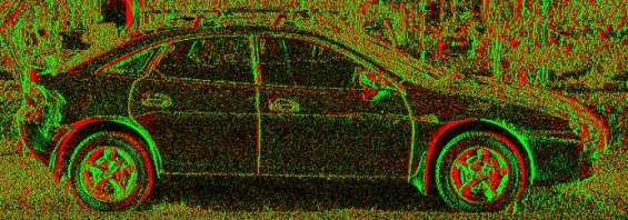
(c) Real $\frac{\partial\boldsymbol{I}}{\partial{u}}$

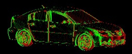
(d) Synthetic $\frac{\partial\boldsymbol{I}}{\partial{u}}$

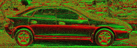
(e) Real $\frac{\partial\boldsymbol{I}}{\partial{v}}$

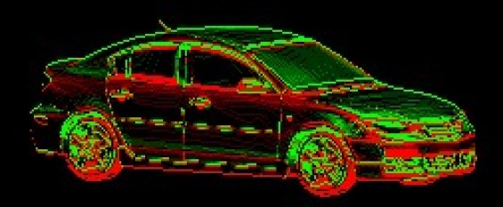
(f) Synthetic $\frac{\partial\boldsymbol{I}}{\partial{v}}$)

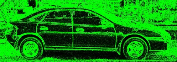
(g) Real $\boldsymbol{G_{I}}$

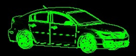
(h) Synthetic $\boldsymbol{G_{I}}$

Figure 3: Intermediate steps in calculating $\boldsymbol{G_{I}}$ for a real (column 1) and synthetic photo (column 2). The synthetic photo was made by projecting the 3D model. Image gradients (rows 2 and 3) and $\boldsymbol{G_{I}}$ (row 4) are shown. Colour representation: green=positive, black=zero and red=negative.

(a) Real

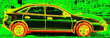
(b) n=0

(c) n=2

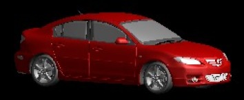
(d) Synthetic

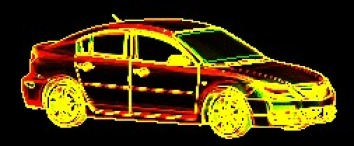
(e) n=0

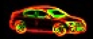
(f) n=2

Figure 4: Overlaid images of $\boldsymbol{G_{I}}$ and $\boldsymbol{G_{N}(\boldsymbol{\theta})}$ for a real photo (row 1) and a synthetic photo (row 2) obtained by rendering a 3D model are shown. The first column shows the photos $\boldsymbol{I}$. The overlaid images of $\boldsymbol{G_{I}}$ and $\boldsymbol{G_{N}(\boldsymbol{\theta})}$ with no Gaussian smoothing (column 2) and 3 levels of Gaussian smoothing (column 3) are shown. The photo is in the green channel and 3D model is in the red channel, with yellow showing overlapping regions.

The correlation will be highest in Equation 4 when the 3D model is projected with pose parameters $\boldsymbol{\theta}_{0}$ that match the object in the photo $F$, as this has the best overlap. Therefore the loss will be lowest at the correct pose parameters $\boldsymbol{\theta}_{0}$, for values of $\boldsymbol{\theta}$ reasonably close to $\boldsymbol{\theta}_{0}$. We see this in the loss landscapes in Figure 6.

Gaussian smoothing. We do Gaussian smoothing on the photo and rendered surface normal component images before calculating $\boldsymbol{G_{I}}$ (Equation 2) and $\boldsymbol{G_{N}(\boldsymbol{\theta})}$ (Equation 3). This is done by convolving with a 2D Gaussian kernel followed by down-sampling [7]. This makes the loss function landscape less steep and noisy, thus making it easier to optimise. However, the global optimum tends to deviate slightly from the correct pose at high levels of Gaussian smoothing. Compare the 1D loss landscapes shown in Figure 6 for different levels of Gaussian smoothing $n$. Therefore, we do a series of optimisations starting from the highest level of smoothing, using the optimum found at level $n$ as the initialisation for level $n-1$, recursively.

Choosing the norm $k$. We have a choice when selecting the norm for Equations 2 and 3. Having tested both $1$-norm and $2$-norm cases we have found the $1$-norm to be less noisy (as shown in Figure 6) and hence easier to optimise.

Initialisation. We use a rough pose estimate to seed the optimisation. An object specific method can be used to obtain the rough pose. Possible methods for obtaining a coarse initial pose include the work done by [17], [26] and [1]. We have used the wheel match method developed by Hutter and Brewer [9] to obtain an initial pose for vehicle photos where the wheels are visible. The wheels need not be visible with the other methods mentioned above. We use the following to represent the rough pose of cars as prescribed in [9] which neglects the effects of perspective projection.

$$\boldsymbol{\theta}^{\prime}:=\left(\mu_{x},\mu_{y},\delta_{x},\delta_{y},\psi_{x},\psi_{y}\right)$$ (5)

$\boldsymbol{\mu}=(\mu_{x},\mu_{y})$ is the visible rear wheel center of the car in the 2D image. $\boldsymbol{\delta}=(\delta_{x},\delta_{y})$ is the vector between corresponding rear and front wheel centres of the car in the 2D image. The 2D image is a projection of the 3D model on to the XY plane. $\boldsymbol{\psi}=\left(\psi_{x},\psi_{y},\psi_{z}\right)$ is a unit vector in the direction of the rear wheel axle of the 3D car model. Therefore, $\psi_{z}=-\sqrt{1-\smash{\psi_{x}^{2}-\psi_{y}^{2}}}$ and need not be explicitly included in the pose representation $\boldsymbol{\theta}$. This representation is illustrated in Figure 5.

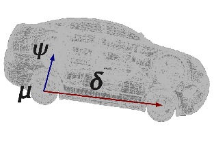
Figure 5: We illustrate components of the pose representation $\boldsymbol{\theta}^{\prime}$ (Equation 5) used for 3D models of cars. We use the rear wheel center $\boldsymbol{\mu}$, the vector between the wheel centres $\boldsymbol{\delta}$ and unit vector $\boldsymbol{\psi}$ in the direction of the rear wheel axle.

We include an additional perspective parameter $f$ (the distance to the camera from the projection plane in the OpenGL 3D frustum) when optimising the loss function to obtain the fine 3D pose. Hence we define the full 3D pose as follows.

$$\boldsymbol{\theta}:=\left(\mu_{x},\mu_{y},\delta_{x},\delta_{y},\psi_{x},\psi_{y},f\right)$$ (6)

$\boldsymbol{\theta}^{\prime}$ is converted to translation, scale and rotation as per [9] to transform the 3D model and along with $f$ is used to render the 3D model with perspective projection in OpenGL using pose $\boldsymbol{\theta}$. Thereby, we estimate the full 3D pose by minimizing Equation 4 w.r.t $\boldsymbol{\theta}$. Intrinsic camera parameters need not be known explicitly. Note that any other choice of pose parameters would do. We use the above as it is convenient with cars.

Background removal. As the effects of the background clutter in the photo adds considerable noise to the loss function landscape we use an adaptation of the Grabcut [24] method to remove a considerable amount of the background pixels from the photo. Although, this does not result in a perfect removal of the background it significantly improves the pose estimation results. The initial rough pose estimate is used as a prior to generate the background and foreground grabcut masks . Figure 7(b) shows results of the background removal.

Optimisation. We use the downhill simplex optimiser [16] to find the pose parameters $\boldsymbol{\theta}_{0}$ which give the lowest loss value for Equation 4. This optimiser is very robust and is capable of moving out of local optima by reinitialising the simplex. Downhill simplex does not require gradient calculations. Gradient based optimisers would be problematic given the loss landscapes in Figure 6. We use the fine pose obtained thus to register the 3D model on the 2D photo. This is used to initialise contour detection based image segmentation.

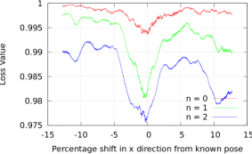
(a) 2-norm

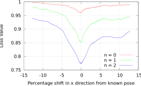
(b) 1-norm

Figure 6: We compare $1$-norm and $2$-norm loss landscapes obtained by shifting the 3D model along the x direction from a known 3D pose. The horizontal axis shows the percentage deviation along the x axis. The numbers in the legend show the level of Gaussian smoothing $n$ applied on the gradient images before calculating the loss in Equation 4. We note that the $1$-norm loss is less noisy compared to the $2$-norm loss. The actual loss function is seven dimensional and graphs of the other dimensions are similar.

4 Contour Detection

In this section, we discuss the procedure of contour detection used to segment the known object in the image. We use a variation of the level set method which does not require re-initialisation [11] to find boundaries of relevant object parts.

Most active contour models implement an edge-function to find boundaries. The edge-function is a gradient dependant positive decreasing function. A common formulation is as follows

$$g(|\nabla\boldsymbol{I}|)=\frac{1}{1+|\nabla{G_{\sigma}}\otimes\boldsymbol{I}|^{p}},\quad p\geq 1,$$ (7)

where $\boldsymbol{G_{\sigma}}\otimes\boldsymbol{I}$ denotes a smoother version of 2D image $\boldsymbol{I}$, $\boldsymbol{G_{\sigma}}$ is an isotropic Gaussian kernel with standard deviation $\sigma$, and $\otimes$ is the convolution operator. Therefore $g(|\nabla\boldsymbol{I}|)$ will be $0$, as $\nabla\boldsymbol{I}$ approaches infinity, i.e.

$$\lim_{|\nabla\boldsymbol{I}|\to\infty}g(|\nabla\boldsymbol{I}|)=0,\mskip 5.0mu plus 5.0mu\mathrm{when}\mskip 3.0mu\sigma=0.$$ (8)

As per [11], a Lipschitz function $\phi$ is used to represent the curve $C=\{(u,\mskip 5.0mu plus 5.0muv)|\phi_{0}(u,\mskip 5.0mu plus 5.0muv)=0\}$ such that ,

$$\phi_{0}(u,\mskip 5.0mu plus 5.0muv)=\left\{\begin{array}[]{ll}-\rho,&\quad(u,\mskip 5.0mu plus 5.0muv)\mskip 5.0mu plus 5.0mu\mathrm{inside\mskip 5.0mu plus 5.0mu\mskip 3.0mucontour}\mskip 5.0mu plus 5.0mu\mskip 3.0muC\\ \quad\mskip-3.0mu0,&\quad(u,\mskip 5.0mu plus 5.0muv)\mskip 5.0mu plus 5.0mu\mathrm{on\mskip 5.0mu plus 5.0mu\mskip 3.0mucontour}\mskip 5.0mu plus 5.0mu\mskip 3.0muC\\ \quad\mskip-3.0mu\rho,&\quad(u,\mskip 5.0mu plus 5.0muv)\mskip 5.0mu plus 5.0mu\mathrm{outside\mskip 5.0mu plus 5.0mu\mskip 3.0mucontour}\mskip 5.0mu plus 5.0mu\mskip 3.0muC\end{array}\right.$$ (9)

As with other level set formulations like [4] and [13], the curve $C$ is evolved using the mean curvature $\mathrm{div}\left(\nabla\phi/|\nabla\phi|\right)$ in the normal direction $|\nabla\phi|$. Therefore the curve evolution is represented by $\partial\phi/\partial t$ as

$$\begin{array}[]{ll}\frac{\partial\phi}{\partial t}=|\nabla\phi|\left(\mathrm{div}\left(g(|\nabla\boldsymbol{I}|)\frac{\nabla\phi}{|\nabla\phi|}\right)+\nu g(|\nabla\boldsymbol{I}|)\right),\\ \phi(0,\mskip 5.0mu plus 5.0muu,\mskip 5.0mu plus 5.0muv)=\phi_{0}(u,\mskip 5.0mu plus 5.0muv)\in[0,\mskip 5.0mu plus 5.0mu\infty)\times\mathbb{R}^{2}\par\end{array}$$ (10)

where the evolution of the curve is given by the zero-level curve at time $t$ of the function $\phi(t,\mskip 5.0mu plus 5.0mux,\mskip 5.0mu plus 5.0muy)$. $\nu$ is a constant to ensure that the curve evolves in the normal direction, even if the mean curvature is zero.

Theoretically, as the image gradient on an edge/boundary of an image segment tends to infinity, the edge function $g$ (Equation 7) is zero on the boundary. This causes the curve $C$ to stop evolving at the boundary (Equation 10). However, in practice the edge function may not always be zero at image boundaries of complex images and the performance of the level set method is severely affected by noise. Isotropic Gaussian smoothing can be applied to reduce image noise but over smoothing will also smooth the edges, in which case, the level set curve may miss the boundary altogether. This is a common problem not only for the level set method in [11] but also for other active contour models [4, 14, 12, 13]. Additionally, the efficiency and effectiveness of level set in boundary detection depends a lot on the initialisation of the curve. Without appropriate initialisation, the curve is frequently trapped into local minima.

A very close initialisation curve can eliminate this problem. In our approach, the initialisation curve is obtained by registering a 3D model over the photo as described in Section 3. Since the parts $p$ in the 3D model are already known, they can be projected at the known 3D pose $\boldsymbol{\theta}$ to obtain a selected part outline $o_{p}$ in 2D. An ‘erosion’ morphological operator is applied on $o_{p}$ to obtain the initial curve $\phi_{0,p}$ which is inside the real boundary.

The green curves (initialisation images in Figures 9, 10 and 11) are used to denote the 2D outlines of projected parts in the 3D model, while the red curves are the initialisation curves obtained by eroding these green curves. The level set starts with the initial curve $\phi_{0,p}$ to find actual boundary $\phi_{r,p}$ in the 2D image of vehicle, for each part $p$. The yellow curves (result images in Figures 9, 10 and 11) indicate the actual boundaries detected.

The entire process of ‘Model Assisted Segmentation’ is given in pseudo-code in Algorithm 1.

Algorithm 1 Model Assisted Segmentation

0:  Let $\boldsymbol{I}=$ Given image, $\boldsymbol{M}=$ Known 3D model

0:  Segmentation curves $\phi_{r,p}$ for selected model parts $p$

1:  $\boldsymbol{\theta}^{\prime}\leftarrow$ Rough pose from $\boldsymbol{I}$

2:  $\boldsymbol{I}^{\prime}\leftarrow$ Remove background in $\boldsymbol{I}$ using $\boldsymbol{\theta}^{\prime}$

3:  $\boldsymbol{\theta}\leftarrow\boldsymbol{\theta}^{\prime}$

4:  for $n=2$ down to 0 do

5:     $\boldsymbol{\theta}\leftarrow$ Optimise $L_{g}(\boldsymbol{\theta})$ on $\boldsymbol{I}^{\prime}$ starting from $\boldsymbol{\theta}$ using $n$ levels of Gaussian smoothing

6:  end for

7:  for $p\in$ Selected parts in $\boldsymbol{M}$ do

8:     $o_{p}\leftarrow$ Outline of $p$ projected using $\boldsymbol{\theta}$

9:     $\phi_{0,p}\leftarrow$ Apply erosion operation on $o_{p}$

10:     $\phi_{r,p}\leftarrow$ Output of level set on $\boldsymbol{I}$ using $\phi_{0,p}$ as initial curve

11:  end for

5 Results

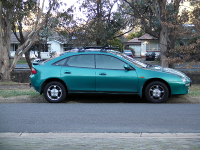
(a) Photo

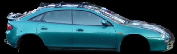
(b) Background removed

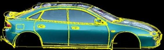
(c) Rough pose

(d) Fine pose n=2

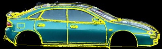
(e) Fine pose n=1

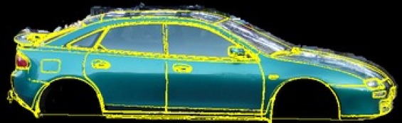
(f) Final fine pose n=0

Figure 7: The images show pose estimation results for a real photograph of a Mazda Astina car. The original photograph and subsequent images have been cropped for clarity. The fine 3D pose in 7(f) is obtained by optimising the novel gradient based loss function (Equation 4) using the rough pose in 7(c). The rough pose is obtained as prescribed in [9]. Much of the background is removed 7(b) from the original photo 7(a) using an adaptation of ‘Grabcut’ [24] when estimating the fine 3D pose. Intermediate steps of optimising the loss function with different levels of Gaussian smoothing $n$ applied on the gradient images are shown in 7(d), 7(e) and 7(f). The close ups highlight the visual improvement during intermediate steps Figure 8.

(a) n=2

(b) n=1

(c) n=0

Figure 8: Close ups at each step of the optimisation (shown in Figure 7) for different levels of Gaussian smoothing $n$ highlight the visual improvement in the 3D pose.

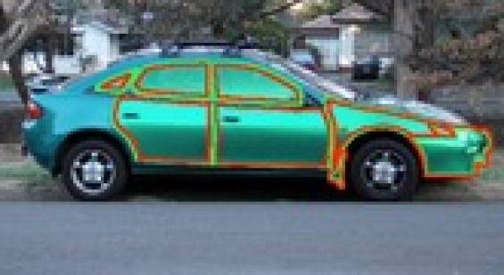
(a) Initialisation

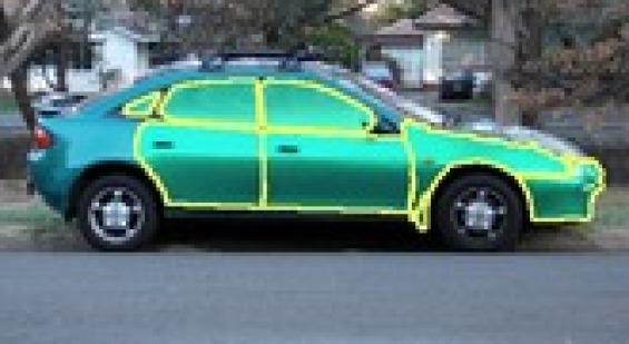
(b) Result

Figure 9: The figure shows the ‘Model Assisted Segmentation’ results for a real photo of a Mazda Astina car. The initialisation curves for a selection of car body parts are shown in 9(a) based on the fine 3D pose shown in Figure 7(f). The 3D model outlines are shown in ‘green’ and the initialisation curves obtained by eroding these outlines are shown in ‘red’. The resulting segmentation is shown in 9(b). Close ups are shown along with benchmark results in Figure 10.

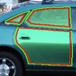
(a) Initialisation

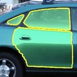
(b) Result

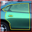
(c) Benchmark - GC

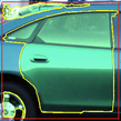
(d) Benchmark - LS

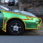
(e) Initialisation

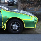
(f) Result

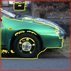
(g) Benchmark - GC

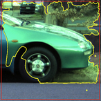
(h) Benchmark - LS

Figure 10: Different close ups (row wise) for the results in Figure 9 are shown with the initialisation curves (column 1), our results (column 2) and benchmark results (columns 3 and 4). Our results are more accurate in general. Note the bleeding and false positives in the benchmark results. Our method is more accurate and sub-segments the image into meaningful parts.

(a) Initialisation

(b) Result

(c) Benchmark - LS

(d) Benchmark - GC

(e) Initialisation

(f) Result

(g) Benchmark - GC

(h) Benchmark - LS

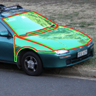
(i) Initialisation

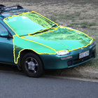
(j) Result

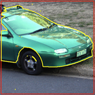
(k) Benchmark - GC

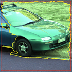
(l) Benchmark - LS

Figure 11: The figures show different close ups (row wise) for the results in Figure 1. Initialisation curves (column 1), our results (column 2) and benchmark results (columns 3 and 4) are shown. We note that our results more accurate and has sub-segmented the car into meaningful components.

We apply our method to segment components of a real car from a photograph as follows.

Pose estimation. The results of registering the 3D model over the photograph (pose estimation) are shown in Figure 7. A gradient sketch of the 3D model is drawn over the photograph in yellow to indicate the pose of the 3D model at each step in Figure 7. The wheels of the 3D model do not match the wheels in the photo due to the effects of wheel suspension. Since we are interested in segmenting parts of the car body the wheels have been removed from the 3D model for the fine pose estimation. The original photograph in Figure 7(a) shows the side view of a Mazda Astina car. We register a triangulated 3D model of the car obtained by a 3D laser scan. The rough 3D pose obtained using the wheel locations [9] is shown in Figure 7(c). The result of the approximate background removal is shown in Figure 7(b). We optimise the gradient based loss function (Equation 4) for the image in Figure 7(b) with respect to the seven pose parameters (Section 3) to obtain the fine 3D pose. The optimisation is done sequentially moving from the highest level of Gaussian smoothing to the lowest. We start from the rough pose with two levels of Gaussian smoothing and obtain the pose in Figure 7(d). Next we use this pose to initialise an optimisation of the loss function with one level of Gaussian smoothing and obtain the pose in 7(e). Finally, we use this pose to perform one more optimisation with no Gaussian smoothing and obtain the final fine 3D pose shown in Figure 7(f). We note that the visual improvement in the image overlays gets smaller as we go up the Gaussian pyramid. However, the improvement in the 3D pose becomes more apparent when we compare the close ups in Figures 8(a), 8(b) and 8(c).

Segmentation. Segmentation results based on contour detection for the photograph in 7(a) using the fine 3D pose (Figure 7(f)) are shown in Figures 9 and 10. The segmentation results for a selection of car parts (front and back doors, front and back windows, fender, mud guard and front buffer) are shown in Figure 9(b) by the yellow curves. The part boundaries obtained by projecting the 3D model are shown in green and the initialisation curves are shown in red in Figure 9(a). For the sake of clarity we also include close ups of a few parts. The initialisation curves and the segmentation results for the back door and window are shown in Figures 10(a) and 10(b), using the same color code. Close ups for the front parts are shown in Figures 10(e) and 10(f). We see the high amount of reflection in the car body deteriorating the performance of the segmentation results in the latter case, especially around the hood of the car and windshield. In contrast the mud guard, lower parts of the buffer and fender are segmented out quite well in Figure 10(f) as there is less reflection noise in that region. Results for a semi-profile view of the car are shown in Figures 1 and 11 using same convention.

Accuracy. The accuracy of the results have been compared against a ground truth obtained from the photos by hand annotation in Table 1. We calculate the accuracy as

$$\begin{array}[]{l}a=1-\frac{\sum_{u,\mskip 5.0mu plus 5.0muv}|U_{R}(u,\mskip 5.0mu plus 5.0muv)-U_{G}(u,\mskip 5.0mu plus 5.0muv)|}{\sum_{u,\mskip 5.0mu plus 5.0muv}U_{G}(u,\mskip 5.0mu plus 5.0muv)}\end{array}$$ (11)

where $U_{R}$ and $U_{G}$ are two binary images of the sub-segmentation result and ground truth respectively. We note that the accuracy is considerably high. Also, the side view has a higher accuracy in general because the pose estimation gave a better result and hence the segmentation was better initialised.

Part	Side View	Semi Profile	Avg.
Fender	97.7%	97.6%	97.7%
Front door	98.1%	95.3%	96.7%
Back door	96.8%	93.6%	95.2%
Mud flap	97.3%	95.1%	96.2%
Front window	97.8%	97.5%	97.7%
Back window	99.5%	93.9%	96.7%

Table 1: Accuracy of the sub-segmented parts measured against hand annotated ground truth.

Benchmark tests. Our results from Model Assisted Segmentation were compared with state of the art image segmentation methods ‘Grabcut (GC)’ [24] and ‘Level set (LS)’ [11] which do not use any Model Assistance. A bounding box has been used initialise the benchmark methods. We compare our results (Figures 10(b) and 10(f)) with the benchmark tests in Figure 10. The segmentation using our method are more accurate in general. In addition to this, our method has the added advantage of sub-segmenting parts of the same object. This is a non-trivial task for conventional segmentation methods when the sub-segments of the object share the same colour and texture. In terms of overall performance, we observe that in our method the segmentation results ‘bleed’ a lot less into adjacent areas, unlike with the benchmark results. In terms of sub-segmenting parts of the same object, we see in Figure 10(f) that our method is capable of successfully segmenting out the fender, mud guard and the buffer from the front door unlike the benchmark methods. In fact it would be extremely difficult (if not impossible) to sub-segment parts of the front of the car which are painted the same color with conventional methods. Similarly the back door, back window and the smaller glass panel have been segmented out in Figure 10(b) where as the benchmark methods group them together. Results for a semi-profile view of the car are shown in Figure 1 with close ups and benchmark comparisons in Figure 11. Our results are better and separate the object into meaningful parts.

6 Discussion

The Model Assisted Segmentation method described in this paper can segment parts of a known 3D object from a given image. It performs better than the state of the art and can segment (and separate) parts that have similar pixel characteristics. We present our results on images of cars. The highly reflective surfaces of cars make the pose estimation as well as the segmentation tasks more difficult than with non-reflective objects.

We note that a close initialisation curve obtained from the 3D pose estimation significantly improves the performance of contour detection, and hence the image segmentation. However, the presence of reflections can deteriorate the quality of the results. We intend to explore avenues to make the process more robust in the presence of reflections.

Acknowledgment. The authors wish to thank Stephen Gould and Hongdong Li for the valuable feedback and advice. This work was supported by Control C=xpert.

References

- [1] M. Arie-Nachimson and R. Basri. Constructing implicit 3d shape models for pose estimation. In ICCV, 2009.
- [2] G. Bradski. The OpenCV Library. Dr. Dobb’s Journal of Software Tools, 2000.
- [3] Brooks, R. A., and Binford, T. O. Geometric modelling in vision for manufacturing. In Proceedings of the Society of Photo-Optical Instrumentation Engineers Conference on Robot Vision, volume 281, pages 141–159, Washington, DC, USA, April 1981.
- [4] V. Caselles, F. Catté, T. Coll, and F. Dibos. A geometric model for active contours in image processing. Numerische Mathematik, 66(1):1–31, 1993.
- [5] Roland T. Chin and Charles R. Dyer. Model-based recognition in robot vision. ACM Comput. Surv., 18(1):67–108, 1986.
- [6] P. David, D. DeMenthon, R. Duraiswami, and H. Samet. SoftPOSIT: Simultaneous pose and correspondence determination. International Journal of Computer Vision, 59(3):259–284, 2004.
- [7] David A. Forsyth and Jean Ponce. Computer Vision: A Modern Approach. Prentice Hall Professional Technical Reference, 2002.
- [8] B.K.P. Horn. Obtaining shape from shading information. In PsychCV75, pages 115–155, 1975.
- [9] M. Hutter and N. Brewer. Matching 2-D Ellipses to 3-D Circles with Application to Vehicle Pose Identification. In Image and Vision Computing New Zealand, 2009. IVCNZ’09. 24th International Conference, pages 153–158, 2009.
- [10] Henner Kollnig and Hans-Hellmut Nagel. 3d pose estimation by directly matching polyhedral models to gray value gradients. Int. J. Comput. Vision, 23(3):283–302, 1997.
- [11] Chunming Li, Chenyang Xu, Changfeng Gui, and M.D. Fox. Level set evolution without re-initialization: a new variational formulation. In Computer Vision and Pattern Recognition, 2005. CVPR 2005. IEEE Computer Society Conference on, volume 1, pages 430 – 436 vol. 1, june 2005.
- [12] R. Malladi, J. Sethian, and B. Vemuri. Evolutionary fronts for topology-independent shape modeling and recovery. Computer Vision—ECCV’94, pages 1–13, 1994.
- [13] R. Malladi, J.A. Sethian, and B.C. Vemuri. Shape modeling with front propagation: A level set approach. Pattern Analysis and Machine Intelligence, IEEE Transactions on, 17(2):158–175, 2002.
- [14] Ravikanth Malladi. A topology-independent shape modeling scheme. PhD thesis, University of Florida, Gainesville, FL, USA, 1993. AAI9505796.
- [15] F. Moreno-Noguer, V. Lepetit, and P. Fua. Pose priors for simultaneously solving alignment and correspondence. Computer Vision–ECCV 2008, pages 405–418, 2008.
- [16] JA Nelder and R. Mead. A simplex method for function minimization. The computer journal, 7(4):308, 1965.
- [17] M. Ozuysal, V. Lepetit, and P.Fua. Pose estimation for category specific multiview object localization. In Conference on Computer Vision and Pattern Recognition, Miami, FL, June 2009.
- [18] W. A. Perkins. A model-based vision system for industrial parts. IEEE Trans. Comput., 27(2):126–143, 1978.
- [19] Poje, J. F., and Delp, E. J. A review of techniques for obtaining depth information with applications to machine vision. Technical report, Center for Robotics and Integrated Manufacturing, Univ. of Michigan, Ann Arbor, 1982.
- [20] Joseph Lee Rodgers and W. Alan Nicewander. Thirteen ways to look at the correlation coefficient. The American Statistician, 42(1):pp. 59–66, 1988.
- [21] B. Rosenhahn, T. Brox, D. Cremers, and H.P. Seidel. A comparison of shape matching methods for contour based pose estimation. Combinatorial Image Analysis, pages 263–276, 2006.
- [22] B. Rosenhahn, T. Brox, and J. Weickert. Three-dimensional shape knowledge for joint image segmentation and pose tracking. International Journal of Computer Vision, 73(3):243–262, 2007.
- [23] B. Rosenhahn, C. Perwass, and G. Sommer. Pose estimation of 3D free-form contours. International Journal of Computer Vision, 62(3):267–289, 2005.
- [24] C. Rother, V. Kolmogorov, and A. Blake. Grabcut: Interactive foreground extraction using iterated graph cuts. ACM Transactions on Graphics (TOG), 23(3):309–314, 2004.
- [25] M. Rousson and N. Paragios. Shape priors for level set representations. Computer Vision—ECCV 2002, pages 416–418, 2002.
- [26] Min Sun, Bing-Xin Xu, Gary Bradski, and Silvio Savarese. Depth-encoded hough voting for joint object detection and shape recovery. In ECCV, Crete, Greece, 09/2010 2010.
- [27] T.N. Tan and K.D. Baker. Efficient image gradient based vehicle localization. IEEE Transactions on Image Processing, 9(8):1343–1356, 2000.
- [28] M. Yachida and S. Tsuji. A versatile machine vision system for complex industrial parts. IEEE Trans. Comput., 26(9):882–894, 1977.