The formation of the H $\alpha$ line in the solar chromosphere

Abstract

We use state-of-the-art radiation-MHD simulations and 3D non-LTE radiative transfer computations to investigate H $\alpha$ line formation in the solar chromosphere and apply the results of this investigation to develop the potential of H $\alpha$ as diagnostic of the chromosphere.

We show that one can accurately model H $\alpha$ line formation assuming statistical equilibrium and complete frequency redistribution provided the computation of the model atmosphere included non-equilibrium ionization of hydrogen, and the Lyman-$\alpha$ and Lyman-$\beta$ line profiles are described by Doppler profiles.

We find that 3D radiative transfer is essential in modeling hydrogen lines due to the low photon destruction probability in H $\alpha$. The H $\alpha$ opacity in the upper chromosphere is mainly sensitive to the mass density and only weakly sensitive to temperature.

We find that the H $\alpha$ line-core intensity is correlated with the average formation height: the larger the average formation height, the lower the intensity. The line-core width is a measure of the gas temperature in the line-forming region. The fibril-like dark structures seen in H $\alpha$ line-core images computed from our model atmosphere are tracing magnetic field lines. These structures are caused by field-aligned ridges of enhanced chromospheric mass density that raise their average formation height, and therefore makes them appear dark against their deeper-formed surroundings. We compare with observations, and find that the simulated line-core widths are very similar to the observed ones, without the need for additional microturbulence.

1. Introduction

The H $\alpha$ line is one of the most popular lines for studying the solar chromosphere. In fact, the chromosphere was defined as what is seen in this line (Lockyer, 1868). Yet, nearly 150 years after its discovery there is still much unknown about the chromosphere and the formation of H $\alpha$. For an overview of the current state of understanding and open questions of H $\alpha$ as a diagnostic of the chromosphere we refer to an excellent series of discussions by Rutten (2008, 2010a, 2010b, 2011).

The lack of understanding is due to the particularly complicated physics of this layer. It forms the interface between the convection zone and the corona and chromospheric modeling therefore has to include at least the upper convection zone and the lower corona. The presence of magnetic fields leads to structures that cannot be reproduced in one or two-dimensional modeling. Three-dimensional geometry is therefore required, which significantly increases the amount of computational work required.

Over the last few years it has become possible to create models of the chromosphere that include much of the required physics and the required physical extent: they model the atmosphere from the upper convection zone to the lower corona, and include resistive magnetohydrodynamics, full 3D radiation in the photosphere and lower chromosphere, parameterized radiative losses in the upper chromosphere and corona, thermal conduction and a realistic equation of state. (Hansteen, 2004; Hansteen et al., 2007; Gudiksen et al., 2011) These models have been used to study various chromospheric phenomena, such as dynamic fibrils (Hansteen et al., 2006; De Pontieu et al., 2007a), the presence of Alfvénic waves (De Pontieu et al., 2007b), magnetic flux emergence (Martínez-Sykora et al., 2008; Martínez-Sykora et al., 2009a) and spicules (Martínez-Sykora et al., 2009b; Martínez-Sykora et al., 2011)

All these studies compared the time-evolution of the MHD variables in the simulations with some observed quantity, rather than first computing synthetic observations. For example, the dynamic fibril studies compared observed motions of structures observed in H $\alpha$ to motions of a temperature iso-contour in the numerical simulations.

Direct comparison of synthetic observables generated from simulations with observations have been more scarce. This is partly caused by the complex radiative transfer processes in the chromosphere. Spectral lines form in non-LTE, partial redistribution of photons (PRD) is important for many lines, and the effects of full 3D radiation require complicated and computing-intensive radiative transfer calculations. Examples of such computations are the work on bisectors of the Na I D and Ca II 8542 Å lines by Uitenbroek (2006b), who used a 3D hydrodynamical model that extended up to 1000 km above optical depth unity, covering the lower and mid chromosphere only. Leenaarts & Carlsson (2009) and Leenaarts et al. (2009, 2010) investigated the formation of Na I D, Ca II 8542 Å and Ca II H in 3D MHD models that extended up into the corona. They found that 3D effects are important in the cores of all lines. The 3D effects reduced the overall contrast of line core images, and for Na I D it was found that the bright halos around magnetic field concentrations are caused by photon scattering.

The previous studies found reasonable agreement between observations and synthetic imagery for the low-forming Na I D line. Agreement for the Ca II 8542 Å was reasonable for quiet regions without overlying fibrils.

As discussed by Leenaarts (2010) the discrepancy between observed and synthetic H $\alpha$ was big: computations treating each column as a plane-parallel atmosphere (henceforth 1D radiative transfer) showed a granulation pattern in the line core. This is in stark contrast to the observations that show either fibrils or the signature of acoustic shocks (Rutten et al., 2008). It was speculated that this discrepancy could be caused by a lack of spatial extent and spatial resolution of the employed simulations, lack of treatment of non-equilibrium level populations (with non-equilibrium it is meant that the time derivative of the level populations is not necessarily equal to zero) effects and/or the neglect of PRD.

In the current paper we report an investigation of the formation of the H $\alpha$ line. In Sec. 2–5 we show that in order to accurately model H $\alpha$ line formation one has to use a model atmosphere computed with an equation of state (EOS) that takes into account the effect of non-equilibrium hydrogen ionization and one has to compute the radiation field in full 3D. We also show that one can neglect the time-dependence of the rate equations and use statistical equilibrium in the subsequent non-LTE spectrum synthesis and that one can approximate PRD effects by treating the Lyman lines with Doppler profiles in complete redistribution. In Sec. 6–8 we analyze the results of our 3D computation in detail, compare with observations and finish with a discussion of the results.

2. The effect of non-equilibrium transfer on H $\alpha$

Figure 1.— Comparison of non-equilibrium radiative transfer (red curves) to radiative transfer assuming statistical equilibrium (blue curves) in a one-dimensional model atmosphere computed with Radyn. Top: level population densities of the lower (solid) and upper (dashed) level of the H $\alpha$ line as function of height. Middle: gas temperature (black) and the H $\alpha$ line source function as function of height. The additional blue and red scales show $\log_{10}\tau$ at line center. Bottom: Vertically emergent H $\alpha$ line profile.

Figure 2.— Comparison of non-equilibrium radiative transfer (red curves) to radiative transfer assuming statistical equilibrium (blue curves) in a time-series of one-dimensional model atmospheres computed with Radyn. Top: vertically emergent intensity in the H $\alpha$ line core. Bottom: average formation height.

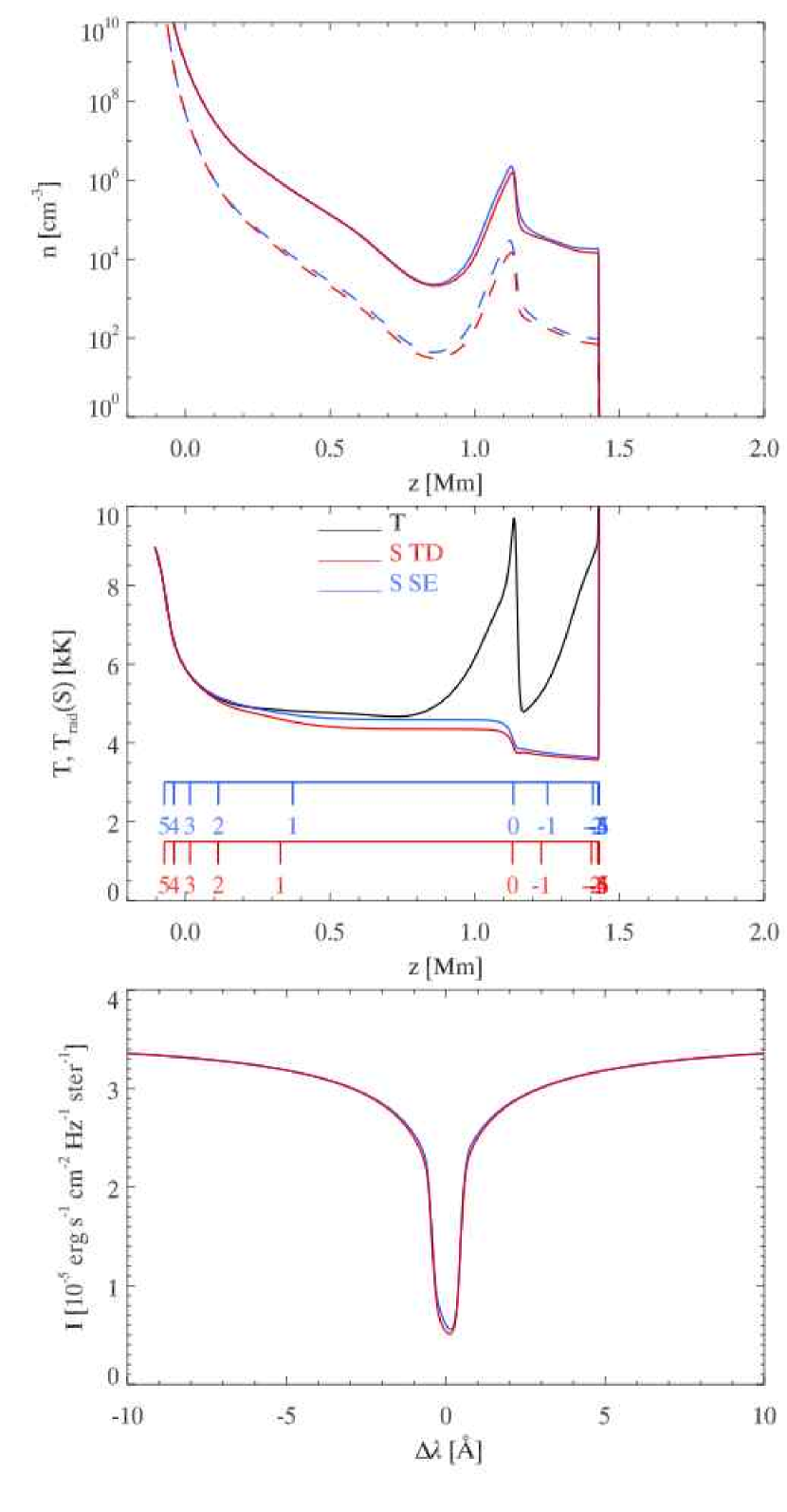
To investigate the effect of non-equilibrium radiative transfer on the formation of the H $\alpha$ line we use a time-series of hydrodynamical snapshots computed with the RADYN code (Carlsson & Stein, 1992, 1995, 1997, 2002).

This code solves the equations of conservation of mass, momentum, energy and mass. In addition it solves the non-LTE radiative transfer problem including non-equilibrium rate equations for hydrogen, helium and calcium. It uses a 5-level plus continuum model atom for H I and Ca II, and a nine-level helium atom with 5, 3 and 1 levels in He I, He II and He III respectively. These equations are solved implicitly on an adaptive mesh that moves points to regions where high spatial resolution is required (Dorfi & Drury, 1987). RADYN solves the non-equilibrium radiative transfer problem for hydrogen self-consistently including its effect on the ionization balance and therefore on the EOS. It treats PRD effects in the Lyman lines rather crudely, by truncating the Lyman line profiles at 48 km s^-1 away from the line-center frequency. We show in Sec. 4 that this simple method has only a minor effect on the formation of H $\alpha$.

In our RADYN simulation the lower boundary is located just below the photosphere at a column mass of $8.1$ g cm^-2, roughly corresponding to $\tau_{500\mathrm{nm}}=16$. The upper boundary is located in the corona, at 10,000 km above the lower boundary. The bottom boundary is closed and driven with a prescribed velocity field derived from MDI observations of the Doppler shifts of the 676.78 nm Ni I line in a quiet sun region. This driver excites waves that travel upward and steepen into shocks. We ran the simulation for slightly more than 1 hour of solar time and saved output at 10 s intervals, yielding a series of 374 snapshots of both the hydrodynamical state and the pertinent radiative transfer quantities.

For each of these 1D snapshots we then solved the non-LTE radiative transfer problem for hydrogen assuming statistical equilibrium with the radiative transfer code MULTI (Carlsson, 1986) using identical hydrodynamic quantities (temperature, mass density, electron density and vertical velocity) and model atom. MULTI and RADYN have identical source code for the routines that compute the radiative transfer. We thus ensured that any differences in the results are caused by the change from non-equilibrium (NE) level populations to transfer assuming statistical equilibrium (SE), and not by differences in the numerical method.

Figure 1 compares the formation of the H $\alpha$ line between NE and SE calculations at $t=3740$ s. At this time there is a strong shock in the chromosphere, a circumstance which typically exhibits the largest differences in line formation between NE and SE. At times that the chromospheric temperature structure is smooth there is almost no difference between the two assumptions.

The top panel shows the population densities of its upper and lower level. In SE both populations are slightly higher than in the NE case. Their ratio is however nearly equal, leading to a very similar source function, as shown in the middle panel. The SE computation shows a slightly higher source function throughout the simulated chromosphere. The line-core optical depth scales are nearly equal. The bottom panel compares the line profiles. They are near-identical, except in the line core, where the SE intensity is larger, which reflects the higher source function.

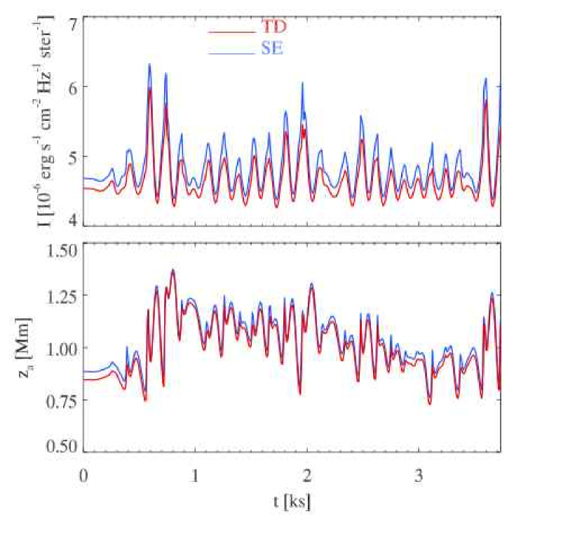
In Fig. 2 we compare the time evolution of the line-center intensity and the line-center average formation height $z_{\rm a}$. The latter is defined as

$$z_{\rm a}=\frac{\int_{z_{\rm b}}^{z_{\rm t}}z^{\prime}\chi S{\rm e}^{-\tau}{\rm d}z^{\prime}}{\int_{z_{\rm b}}^{z_{\rm t}}\chi S{\rm e}^{-\tau}{\rm d}z^{\prime}},$$ (1)

where $z_{\rm b}$ and $z_{\rm t}$ are the height of the bottom and top boundary in the model and $\chi$, $S$ and $\tau$ are the line-center opacity, source function and optical depth, respectively. The average formation height is in general not a good measure of where the H $\alpha$ line-core intensity is formed: the contribution functions are often multiply peaked and can be non-zero over ranges of more than 1 Mm. However, if the formation height range has to be quantified by one number, the average formation height is a better measure than the height of optical depth unity.

The curves for SE closely follow the corresponding curves for the full non-equilibrium solution. The SE intensity is consistently higher than the NE intensity, varying between 10% higher in the presence of shocks to only 2% higher during inter-shock phases. The SE average formation height is typically 30 km higher during inter-shock phases, and 80 km higher during shock passages. Both the differences in intensity and average formation height are much smaller than the intrinsic variability caused by the changing state of the atmosphere.

Therefore, we conclude that it is possible to assume SE for the radiative transfer of hydrogen, provided the temperature and electron density in the model atmosphere are computed with a simulation that includes the effect of non-equilibrium hydrogen ionization. The latter is essential: assuming statistical equilibrium when calculating the atmosphere leads to temperatures that can be more than 2000 K off and electron densities that can be even orders of magnitude off (Carlsson & Stein, 2002; Leenaarts et al., 2007).

This result is crucial in making it possible to compute realistic synthetic imagery in hydrogen lines from 3D simulations of the solar chromosphere. The detailed non-equilibrium treatment of radiative transfer as in RADYN is too computationally demanding in multi-dimensional geometry. It is, however, possible to compute the non-equilibrium ionization balance of hydrogen and its effect on the equation-of-state using approximations that are efficient enough to be included in a 3D MHD code.

3. 3D simulation snapshot and 3D radiative transfer

Figure 3.— Characterization of the Bifrost snapshot. Upper left: vertically emergent intensity in the continuum radiation bin. Upper right: Vertical magnetic field at $z=0$ Mm. Lower left: Gas temperature at $z=1.7$ Mm. Lower right: Angle of the magnetic field vector with the horizontal, with the red arrows indicating the direction of the horizontal component of the magnetic field.

In Sec. 4 and 5 we investigate the influence of partial redistribution in Lyman lines and 3D evaluation of the radiation field on the formation of H $\alpha$. We study these effects in a snapshot of a 3D radiation-MHD simulation computed with the Bifrost code.

Bifrost solves the equations of resistive MHD on a staggered Cartesian grid. In addition to this the code can solve various additional physical processes. The snapshot we are using was computed with the following additional physics: Optically thick radiative transfer in the photosphere and low chromosphere, parameterized radiative losses in the upper chromosphere, transition region and corona, thermal conduction along magnetic field lines and EOS that includes the effects of non-equilibrium ionization of hydrogen. As discussed in Sec. 2, the latter is of critical importance for the subsequent computation of solution of the radiative transfer problem for hydrogen.

This non-equilibrium EOS essentially solves the non-equilibrium rate equations for hydrogen with prescribed radiative rates, together with equations for energy, particle and charge conservation. By using prescribed rates there is no need to solve the transfer equation, and therefore the problem becomes computationally tractable in 3D simulations.

We refer the reader to Leenaarts et al. (2007) for more details about the non-equilibrium EOS, and to Gudiksen et al. (2011). for an extensive description of Bifrost.

Our simulation has a grid of $504\times 504\times 496$ grid cells, with an extent of $24\times 24\times 16.8$ Mm. In the vertical direction the grid extends from 2.4 Mm below to 14.4 Mm above average optical depth unity at 500 nm, encompassing the upper convection zone, photosphere, chromosphere and lower corona. The $x$ and $y$-axes are equidistant with a grid spacing of 48 km. The $z$-axis is non-equidistant. It has a grid spacing of 19 km between $z=-1$ and $z=5$ Mm, while the spacing increases towards the upper and lower boundaries to a maximum of 98 km at the coronal boundary. The magnetic field has a predominantly bipolar structure, that manifests itself in the photosphere as two clusters of magnetic concentrations of opposite polarity. The magnetic field was introduced into a relaxed hydrodynamical simulation through specifying the vertical magnetic field at the bottom boundary with a potential field extrapolation giving the magnetic field throughout the box. The field at the bottom boundary was given with an averaged signed field of zero and two patches of opposite polarity separated by 8 Mm. The simulation ran for 3000 s before switching on hydrogen non-equilibrium ionization. The snapshot we analyze is after 850 s with hydrogen non-equilibrium ionization.

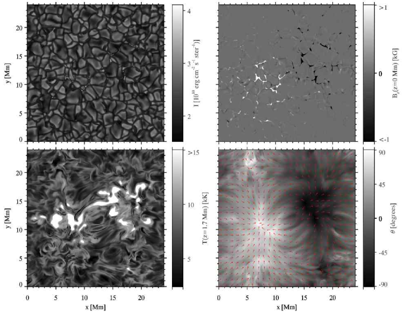
The average unsigned magnetic field strength at $z=0$ Mm in the snapshot we selected is 50 G. The snapshot is further characterized in Fig. 3. The upper-left panel displays the vertically emergent intensity in the continuum radiation bin. It shows granules and some bright intergranular structures that correspond to kG magnetic field concentrations as can be seen by comparing with the upper-right panel, which shows the vertical magnetic field strength at $z=0$ Mm. The two clusters of opposite polarity field stand out in black and white. The lower left panel shows the gas temperature in the chromosphere at a height of 1.7 Mm. The corona dips down to below this height above the photospheric magnetic field concentrations. Between the magnetic patches the temperature shows filamentary structure that follows the general orientation of the magnetic field. This can be seen in the lower-right panel, that shows the angle of the magnetic field vector with the horizontal, together with arrows pointing in the direction of the horizontal component of the field, also at $z=1.7$ Mm.

We performed the radiative transfer computations based on this snapshot with the Multi3d code (Leenaarts & Carlsson, 2009). This is a radiative transfer code capable of handling 3D model atmospheres. It can evaluate the radiation field for each column of the atmosphere separately (column-by-column plane-parallel approximation), or it can do so in full 3D, taking the horizontal structure into account.

Multi3d employs the accelerated lambda iteration method developed by Rybicki & Hummer (1992) with the extension to treat effects of partial frequency redistribution using the angle-averaged approximation by Uitenbroek (2001). In order to make the 3D radiative transfer problem computationally tractable we halved the horizontal resolution of the MHD snapshot and resampled the vertical grid to 200 equidistant points between $z=-0.5$ Mm and $z=5.5$ Mm to cover just the formation range of the various hydrogen transitions. For the radiative transfer computations we thus had a horizontal resolution of 96 km and a vertical resolution of 32 km.

We used a 5-level plus continuum hydrogen model atom. For computations assuming 1D plane-parallel geometry we used a 5-point Gauss-Legendre quadrature to compute the angle integration for each ray direction (so 10 rays in total) for the radiation field. For full 3D computations we employed the A4 set of Carlson (1963) with 3 rays per octant, and thus 24 rays in total. Multi3d does not include an equation for charge conservation. The non-LTE proton density we obtained is larger than the electron density at certain locations in the model atmosphere.

4. Influence of PRD in Lyman lines on H $\alpha$

Figure 4.— Comparison of H $\alpha$ line formation between various methods to treat radiative transfer in the Lyman-$\alpha$ and $\beta$ lines in a column of a 3D model atmosphere. In all panels the red curve indicate results obtained with angle-averaged PRD, orange with CRD, green with a Doppler profile and blue with a truncated Voigt profile. Top: optical depth versus height, the thin horizontal lines indicate $\tau$ equals 0.1,1 and 10, to guide the eye. Middle: gas temperature (black curve) versus height, with the total source function overplotted. Bottom: contribution function to intensity of the H $\alpha$ line center versus height. The thin horizontal line indicates ${\rm d}I/{\rm d}z=0$ to guide the eye. The average formation height is indicated by the triangles. Emergent line profiles for this atmosphere are shown in Fig. 5.

Figure 5.— Comparison of the H $\alpha$ line profile computed with the Lyman-$\alpha$ and $\beta$ lines treated with angle-averaged PRD (red), CRD (orange), a Doppler profile (green) and a truncated Voigt profile (blue). Details on how the line core is formed are shown in Fig. 4.

Figure 6.— Comparison of the H $\alpha$ line core formation with the Lyman-$\alpha$ and $\beta$ lines treated with angle-averaged PRD (red), CRD (orange), a Doppler profile (green) and a truncated Voigt profile (blue) in a 2D slice of a 3D radiation-MHD snapshot computed with Bifrost. Top panel: line core intensity versus spatial location. Bottom panel: average formation height versus spatial location. The stars indicate the column used in Figs. 4 and 5

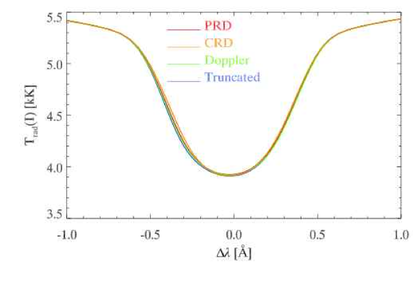
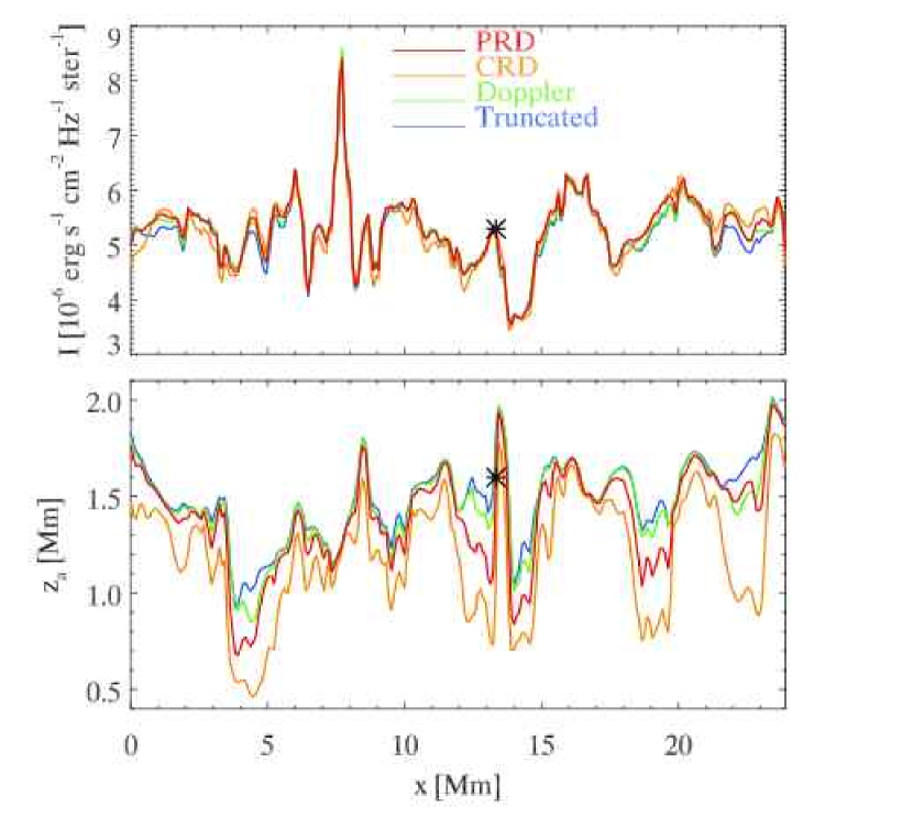
The Lyman lines of hydrogen are strongly affected by partial redistribution of photons over the line profile (PRD, e.g., Milkey & Mihalas, 1973; Vernazza et al., 1981). The Lyman line transfer affects the atomic level populations and therefore also the formation of the H $\alpha$ line. The computation of PRD effects in a three-dimensional atmosphere is currently unfeasible. This is partly due to the increase in computational cost compared to using the simplifying assumption of complete redistribution of photons over the line profile (CRD), and partly due to algorithm stability: the strong gradients present in MHD models very often lead to non-convergence of the $\Lambda$-iterations. We therefore investigated the effect of various approximations to PRD effects in the Lyman lines, in the hope of finding a simple recipe that has the same influence on the formation H $\alpha$ as PRD.

Inspired by Milkey & Mihalas (1973) and Avrett & Vernazza (1977) we compared four different treatments of the Lyman-$\alpha$ and $\beta$ lines: using angle-averaged PRD with a Voigt profile (hereafter ‘PRD case’), CRD with a Voigt profile (‘CRD case’), CRD with a Voigt profile truncated at 48 km s^-1 away from line center (‘truncated case’) and CRD with a Gaussian profile with Doppler broadening only (‘Doppler case’).

We took an $xz$-slice from the 3D Bifrost snapshot at $y=0$ Mm and solved the SE radiative transfer problem for hydrogen with Multi3d for each of the four different approximations, but otherwise identical input data. Each of the 252 columns was treated as a plane-parallel atmosphere. It turned out that the differences between the various cases showed behavior common to nearly all columns. We therefore show the results for one representative column only in Figs. 4 and 5.

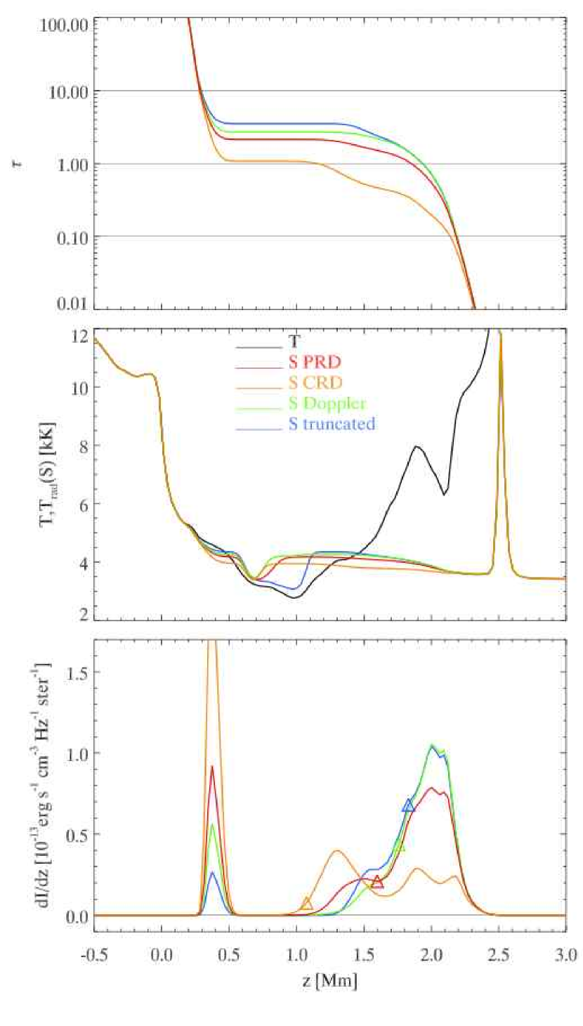
The top panel of Fig. 4 shows the optical depth as function of height for the various cases. The CRD case shows the lowest optical depth of the H $\alpha$ core at any given height, the truncated case the highest; the Doppler case is closest to the PRD case. In all cases there is no increase in optical depth with geometrical depth around $z=0.8$ Mm, indicating the ‘opacity gap’ typical of lines with an excited state as a lower level (Leenaarts et al., 2006). This can be seen in observations when stepping through a series of H $\alpha$ images at successively larger wavelength offset from line center, where the overall appearance jumps from high-chromospheric structure to photospheric granulation, without intermediate reversed granulation such as in the Ca II H line.

The ordering of the optical depth scales can be explained in terms of the thermalization depths of the Lyman-$\alpha$ line, or in other terms, as the probability in photon escape in the line wing (cf. Mihalas, 1978). The Doppler and truncated case have a very weak or no line wing, and therefore a low thermalization depth and few line photons escape through the line wings. In contrast, the Voigt case has prominent wings, a large thermalization depth and a fraction of the line photons escape into space through the wings. Therefore the Lyman-$\alpha$ line has a larger net downward rate and hence lower $n=2$ population and hence lower H $\alpha$ opacity in the Voigt case than in the Doppler and truncated cases. The PRD case is intermediate: Lyman-$\alpha$ and Lyman-$\beta$ behave more like Doppler lines in the upper chromosphere and more like a Voigt lines deeper down in the atmosphere.

The middle panel of Fig. 4 shows a comparison of the gas temperature and the total source function $S$ in the H $\alpha$ line core. The temperature drops down from the photosphere to a minimum at $z=1.25$ Mm, and then slowly increases to transition-region temperatures, with a dip at $z=2.0$ Mm. All source functions show $S=B$ (with $B$ the Planck function) up to $z=0.2$ Mm after which they decouple from the local temperature. The dips in the source functions at around $z=0.8$ Mm are caused by the very low line opacity causing the background source function to dominate the total source function. The large spike at $z=2.5$ Mm is likewise caused by the background processes and plays no role in the formation of the line. Except where the background source function is appreciable, in the core-forming region ($0.3<z<2.5$ Mm) the truncated and Doppler cases show a larger source function than in PRD. The CRD case a lower source function. The bottom panel shows the contribution function (CF) to intensity. All CFs are multiple-peaked and very wide, being non-zero over a height range of 2 Mm. The CRD case has the lowest average formation height ($z_{\rm a}$, indicated by a triangle), the truncated case the highest.

Fig. 5 shows the vertically emergent line profile for the same column as shown in Fig.4. The profiles are identical in the line wing. In the $\pm 0.6$ Å around line center the differences are small but visible.

Table 1Comparison of PRD approximations

Case	$<I/I_{\mathrm{PRD}}-1>$	$<z_{\rm a}-z_{\mathrm{a,PRD}}>$ (km)
Voigt	0.026	-203
Truncated	0.019	96
Doppler	0.011	65

The top panel of Fig. 6 compares the variation of the line-core intensity and average formation height for all columns in the $xz$-slice. The variations of the H $\alpha$ intensity due to the various PRD approximations in Ly-$\alpha$ and Ly-$\beta$ are much smaller than the variations due to the different atmospheric properties. Table 1 compares the relative difference in line core intensity between the various approximations and the PRD case. The Doppler case gives the best approximation to the PRD case, with on average only 1.1% difference in line-core intensity.

The bottom panel similarly compares the average formation height. Here the variations caused by the various PRD approximations are larger. The truncated case yields the highest $z_{\rm a}$, followed by the Doppler case, the PRD case, and lowest, the CRD case. As can be seen in Table 1, the Doppler case approximates the PRD case best, with on average a 64 km larger formation height. The differences between the Doppler and PRD cases are large where $z_{\rm a}$ is small, for example at $x=4$ Mm in the lower panel of 6; they are small where $z_{\rm a}$ is large, such as at $x=1$ Mm.

From the above analysis we conclude that it is possible to use Doppler profiles in the Lyman-$\alpha$ and $\beta$ lines without significantly influencing the formation of H $\alpha$.

5. The influence of 3D transfer on H $\alpha$

Figure 7.— Comparison of H $\alpha$ line-core formation between full 3D radiative transfer (left-hand column) and treatment of each column in the snapshot as a plane-parallel atmosphere (right-hand column). First row: vertically emergent intensity. Second row: average formation height. Third row: angle-averaged radiation field at optical depth unity.

The conclusions of Sec 2 and 4, namely that it is possible to model H $\alpha$ line formation assuming statistical equilibrium and approximating PRD effects in the Lyman lines, makes it numerically feasible to perform 3D radiative transfer. Effects from 3D radiative transfer are expected to be important for strongly scattering lines like Na I D₁ (Leenaarts et al., 2010) but not so important for lines that have a strong coupling of the source function to the temperature like the Ca II infrared triplet lines (Leenaarts & Carlsson, 2009). The H $\alpha$ line is strongly scattering as can be seen in the interesting comparison of Ca II 8542 to H $\alpha$ formation in Fig. 8 of Cauzzi et al. (2009). The H $\alpha$ source function decouples from the temperature already in the photosphere in the 1D FAL model C of Fontenla et al. (1993) and is afterwards essentially equal to the angle-averaged radiation field. An important corollary of this is that the line-core intensity is determined mainly by the photospheric temperature, i.e.,the line-core response function to temperature peaks in the photosphere (Socas-Navarro & Uitenbroek, 2004; Uitenbroek, 2006a).

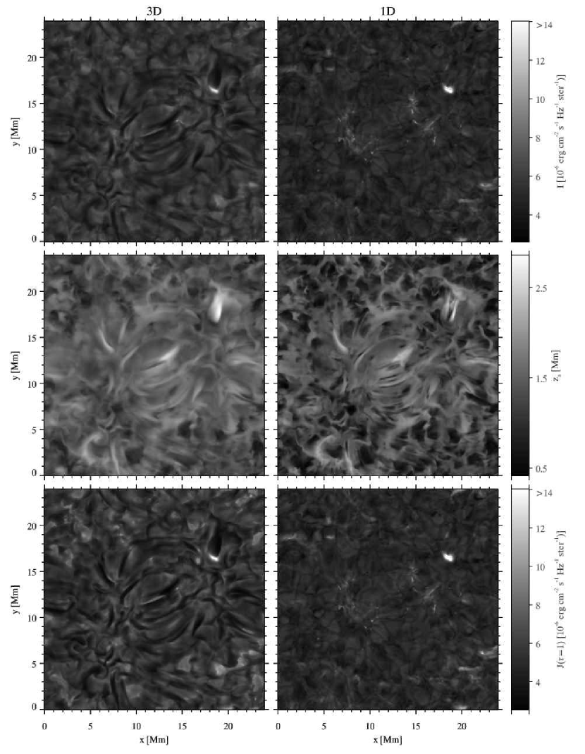
We therefore solved the radiative transfer problem for hydrogen in our entire Bifrost snapshot twice, once with full 3D transfer, and once treating each column as a plane-parallel atmosphere (hereafter called 1D transfer). We assumed SE and the approximation to PRD from Sec. 4. No microturbulence was added. The results are shown in Fig. 7.

The top row compares the vertically emergent intensity between 3D and 1D. They show a starkly different scene. The 3D computation shows striking, predominantly dark, fibril-like features emanating from the photospheric field concentrations, which appear to follow the magnetic field lines (compare to Fig. 3). They are superimposed on a background of irregularly shaped patches of roughly 2 Mm diameter of varying brightness. The 1D computation instead shows a distinctly photospheric scene with granulation and magnetic bright points, much more reminiscent of observations in the line wing.

The second row shows the average formation height. The 3D image shows that the structures that appear dark in the line-core image are formed highest. The irregular background in the intensity image has a lower $z_{\rm a}$. In the 1D case the situation is largely the same, except that it shows more small scale structure (due to the absence of smoothing 3D radiation effects on the opacity) and the patches of small $z_{\rm a}$ away from the magnetic concentrations.

The bottom row shows the angle-averaged line-core radiation field $J_{\nu 0}$ at the local optical depth unity. Both the 1D and 3D images appear very similar to the corresponding intensity images. This validates the Eddington-Barbier (EB) approximation $I_{\nu 0}(\mu)\approxeq S_{\nu 0}(\tau=\mu)$ for vertical rays ($\mu=1$), and also that the core source function is set by scattering ($S_{\nu 0}(\tau=1)\approxeq J_{\nu 0}(\tau=1)$).

This also explains why the 1D intensity image shows granulation and bright points. The H $\alpha$ source function at optical depth unity is given by the $J_{\nu 0}(\tau=1)$, which in turn is mainly set in the photosphere. In 1D there is no smoothing of the radiation field, and $J_{\nu 0}(\tau=1)$ in a given column correlates strongly with temperature at the thermalization depth in that column. This temperature is lowest in intergranular lanes, higher inside granules and highest in magnetic elements. The resulting image therefore shows the structure of the photosphere, even though optical depth unity lies much higher.

We conclude that it is essential to include 3D radiative transfer effects in the formation of the H $\alpha$ line core. In the next section we analyze the results of our 3D computation in more detail.

6. Analysis of the 3D computation

6.1. H $\alpha$ core intensity correlates with average formation height

Figure 8.— Panels, from top to bottom: (1) Probability density function (PDF) of the source function at optical depth unity as function of emergent H $\alpha$ intensity in the line-core. The grey line indicates $S=I$. (2) PDF of the angle-averaged radiation field $J$ as function of height. The white curve shows the horizontal average of $J$ as function of height. (3) PDF of the line-core optical depth unity height as function of emergent H $\alpha$ intensity. The gray curve displays the same quantity as the white curve from panel 2, but transposed to account for the different arrangement of the axes. (4) PDF of the average formation height as function of emergent H $\alpha$ intensity. The gray curve is the same as for panel 3. All panels have each column individually scaled to maximum contrast for improved readability.

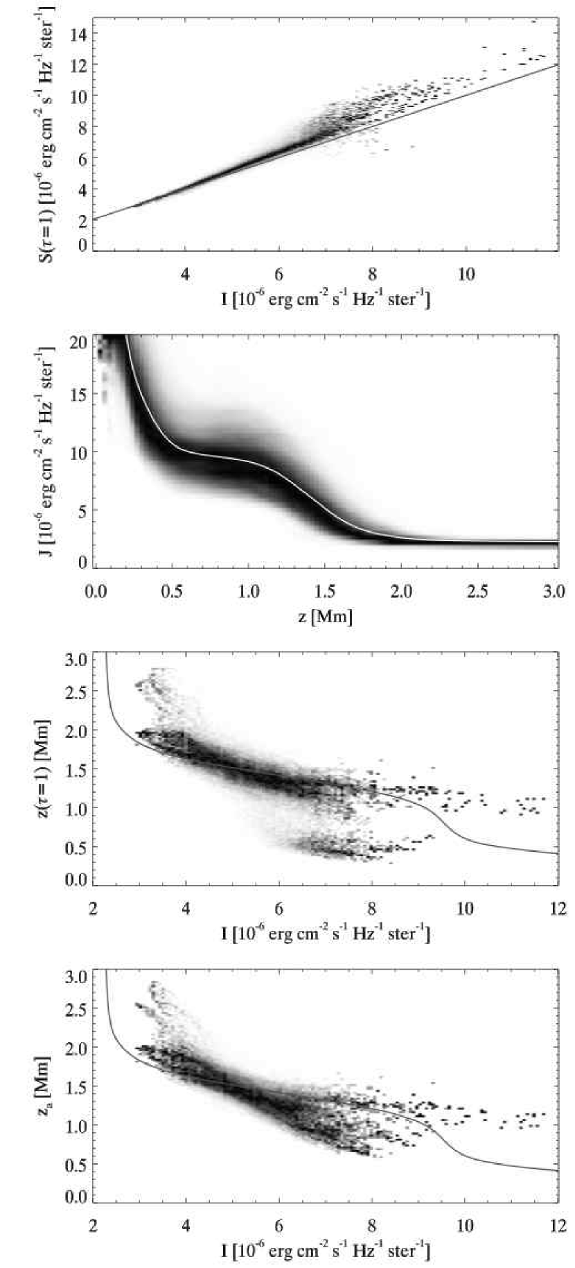
Fig. 7 suggests a correlation between H $\alpha$ intensity and average formation height for the 3D computation. In Fig. 8 we investigate the cause of this effect. The top panel shows the probability density function (PDF) of the line-core source function at optical depth unity as function of emergent H $\alpha$ intensity in the line core. It confirms that the Eddington-Barbier relation is valid. The second panel shows the PDF of $J_{\nu 0}$ as function of height. There is a rather small spread of $J_{\nu 0}$ around the horizontal average of the angle-averaged radiation field $<J_{\nu 0}>_{xy}$. The latter is a decreasing function of height up to 2 Mm height, after which it becomes flat.

The third panel shows the PDF of the line core optical depth unity height as function of emergent intensity. There is a strong correlation between the two quantities between $I$=4$\times$10^-6 and $I$=7$\times$10^-6 erg cm^-2 s^-1 Hz^-1 ster^-1. At lower intensity the correlation shows two protrusions with a steeper slope. Between $I$=7$\times$10^-6 and $I$=8$\times$ 10^-6 erg cm^-2 s^-1 Hz^-1 ster^-1 the distribution is bimodal, with maxima at around $z=0.5$ Mm and $z=1.3$ Mm. This bimodality is caused by the mid-chromospheric opacity gap: this gap is typically located around optical depth unity for those emergent intensities. Depending on whether $\tau=1$ is reached above or below this gap, a given column in the atmosphere contributes to the low or the high cluster of points in the PDF.

At even higher emergent intensities the $\tau=1$ height appears independent of the intensity. The number of columns with this intensity is small, so it is unclear whether this is significant. The bimodality can be largely removed by using the average formation height instead of the height of optical depth unity. The former is much less sensitive to the location of the $\tau=1$ height than the latter. This is shown in the bottom panel.

The correlation between I and $z_{\rm a}$ (or $z(\tau=1)$) can now easily be explained: The Eddington-Barbier approximation is valid, and scattering ensures $S_{\nu 0}=J_{\nu 0}$. The radiation field $J_{\nu 0}$ shows relatively little variation with horizontal position and its horizontal average is monotonically decreasing with height. Therefore, larger average formation height leads to lower intensity. Above $z=1.7$ Mm the radiation field is approximately constant with height and the formation height and emergent intensity are no longer correlated.

6.2. H $\alpha$ line-core width correlates with temperature

Figure 9.— Comparison of line-core width (top) and temperature averaged between $\tau=0.5$ and $\tau=5$ at the wavelength of the profile minimum (bottom).

Figure 10.— Probability density function (PDF) of the temperature averaged between $\tau=0.5$ and $\tau=5$ at the wavelength of the profile minimum against the line-core width, after smoothing with a $3\times 3$ moving boxcar average. The black curve is a quadratic fit to the data.

Because of the low mass of the hydrogen atom it is expected that the width of the H $\alpha$ line core is sensitive to the temperature in the line forming region. Because the Doppler speed ($\sqrt{2kT/m_{{\rm H}}}=13$  km s^-1 for $T=10$ kK) is comparable to or larger than typical gas velocities in the chromosphere, the core width is not very sensitive to velocity gradients along the line-of-sight in the line forming region.

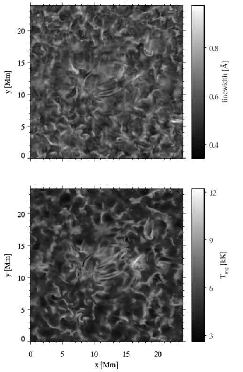
Because we are interested in a diagnostic of the chromospheric temperature we choose to measure the line width close to the line core. For each pixel in our synthetic image we determined the profile minimum and maximum ($I_{\mathrm{min}}$ and $I_{\mathrm{max}}$) and then defined the core width as the wavelength difference between the intersections of the profile and the line $I=I_{\mathrm{min}}+0.1(I_{\mathrm{max}}-I_{\mathrm{min}})$. We then computed for each pixel the temperature averaged over the height range between $\tau=0.5$ and $\tau=5$ at the wavelength of the profile minimum. The height range was extended to larger optical depths because one looks deeper in the atmosphere at the wavelengths that define the line-core width than in the line-core.

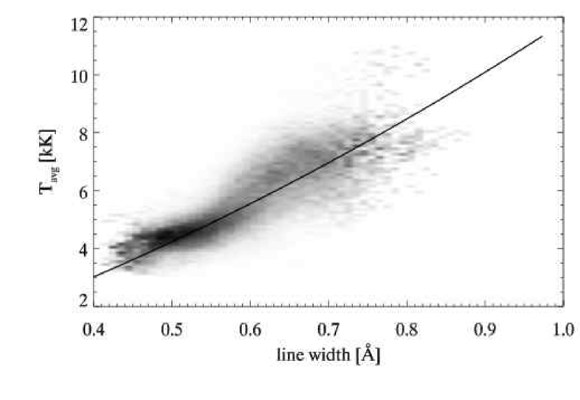
The results are shown in Fig. 9. Comparison of the two panels shows that there is a decent correspondence between large width and large average temperature, but in general no clear correspondence for pixels with low width and low temperature. The darker areas in the upper panel show a granulation pattern (compare with Fig. 3), while the average temperature panel does not. The notable exception are the dark elongated structures which clearly show up near the center of both panels. Fig. 10 shows the PDF of the average temperature versus the core width after smoothing both with a $3\times 3$ moving boxcar average. The averaging serves to remove outliers in the correlation.

This figure confirms the impression obtained from the images: the two quantities are quite well correlated at higher values, but in the low to intermediate regime (below a line width of 0.6 Å) the correlation is rather weak.

The correlation can be understood using optically thick line formation,the Eddington-Barbier approximation and the fact that the run of source function with height is monotonically decreasing and rather similar for each column (cf. Fig. 8). Because Eddington-Barbier is valid, one looks deeper and deeper into the atmosphere as one moves away from the line center and one sees a higher and higher source function and hence emergent intensity. A low temperature means a narrow absorption profile, hence steep gradient of the height of optical depth unity with wavelength and therefore a narrow line. At higher temperature the absorption profile is wider, a less steep ${\rm d}z(\tau=1)/d\lambda$ gradient and therefore a wider line. The actual line width at any given location therefore depends on both the temperature, and the gradient of the source function with optical depth in the line forming region. Variation in the latter is the main cause of the scatter in Fig. 9.

6.3. No correlation of H $\alpha$ opacity with temperature in the upper chromosphere

Figure 11.— PDF of the relative occupation of the H $\alpha$ lower level as function of the gas temperature at heights between 1 Mm and 3 Mm. The black curve indicates the Saha-Boltzmann occupation for the average electron density over this height range, 3.65$\times$10¹⁰ g cm^-3. Each column has been scaled to maximum contrast.

Figure 12.— PDF of the column mass at the H $\alpha$ line-core $\tau$=1 height as function of the $\tau$=1 height. Each column has been scaled to maximum contrast. The black curve represents the horizontal average of the column mass.

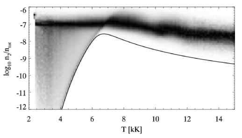
The H $\alpha$ line opacity is often considered to be sensitive to the temperature. This is true in the photosphere and lower chromosphere where the level populations are close to LTE, but does not hold in the upper chromosphere. There the H $\alpha$ opacity per gram is determined by the ionization degree (Carlsson & Stein, 2002) and the radiation field. The ionization degree is insensitive to temperature variations over time due to the long ionization-recombination timescale. The radiation field is non-locally determined and therefore independent of the local temperature.

We demonstrate this in Fig. 11. It shows the $n$=2 population relative to the total (neutral plus ionized) hydrogen density for each grid point in our simulation with a height between 1 Mm and 3 Mm. At temperatures below 4 kK the distribution is very wide, at higher temperatures the distribution narrows considerably and its peak value varies little over the whole temperature range. The black curve indicates the LTE value of the relative occupation number, which varies by many orders of magnitude.

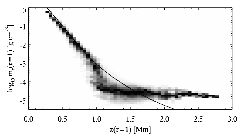
The temperature-insensitivity of the upper-chromospheric opacity means the opacity is mainly determined by the mass density. Therefore, the optical depth scale in the upper chromosphere is proportional to the column mass. This is shown in Fig. 12, where we show the PDF of the column mass at the $\tau$=1 height as function of the $\tau$=1 height. It shows that if the $\tau$=1 height is above 1.2 Mm, it has a constant column mass of roughly 3$\times$10^-5 g cm².

At lower heights the opacity is sensitive to both the temperature and the mass density. The column mass at the lower lying $\tau$=1 heights is therefore no longer constant, and is close to the horizontal average of the column mass instead.

6.4. Fibril-like structures align with the magnetic field in a low $\beta$ environment

Figure 13.— Image of the line-center intensity. Red arrows indicate the direction of the horizontal component of the magnetic field at the average formation height. Arrow length is proportional to field strength. The contours indicate values of plasma $\beta$ equals 0.01 (white) and 0.1 (green) at the average formation height. The white tick marks indicate the cut used in Fig. 14. White crosses indicate locations of fibrils crossing this cut. This figure is best viewed by magnifying the PDF file on a computer screen.

Chromospheric fibrils in H $\alpha$ are associated with the presence of photospheric magnetic elements and are conventionally thought to trace out magnetic field lines, but this has so far only been shown for the Ca II 8542 Å line (de la Cruz Rodríguez & Socas-Navarro, 2011)

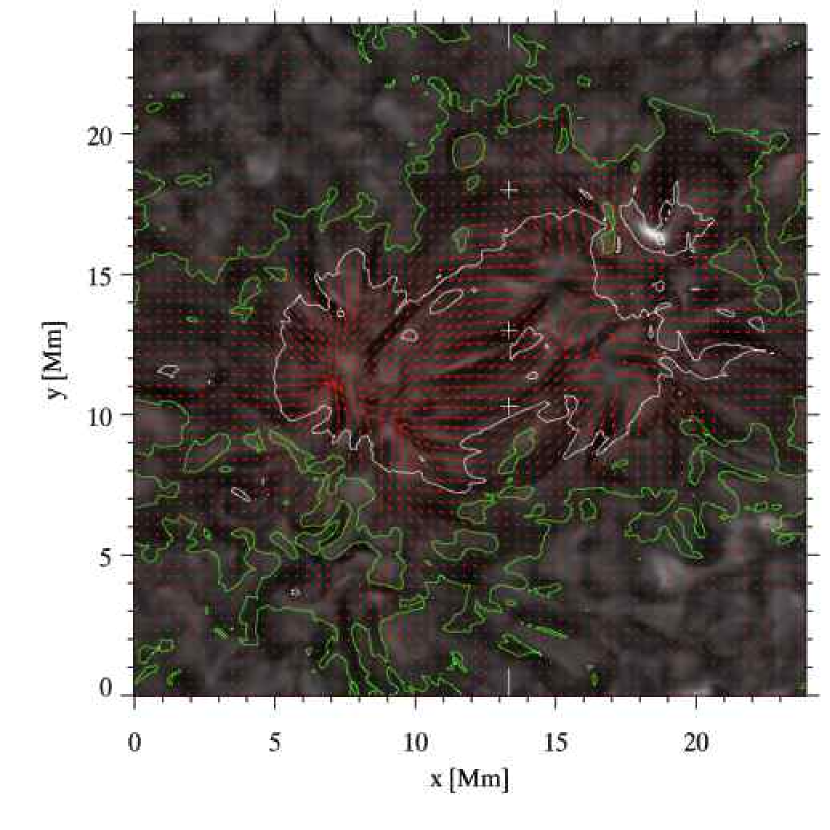
Fig. 13 investigates the alignment of the magnetic field in the model atmosphere with the dark fibril-like structures in the H $\alpha$ line-core. The figure shows the emergent intensity with the horizontal magnetic field direction and the plasma $\beta$ (ratio of gas pressure over magnetic pressure) at the average formation height overplotted. The fibrils are mainly located within the $\beta=0.01$ contour, between the photospheric field concentrations of opposite polarity. These fibrils are closely following the magnetic field direction. Outside the $\beta=0.1$ contour there are virtually no fibril-like structures and the image shows a more grainy appearance. Note that the semi-transparent fibrils at $(x,y)=(13.3,18)$ Mm (around the upper white cross, best seen in the upper-left panel of Fig. 7) also align with the field.

6.5. Fibril-like structures caused by field-aligned density ridges

Figure 14.— Vertical slice through the atmosphere along the cut indicated in Fig. 13. Vertical black lines indicate the positions of dark fibrils marked with white crosses in Fig. 13. The white or red curve indicates the average formation height. a: gas temperature; b: mass density; c: vertical velocity; d: magnetic field strength. The red, green and blue contours indicate plasma $\beta$ equals 1,0.1 and 0.01 respectively. ; e: emergent line-center intensity f: angle-averaged line-center radiation field; g: contribution function to line-center intensity, each column scaled to maximum contrast; h: line-center source function.

Figure 15.— Display of ridge-like dark fibrils. Left panel: emergent intensity in the central part of the atmosphere. Middle panel: 3D surface plot of the average formation height, with the color coding indicating the vertically emergent intensity. Right panel: iso-surface of the mass density at $\rho=10^{-11}$ g cm^-3, with the color coding again indicating the vertically emergent intensity. The dark fibrils follow ridges of enhanced chromospheric mass density.

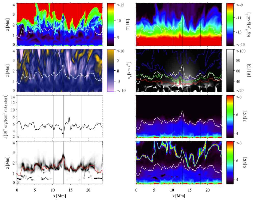
We now further investigate the cause of the dark structures by showing an $yz$ slice through the atmosphere along the cut indicated in Fig. 13. The panels a–d of Fig. 14 show the temperature, mass density, vertical velocity and magnetic field strength. The fibril locations (indicated by the vertical lines) do not show a particular correlation with temperature and vertical velocity. Panel d again shows they are located in an area with high magnetic field and low plasma $\beta$. The mass density panel clearly shows that the fibrils are located where there is enhanced chromospheric density, which causes the average formation height to be larger and thus the emergent intensity to be lower (see Sec. 6.1).

Panels e–h show the radiative transfer properties of the slice. The fibrils appear as local minima in the intensity. In the core-forming region the source function is nearly equal to the angle-averaged radiation field.

The contribution functions show a great variation in height of formation, exhibit multiple peaks and typical extended upward streaks. Away from the regions with strong field the average formation height tends to be lower, with a strong contribution from around 0.5 Mm height. In regions with stronger fields, there is no pronounced contribution from this depth in the atmosphere.

Fig. 15 shows the relation between H $\alpha$ intensity, average formation height and chromospheric mass density structure. The left panel shows the emergent line-core intensity in a subfield of the snapshot that shows fibrils. The middle panel shows a 3D rendering of the average formation height surface, with the emergent intensity as the image on the surface. It shows the dark fibrils as ridges with a large average formation height. Finally, the right panel shows a 3D representation of the iso-surface of the mass density at $\rho=10^{-11}$ g cm^-3, again with the emergent intensity as the image on the surface. Wherever the average formation height shows a ridge, there is a corresponding height increase in the density iso-surface. Even though the exact shapes are not identical, it is obvious that the dark fibrils between the two clusters of opposite polarity field are caused by ridges of enhanced chromospheric mass density. The fibrils that point away from both magnetic field concentrations are also co-spatial with locations of increased mass density, but because they are shorter, they appear more as mountains than as ridges.

7. Comparison with observations

Figure 16.— H $\alpha$ observations obtained with the Swedish Solar Telescope. a: intensity in the blue wing at 2.1 Å from line center; b: line-core width; c: line-center intensity; d: average gas temperature in the formation height range as determined from the fit of Fig. 10.

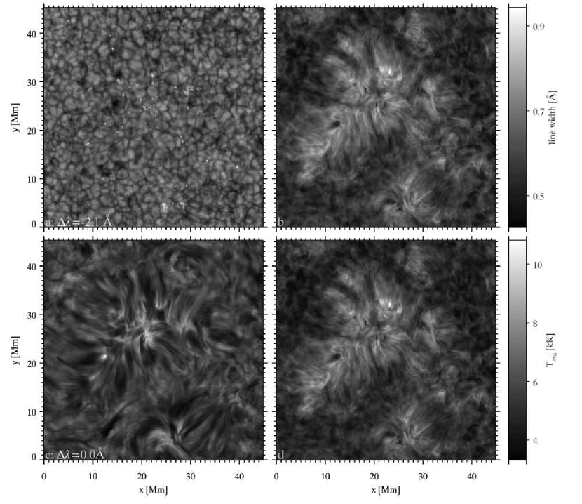
Fig. 16 shows observations of a quiet sun region taken in the H $\alpha$ line. The observations were obtained with the CRisp Imaging SpectroPolarimeter (CRISP, Scharmer et al., 2008) at the Swedish 1-m Solar Telescope (SST, Scharmer et al., 2003a) on La Palma on May 5,2011 at 7:53 UT. The H $\alpha$ spectral line was sampled with 35 line positions, from $-$2.064 Å to $+$1.290 Å, and equidistant 86 mÅ stepping between $\pm$1.290 Å. The time to complete a full line scan was 8 s. The target area was a quiet 60$\times$60″region at disk center centered at $(x,y)=(19$″,$5$″$)$. The seeing conditions were very good and the data quality benefited from the SST adaptive optics system (Scharmer et al., 2003b) and Multi-Object Multi-Frame Blind Deconvolution (MOMFBD, van Noort et al., 2005) image restoration. For more details on the data processing, we refer to Rouppe van der Voort et al. (2009).

Panel a shows the blue-wing image. It shows granulation and bright points associated with magnetic concentrations. Panel c shows the line-center image. There are two clusters of fibrils centered at (27,7) Mm and (23,27) Mm pointing away from the photospheric bright points. There appear to be no fibrils connecting the clusters, so it is likely the magnetic field in the image is largely unipolar. At larger distances from the bright points the line-core shows a more grainy appearance without the elongated structures. This is seen most clearly in the upper-left corner and close to the edge of the image at the right-hand side.

The synthetic line-core image in the upper left panel of Fig. 7 shows a similar structure, it shows fibril-like structure close to the photospheric magnetic concentrations and grainy structure elsewhere. The simulations lack the dense packing of the fibrils in the observations and shows typically shorter fibril-like structures. The width of the dark fibrils in the observations are similar to the width of the dark fibril-like structures in the simulations.

Panel b shows the line-core width, determined in the same way as for the simulations (see Sec. 6.2). The fibrils show largest width. The areas with lower width do not show a granulation pattern, instead it shows a pattern reminiscent of reversed granulation or acoustic shocks. Comparison of panel b and Fig. 9) shows that the synthetic fibril-like structures show up much less in the line-width measurement than the observed fibrils. The signature of the granulation pattern in the simulations shows that the simulated internetwork has a lower H $\alpha$ opacity than the sun. The range of line-core widths in the simulation is very similar to the one measured in the observations.

Panel d finally shows the gas temperature derived from the core width assuming the fit from Fig. 10. It shows temperatures between 4 and 8 kK for internetwork areas. The fibrils have a higher temperature of around 10 kK. Note that the brightest patches in the line-core image do not correspond to the largest core width or derived temperature.

8. Discussion and Conclusions

We have presented results of a radiative transfer computation of the H $\alpha$ line based on a model atmosphere computed with a state-of-the-art radiation-MHD code. This is the first time that a simulation reproduces chromospheric fibril-like structures in synthetic observables.

The crucial ingredient for the formation of fibril-like structures is the full 3D evaluation of the transfer equation. The H $\alpha$ source function decouples from the temperature already in the photosphere and the source function at optical depth unity in the chromosphere is therefore set by radiation emitted in a large volume and hence fairly smooth.

In our simulation the emergent line-core intensity correlates with the average formation height: the lower the intensity, the higher in the atmosphere the photons are originating. It is a very different explanation than the one that is typically assumed by cloud modeling, where variation in emergent intensity is assumed to be caused by varying thermodynamic properties in a cloud that modulate the intensity emitted by the photosphere below.

We expect that this intensity-formation-height correlation is also valid on the sun, as it is based only on the assumption that the H $\alpha$ line is strongly scattering within its formation height range, so that the source function is set by scattering and the angle-averaged radiation field shows relatively little variation with horizontal spatial position. However, the shape of the correlation curve depends on the exact run of the source function with height. The latter depends on the temperature at the thermalization depth and the chromospheric opacity. These will be different in, for example, internetwork, network or plage and different again in our simulation. When comparing intensities for small areas on the sun one can conclude that the lower the intensity the higher in the atmosphere one looks, but intensities in very different regions cannot be directly compared.

A largely similar argument holds for the correlation between line-core width and gas temperature. This correlation can be simply explained by optically thick line formation and the Eddington-Barbier approximation and is therefore doubtlessly valid on the sun too. The exact shape of the correlation depends on the variation of source function and opacity with height. The fit shown in Fig. 10 is therefore likely not universally valid.

In addition, the method is sensitive to velocity gradients that are of the same order as the line width. Such a gradient causes an increase in line width compared to an identical atmosphere without a velocity field. For example, the asymmetric profiles of ‘rapid blueshifted events’ (Rouppe van der Voort et al., 2009) would show up as having increased temperature using the core-width measure, without this necessarily being the case.

Still, if we assume it is valid and apply it, our observations yield internetwork temperatures compatible with radiation-MHD simulations of the internetwork chromosphere (Carlsson & Stein, 1995; Skartlien, 2000; Wedemeyer et al., 2004; Leenaarts et al., 2007). We find temperatures of 10 kK for H $\alpha$ fibrils. This is comparable to values found in many studies that use cloud modeling (e.g., Heinzel & Schmieder, 1994; Tsiropoula & Schmieder, 1997; Bostancı, 2011) However, all cloud modeling requires addition of a ‘microturbulent velocity’ of typically 5 to 15 km s^-1 as an ad hoc parameter to derive the temperature from the observed cloud model parameters. The profiles in our simulation have similar widths as the observations and yield similar temperatures without the need of invoking microturbulence.

The line formation properties of H $\alpha$ show a double character. At heights below 1 Mm its opacity is temperature-sensitive because of its excited lower level. At larger heights this temperature sensitivity disappears. There the opacity is instead mainly sensitive to density, much more akin to resonance lines, which have the ground state as a lower level.

Our simulation supports the commonly held notion that fibrils indeed trace the magnetic file. More precisely we show that the orientation of the fibril-like structures in the synthetic H $\alpha$ core image align with the horizontal component of the magnetic field at the average formation height computed for each pixel separately. This supports the practice of using H $\alpha$ imagery to constrain and test the quality of field extrapolations (e.g., Judge et al., 2010; Jing et al., 2011; Reardon et al., 2011).

The dark fibrils-like structures in the simulation are caused by ridge-like density enhancements in the chromosphere that lead to higher formation height and hence lower emergent intensity. It is unlikely the density ridges are the only way to create fibrils on the Sun. The simulation has a limited resolution and spatial extent and still lacks treatment of physical processes that might be important in the chromosphere, such as heating due to neutral-ion drag (Krasnoselskikh et al., 2010).

We can now answer the question what makes H $\alpha$ such a good line to observe the magnetic structure of the chromosphere. The main reason is that it happens to have so much opacity in the line core that it almost always forms in the low plasma beta regime where the magnetic field is the main structuring agent in the atmosphere. The low mass of the hydrogen atom makes the line wide, so that the fixed-wavelength line-core intensity is only weakly modulated by the velocity field. Instead, the correlation of formation height and intensity and the constant column mass at the $\tau$=1 height make the line-core intensity a tracer of the chromospheric mass density. It is the variation of the mass density caused by the magnetic field, waves and shocks that gives rise to the dramatic structures seen in H $\alpha$.

References

- Avrett & Vernazza (1977) Avrett, E. H. & Vernazza, J. E. 1977, in Bulletin of the American Astronomical Society, Vol. 9, Bulletin of the American Astronomical Society, 432
- Bostancı (2011) Bostancı, Z. F. 2011, Astronomische Nachrichten, 332, 815
- Carlson (1963) Carlson, B. G. 1963, Methods of Computational Physics, 1
- Carlsson (1986) Carlsson, M. 1986, Uppsala Astronomical Observatory Reports, 33
- Carlsson & Stein (1992) Carlsson, M. & Stein, R. F. 1992, ApJ, 397, L59
- Carlsson & Stein (1995) Carlsson, M. & Stein, R. F. 1995, ApJ, 440, L29
- Carlsson & Stein (1997) Carlsson, M. & Stein, R. F. 1997, ApJ, 481, 500
- Carlsson & Stein (2002) Carlsson, M. & Stein, R. F. 2002, ApJ, 572, 626
- Cauzzi et al. (2009) Cauzzi, G., Reardon, K., Rutten, R. J., Tritschler, A., & Uitenbroek, H. 2009, A&A, 503, 577
- de la Cruz Rodríguez & Socas-Navarro (2011) de la Cruz Rodríguez, J. & Socas-Navarro, H. 2011, A&A, 527, L8
- De Pontieu et al. (2007a) De Pontieu, B., Hansteen, V. H., Rouppe van der Voort, L., van Noort, M., & Carlsson, M. 2007a, ApJ, 655, 624
- De Pontieu et al. (2007b) De Pontieu, B., McIntosh, S. W., Carlsson, M., et al. 2007b, Science, 318, 1574
- Dorfi & Drury (1987) Dorfi, E. A. & Drury, L. O. 1987, Journal of Computational Physics, 69, 175
- Fontenla et al. (1993) Fontenla, J. M., Avrett, E. H., & Loeser, R. 1993, ApJ, 406, 319
- Gudiksen et al. (2011) Gudiksen, B. V., Carlsson, M., Hansteen, V. H., et al. 2011, A&A, 531, A154
- Hansteen (2004) Hansteen, V. H. 2004, in IAU Symposium, Vol. 223, Multi-Wavelength Investigations of Solar Activity, ed. A. V. Stepanov, E. E. Benevolenskaya, & A. G. Kosovichev, 385–386
- Hansteen et al. (2007) Hansteen, V. H., Carlsson, M., & Gudiksen, B. 2007, in Astronomical Society of the Pacific Conference Series, Vol. 368, The Physics of Chromospheric Plasmas, ed. P. Heinzel, I. Dorotovič, & R. J. Rutten, 107
- Hansteen et al. (2006) Hansteen, V. H., De Pontieu, B., Rouppe van der Voort, L., van Noort, M., & Carlsson, M. 2006, ApJ, 647, L73
- Heinzel & Schmieder (1994) Heinzel, P. & Schmieder, B. 1994, A&A, 282, 939
- Jing et al. (2011) Jing, J., Yuan, Y., Reardon, K., et al. 2011, ApJ, 739, 67
- Judge et al. (2010) Judge, P. G., Tritschler, A., Uitenbroek, H., et al. 2010, ApJ, 710, 1486
- Krasnoselskikh et al. (2010) Krasnoselskikh, V., Vekstein, G., Hudson, H. S., Bale, S. D., & Abbett, W. P. 2010, ApJ, 724, 1542
- Leenaarts (2010) Leenaarts, J. 2010, Mem. Soc. Astron. Italiana, 81, 576
- Leenaarts & Carlsson (2009) Leenaarts, J. & Carlsson, M. 2009, in Astronomical Society of the Pacific Conference Series, Vol. 415, Astronomical Society of the Pacific Conference Series, ed. B. Lites, M. Cheung, T. Magara, J. Mariska, & K. Reeves, 87
- Leenaarts et al. (2009) Leenaarts, J., Carlsson, M., Hansteen, V., & Rouppe van der Voort, L. 2009, ApJ, 694, L128
- Leenaarts et al. (2007) Leenaarts, J., Carlsson, M., Hansteen, V., & Rutten, R. J. 2007, A&A, 473, 625
- Leenaarts et al. (2010) Leenaarts, J., Rutten, R. J., Reardon, K., Carlsson, M., & Hansteen, V. 2010, ApJ, 709, 1362
- Leenaarts et al. (2006) Leenaarts, J., Rutten, R. J., Sütterlin, P., Carlsson, M., & Uitenbroek, H. 2006, A&A, 449, 1209
- Lockyer (1868) Lockyer, J. N. 1868, Royal Society of London Proceedings Series I, 17, 128
- Martínez-Sykora et al. (2008) Martínez-Sykora, J., Hansteen, V., & Carlsson, M. 2008, ApJ, 679, 871
- Martínez-Sykora et al. (2009a) Martínez-Sykora, J., Hansteen, V., & Carlsson, M. 2009a, ApJ, 702, 129
- Martínez-Sykora et al. (2009b) Martínez-Sykora, J., Hansteen, V., DePontieu, B., & Carlsson, M. 2009b, ApJ, 701, 1569
- Martínez-Sykora et al. (2011) Martínez-Sykora, J., Hansteen, V., & Moreno-Insertis, F. 2011, ApJ, 736, 9
- Mihalas (1978) Mihalas, D. 1978, Stellar atmospheres /2nd edition/ (San Francisco, W. H. Freeman and Co., 1978. 650 p.)
- Milkey & Mihalas (1973) Milkey, R. W. & Mihalas, D. 1973, ApJ, 185, 709
- Reardon et al. (2011) Reardon, K. P., Wang, Y.-M., Muglach, K., & Warren, H. P. 2011, ApJ, 742, 119
- Rouppe van der Voort et al. (2009) Rouppe van der Voort, L., Leenaarts, J., De Pontieu, B., Carlsson, M., & Vissers, G. 2009, ApJ, 705, 272
- Rutten (2008) Rutten, R. J. 2008, in Astronomical Society of the Pacific Conference Series, Vol. 397, First Results From Hinode, ed. S. A. Matthews, J. M. Davis, & L. K. Harra, 54
- Rutten (2010a) Rutten, R. J. 2010a, in Recent Advances in Spectroscopy Theoretical, Astrophysical and Experimental Perspectives, ed. R. K. Chaudhuri, M. V. Mekkaden, A. V. Raveendran, & A. Satya Narayanan , 163–175
- Rutten (2010b) Rutten, R. J. 2010b, Mem. Soc. Astron. Italiana, 81, 565
- Rutten (2011) Rutten, R. J. 2011, ArXiv e-prints
- Rutten et al. (2008) Rutten, R. J., van Veelen, B., & Sütterlin, P. 2008, Sol. Phys., 251, 533
- Rybicki & Hummer (1992) Rybicki, G. B. & Hummer, D. G. 1992, A&A, 262, 209
- Scharmer et al. (2003a) Scharmer, G. B., Bjelksjo, K., Korhonen, T. K., Lindberg, B., & Petterson, B. 2003a, in Innovative Telescopes and Instrumentation for Solar Astrophysics. Edited by Stephen L. Keil, Sergey V. Avakyan . Proceedings of the SPIE, Volume 4853, pp. 341-350 (2003)., 341–350
- Scharmer et al. (2003b) Scharmer, G. B., Dettori, P. M., Lofdahl, M. G., & Shand, M. 2003b, in Innovative Telescopes and Instrumentation for Solar Astrophysics. Edited by Stephen L. Keil, Sergey V. Avakyan . Proceedings of the SPIE, Volume 4853, pp. 370-380 (2003)., 370–380
- Scharmer et al. (2008) Scharmer, G. B., Narayan, G., Hillberg, T., et al. 2008, ApJ, 689, L69
- Skartlien (2000) Skartlien, R. 2000, ApJ, 536, 465
- Socas-Navarro & Uitenbroek (2004) Socas-Navarro, H. & Uitenbroek, H. 2004, ApJ, 603, L129
- Tsiropoula & Schmieder (1997) Tsiropoula, G. & Schmieder, B. 1997, A&A, 324, 1183
- Uitenbroek (2001) Uitenbroek, H. 2001, ApJ, 557, 389
- Uitenbroek (2006a) Uitenbroek, H. 2006a, in Astronomical Society of the Pacific Conference Series, Vol. 354, Solar MHD Theory and Observations: A High Spatial Resolution Perspective, ed. J. Leibacher, R. F. Stein, & H. Uitenbroek, 313
- Uitenbroek (2006b) Uitenbroek, H. 2006b, ApJ, 639, 516
- van Noort et al. (2005) van Noort, M., Rouppe van der Voort, L., & Löfdahl, M. G. 2005, Sol. Phys., 228, 191
- Vernazza et al. (1981) Vernazza, J. E., Avrett, E. H., & Loeser, R. 1981, ApJS, 45, 635
- Wedemeyer et al. (2004) Wedemeyer, S., Freytag, B., Steffen, M., Ludwig, H.-G., & Holweger, H. 2004, A&A, 414, 1121