On the breaking of a plasma wave in a thermal plasma:
I. The structure of the density singularity

Abstract

The structure of the singularity that is formed in a relativistically large amplitude plasma wave close to the wavebreaking limit is found by using a simple waterbag electron distribution function. The electron density distribution in the breaking wave has a typical “peakon” form. The maximum value of the electric field in a thermal breaking plasma is obtained and compared to the cold plasma limit. The results of computer simulations for different initial electron distribution functions are in agreement with the theoretical conclusions.

I Introduction

Finite amplitude waves in a plasma have been studied intensively for decades in regard to a broad range of physical problems related to astrophysics, magnetic and inertial confinement thermonuclear fusion and in nonlinear wave theory GINZBURG . In particular, nonlinear plasma waves are of crucial importance for wakefield acceleration in plasma configurations where the wakewave is generated either by laser pulses LWFA ; ESL1 or by bunches of relativistic electrons PWFA , for high-harmonic generation HOH and for many other aspects of laser-plasma physics MTB ; Part-II . In order to support a strong electric field the Langmuir wave must be highly nonlinear. In a stationary wave the limit on the field amplitude is imposed by the wave breaking condition AP , while in a nonstationary wave in the regime beyond the wavebreaking point the electric field can be even higher MaX .

Nonlinear wave breaking exhibits one of the fundamental phenomena in the mechanics of continuous media. When the wave amplitude approaches and/or exceeds the breaking limit the wave form becomes singular as its profile steepens, finally leading to the formation of a multi-stream motion. Even in the simplest case of one-dimensional electrostatic Langmuir waves in collisionless plasmas this process still attracts great interest due to its importance both for the wave amplitude limitation AP ; RCD ; JMD ; KM and for its practical relevance to the electron injection into the wakefield acceleration phase MaX ; Inj . In the application to the laser wake field acceleration attention is paid mainly to the determination of the upper limit for the electric field KM ; MaX ; ESL2 ; TR ; COF ; BurNob ; SMF .

Thermal effects in a warm plasma can reduce the maximum wave amplitude KM ; MaX ; ESL2 ; TR ; COF ; BurNob ; SMF and modify the character of the singularity SMF . A finite plasma temperature limits the electron density in the breaking wave but in the general case does not necessarily lead to smooth density distributions. Since the results obtained by B. Riemann in the 19^th century on the wave breaking of nonlinear sound waves (see Ref. BRMNN , and LLHd ), it has been known that thermal effects do not prevent the “gradient catastrophe”. In this case the singularity in the breaking wave corresponds to a shock-like wave profile. Other remarkable singularities are known for nonlinear waves on a water surface which at the breaking points become of the type of “Stokes’s traveling crested extreme wave” with the interior crest angle of $2\pi/3$ Stokes ; Whitham . We also note here the exact solutions, known as “peakons”, of nonlinear partial differential equations describing the waves on shallow water that have the form of a soliton with a discontinuous first derivative peakon .

In the present paper we analyze the structure of the Langmuir wave breaking and show that crested Langmuir waves in thermal plasmas have a profile with a discontinuous first derivative.

II The water-bag model for a relativistic Langmuir wave in a thermal plasma

II.1 Electron distribution function formed as a result of a gas multiphoton ionization

In the case of a plasma irradiated by a high intensity laser pulse the temperature is determined by the laser light parameters for the time interval before the main pulse comes. During the interaction of a femtosecond, terawatt laser pulse with gas targets a plasma is created via photoionization KCP by the prepulse or by the ASE (Amplified Spontaneous Emission) pedestal. In such a collisionless plasma the electron energy is of the order of the quiver energy in the ionizing laser field, i.e. typically in the range below $keV$. It is thus substantially lower than the electron energy in the main laser pulse, which is typically in the $MeV$ range, that excites the wake plasma wave (e.g., see Fig. 1, where a typical electron distribution function formed as a result of optical field ionization of the gas target by an ultrashort laser pulse is shown, Koga2011 ). Being limited by the quiver energy, the electron distribution function is not Maxwellian and can be adequately described by a simple water-bag model, which is otherwise considered to be too artificial and restrictive. We note that the water-bag electron distribution function has been used in Refs. KM ; MaX ; TR ; COF ; BurNob .

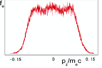
Figure 1: Electron distribution function $f_{e}(p_{z})$ (arb. units) formed as a result of optical field ionization of the gas target by a $40\,fs$ laser pulse with dimensionless amplitude $eE/m_{e}\omega_{0}c=0.1$, which is the tunneling regime of $\gamma_{K}\ll 1$ KCP . The $f_{e}$ dependence is on the normalised electron momentum $p_{z}/m_{e}c$ along the laser polarization direction.

II.2 Basic equations

Following Ref. RCD , we consider the electron phase space $(x,p)$ shown in Fig. 2, which corresponds to the support of the electron distribution function $f_{e}(p,x,t)$.

The electron distribution function is constant

$$f_{e}(p,x,t)={\rm constant}$$ (1)

within the region with borders marked by $p_{+}(x,t)$ and $p_{-}(x,t)$, while $f_{e}(p,x,t)=0$ outside this region. Here the constant is proportional to the ratio of the electron density and the momentum width. The electron distribution function can also be expressed via the unit step Heaviside functions:

$$f_{e}(p,x,t)={\rm constant}\times\theta(p-p_{-}(x,t))\,\theta(p_{+}(x,t)-p),$$ (2)

where $\theta(x)=0$ for $x<1$ and $\theta(x)=1$ for $x>1$.

The evolution of the distribution function is described by the Vlasov-Poisson system of equations

$$\partial_{t}f_{e}+v\partial_{x}f_{e}-E\,\partial_{p}f_{e}=0,$$ (3)

$$\partial_{x}E=1-n_{e},$$ (4)

where all the variables are written in a dimensionless form normalised in a standard way in which the time and space units are $\omega_{pe}^{-1}$ and $c\omega_{pe}^{-1}$, the momentum and the velocity are normalised on $m_{e}c$ and $c$, the unit for the electric field, $E(x,t)$, is $m_{e}\omega_{pe}c/e$, with $\omega_{pe}=(4\pi n_{0}e^{2}/m_{e})^{1/2}$ being the Langmuir frequency, $e$ and $m_{e}$ are the electron charge and mass, and $n_{0}$ is the density of ions which are assumed to be at rest. The electron velocity is equal to $v=p/(1+p^{2})^{1/2}$ , and $n_{e}(x,t)$ is the electron density normalised on $n_{0}$. Global charge neutrality is assumed. Eq. (3) describes the incompressible motion of the distribution $f_{e}$ in phase space.

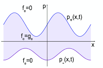
Figure 2: Electron phase space in a single water-bag model. The electron distribution function is constant $f_{e}(p,x,t)=g_{e}$ within the region with borders marked by $p_{+}(x,t)$ and $p_{-}(x,t)$, while $f_{e}(p,x,t)=0$ outside this region.

Calculating the first momentum of the distribution function we find that the electron density is related to the bounding curves $p_{+}(x,t)$ and $p_{-}(x,t)$ as

$$n_{e}(x,t)=\int\limits_{-\infty}^{+\infty}f_{e}(p,x,t)d{\rm p}=g_{e}\,[p_{+}(x,t)-p_{-}(x,t)],$$ (5)

where $g_{e}$ is a numerical constant (see Eq.(1)) that gives the ratio between the dimensionless electron density $n_{e}(x,t)$ and the dimensionless momentum width $\Delta p(x,t)\equiv p_{+}(x,t)-p_{-}(x,t)$, and is determined by the value of this ratio at $t=0$.

From Eqs. (3) and (4) it follows that the functions $p_{+}(x,t)$, $p_{-}(x,t)$ and $E(x,t)$ evolve according to (see also Ref.RCD )

$$\partial_{t}p_{+}+\frac{p_{+}}{\sqrt{1+p_{+}^{2}}}\partial_{x}p_{+}=-E,$$ (6)

$$\partial_{t}p_{-}+\frac{p_{-}}{\sqrt{1+p_{-}^{2}}}\partial_{x}p_{-}=-E,$$ (7)

$$\partial_{x}E=1-g_{e}(p_{+}-p_{-}).$$ (8)

II.3 Dispersion equation for the wave frequency and wave number

A large energy spread of the electron distribution function leads to a change of the Langmuir wave frequency due to its dependence on the plasma temperature. Linearization of Eqs. (6 – 8) around the equilibrium solution $p_{+}=p_{+,0}$, $p_{-}=p_{-,0}$, $E=0$ with $p_{-,0}=-p_{+,0}=\Delta p_{0}/2$ gives the dispersion equation for the frequency, $\omega$, and the wave-number $k$ in the case of the small amplitude Langmuir wave. In dimensional form it can be written as

$$\omega^{2}=\frac{8\pi n_{0}e^{2}c}{\sqrt{4m_{e}^{2}c^{2}+\Delta p_{0}^{2}}}+\frac{k^{2}c^{2}\Delta p_{0}^{2}}{4m_{e}^{2}c^{2}+\Delta p_{0}^{2}}.$$ (9)

The corresponding kinetic dispersion relation for a relativistic Maxwellian distribution function (Jüttner-Synge distribution) and its derivation in terms of relativistic fluid-like equations are given in Ref. PORPEG and references quoted therein. In particular waves with phase velocities larger than the speed of light are considered in Ref. PORPEG since in the case of the Jüttner-Synge distribution, and in general of a distribution that is not piece-wise constant in momentum space, waves with phase velocity smaller that the speed of light are heavily damped in the relativistic regime buti . It is shown that for these “superluminal” waves the relativistic electron population obeys an effective isothermal equation of state as soon as the normalized thermal momentum $p_{th}$ becomes larger than an appropriately redefined phase momentum $p_{ph}\equiv\omega/(\omega^{2}-k^{2}c^{2})^{1/2}$. We note that although the superluminal regime could also be considered within the water-bag formalism by redefining $\gamma_{ph}$ below Eq.(22), such a regime is not of interest for the investigation of wavebreaking. In fact, both Landau damping and wavebreaking are related to particles that have an unperturbed velocity (in the case of the linear Landau damping), or are accelerated by the wave electric field to a velocity that matches the wave phase velocity and this cannot occur for superluminal waves. Conversely, this indicates that thermal effects tend to favour Landau damping in the case of a particle distribution that is not piece-wise constant and wavebreaking in the case of a water-bag distribution.

As can be seen from Eq.(9) a finite temperature modifies the Langmuir frequency and makes it depend on the wavenumber, $k$. In terms of the variable $X=x-v_{ph}t$ the wave is characterised by the wavenumber $k_{w}$, which is given in dimensionless form by

$$k_{w}=\sqrt{\frac{\gamma_{+,0}}{\beta_{\rm ph}^{2}\gamma_{+,0}^{2}-p_{+,0}^{2}}},$$ (10)

where $\gamma_{+,0}=\sqrt{1+p_{0}^{2}}$. The wave number $k_{w}$ tends to infinity for $p_{+,0}/\gamma_{+,0}\to\beta_{\rm ph}$ . The frequency dependence on the electron temperature leads to a shortening of the wakewave wavelength. It results in a lower electric field in the wakewave in comparison to the case with a relatively small thermal spread.

II.4 Long wavelength limit

It is easy to obtain from Eqs. (6 – 8) that spatially homogeneous nonlinear oscillations of electrons in relativistic thermal plasmas are described by the system of ordinary differential equations

$$\frac{dp_{+}}{dt}=-E,$$ (11)

$$\frac{dE}{dt}=\frac{\sqrt{1+p_{+}^{2}}-\sqrt{1+(p_{+}-\Delta p_{0})^{2}}}{\Delta p_{0}},$$ (12)

where $\Delta p_{0}=p_{+,0}-p_{-,0}$. The Hamilton function corresponding to these equations is

$${\cal H}(E,p_{+})=\frac{E^{2}}{2}+{\Pi}(p_{+})$$ (13)

with the potential function

$${\Pi}(p_{+})=\frac{U(p_{+})-U(p_{+}-\Delta p_{0})}{2\Delta p_{0}},$$ (14)

where the function $U(z)$ is given by

$$U(z)=z\sqrt{1+z^{2}}+\ln{\left(z+\sqrt{1+z^{2}}\right)}.$$ (15)

Isocontours of the Hamiltonian function (13) in the plane $E,p_{+}$ are shown in Fig. 3a for $\Delta p_{0}=3$. The potential function ${\Pi}(p_{+})$ is plotted in Fig. 3b. Nonlinear oscillations are shown in Fig. 3c, where the time dependence of the electron momentum, $p_{+}(t)$ and electric field, $E(t)$ are plotted for $p_{+,0}=12.5$ and $\Delta p_{0}=7.5$. The momentum $p_{+}$ oscillates between the value $p_{+,0}$ and $-(p_{+,0}-\Delta p_{0})$.

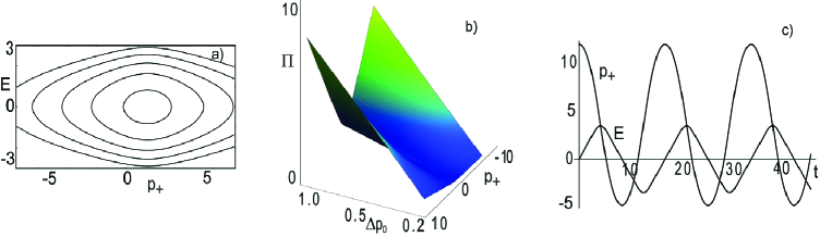
Figure 3: a) Isocontours of the Hamiltonian function (13) in the plane $(E,p_{+})$ for $\Delta p_{0}=3$; b) Potential function ${\Pi}(p_{+};\Delta p_{0})$; c) Time dependence of the electron momentum, $p_{+}(t)$ and electric field, $E(t)$, for $p_{+,0}=12.5$ and $\Delta p_{0}=7.5$.

In the small amplitude limit the oscillation frequency is given by expression (9) for $k=0$, i.e. $\omega=\frac{\left({8\pi n_{0}e^{2}c}\right)^{1/2}}{{\left(4m_{e}^{2}c^{2}+\Delta p_{0}^{2}\right)^{1/4}}}$. If the oscillation amplitude, $p_{\rm m}$, is large compared to the half-width of the distribution function, $\Delta p_{0}/2$, and $p_{\rm m}\gg 1$ then the oscillation period is given by $T=(4p_{\rm m}/\pi n_{0}e^{2})^{1/2}$ (see Ref. AP ).

II.5 Langmuir waves travelling with constant velocity

We consider waves propagating along the $x$ axis with constant phase velocity $v_{ph}$, where all functions depend on the independent variable

$$X=x-\beta_{\rm ph}t.$$ (16)

In this case Eqs. (6 – 8) take the form

$$h_{+}^{\prime}=-E,$$ (17)

$$h_{-}^{\prime}=-E,$$ (18)

and

$$E^{\prime}=1-\frac{p_{+}(h_{+})-p_{-}(h_{-})}{\Delta p_{0}},$$ (19)

where we introduced the dependent variables $h_{+}$ and $h_{-}$ defined by

$$h_{\pm}(p_{\pm})=\sqrt{1+p_{\pm}^{2}}-\beta_{\rm ph}p_{\pm},$$ (20)

a ”prime” denotes differentiation with respect to $X$ and $\beta_{\rm ph}=v_{ph}/c$. We use

$$\Delta p_{0}=p_{+,0}-p_{-,0},$$ (21)

with $p_{+,0}=p_{+}(X_{0})$ and $p_{-,0}=p_{-}(X_{0})$ taken at $X=X_{0}$, where $E^{\prime}=0$. Inverting Eq. (20) we obtain

$$p_{\pm}(h_{\pm})=\gamma_{\rm ph}^{2}\beta_{\rm ph}h_{\pm}-\sqrt{\gamma_{\rm ph}^{4}h_{\pm}^{2}-\gamma_{\rm ph}^{2}},$$ (22)

with $\gamma_{\rm ph}=1/\sqrt{1-\beta_{\rm ph}^{2}}$.

Here and below we assume ”subluminal” propagation velocity, i.e. $\beta_{\rm ph}\leq 1$.

II.6 Hamiltonian form of the equations describing a travelling Langmuir wave

Multiplying Eq. (19) by $E$ and using Eqs. (17) and (18) and integrating it over $X$, we obtain the integral

$${\frac{E^{2}}{2}+\frac{h_{+}}{2}\left(1-\frac{\gamma_{\rm ph}^{2}\beta_{\rm ph}h_{+}}{\Delta p_{0}}\right)+\frac{h_{-}}{2}\left(1+\frac{\gamma_{\rm ph}^{2}\beta_{\rm ph}h_{-}}{\Delta p_{0}}\right)}+\displaystyle{\frac{W(\gamma_{\rm ph}h_{+})-W(\gamma_{\rm ph}h_{-})}{2\Delta p_{0}}={\rm constant}},$$ (23)

where

$$W(z)=z\sqrt{z^{2}-1}\,-\,\ln{\left(z+\sqrt{z^{2}-1}\right)}.$$ (24)

This function vanishes at $z=1$. In the limit $z\to 1+0$ its behaviour is described as

$$W(z)=\frac{4}{3}\sqrt{2}(z-1)^{3/2}+O(z-1)^{5/2}.$$ (25)

For $z\to\infty$ we have

$$W(z)=z^{2}-\frac{1}{2}-\ln{2z}+\frac{1}{8z^{2}}+O\left(\frac{1}{z^{3}}\right).$$ (26)

According to Eqs. (17) and (18) the variables $h_{-}$ and $h_{+}$, are not independent and are related by

$$h_{-}=h_{+}-\Delta h_{0},$$ (27)

where the constant $\Delta h_{0}$ is determined by the values of $p_{+}$ and $p_{-}$ at $X=X_{0}$:

$${\Delta h_{0}=h_{+,0}-h_{-,0}}\displaystyle{\equiv\sqrt{1+p_{+,0}^{2}}-\sqrt{1+p_{-,0}^{2}}-\beta_{\rm ph}(p_{+,0}-p_{-,0})}.$$ (28)

As a result, Eqs. (17, 18) and (19) can be rewritten in the form

$$h_{+}^{\prime}=-E,$$ (29)

$$E^{\prime}=1-\frac{p_{+}(h_{+})-p_{-}(h_{+}-\Delta h_{0})}{\Delta p_{0}}.$$ (30)

This is a Hamiltonian system with Hamilton function

$${\cal H}(E,h_{+})=\displaystyle{\frac{E^{2}}{2}+\Pi(h_{+})},$$ (31)

where $h_{+}$ and $-E$ are canonical variables, and

$$\Pi(h_{+})=\displaystyle{h_{+}\left(1-\frac{\gamma_{\rm ph}^{2}\beta_{\rm ph}\Delta h_{0}}{\Delta p_{0}}\right)}\displaystyle{+\,\frac{W(\gamma_{\rm ph}h_{+})-W(\gamma_{\rm ph}(h_{+}-\Delta h_{0}))}{2\Delta p_{0}}}.$$ (32)

For a symmetrical distribution where $p_{+,0}=-p_{-,0}$ Eq. (28) takes the simpler form $\Delta h_{0}=-\beta_{\rm ph}\Delta p_{0}$ and the potential $\Pi(h_{+})$ reduces to

$$\Pi_{\rm sym}(h_{+})=\displaystyle{\gamma_{\rm ph}^{2}h_{+}}\displaystyle{+\,\frac{W(\gamma_{\rm ph}h_{+})-W(\gamma_{\rm ph}(h_{+}+\beta_{\rm ph}\Delta p_{0}))}{2\Delta p_{0}}}.$$ (33)

The potential $\Pi(h_{+})$ is plotted in Fig. 4a as a function of $h_{+}$, $\beta_{\rm ph}$ for four values of $\Delta p_{0}$ assuming that $p_{+,0}=-p_{-,0}$, i.e. $\Delta h_{0}=-\beta_{\rm ph}\Delta p_{0}$. Isocontours of the Hamiltonian function in the plane $E,h_{+}$ for $\beta_{\rm ph}=0.8$ and $\Delta p_{0}=0.1$ are shown in Fig. 4b.

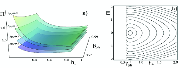
Figure 4: a) Potential function $\Pi(h_{+})$ vs $h_{+}$ and $\beta_{\rm ph}$ for $\Delta p_{0}=0.01,0.1,0.3,0.5$; b) Isocontours of the Hamiltonian function in the plane $(E,h_{+})$ for $\beta_{\rm ph}=0.8$ and $\Delta p_{0}=0.1$.

III The wavebreaking limits

III.1 Crested Langmuir wave

The system of Eqs. (17-19) has a singular solution when $h_{+}\to\gamma_{\rm ph}^{-1}$, i.e.

$$p_{+}\to p_{+,{\rm br}}=\frac{\beta_{\rm ph}}{\sqrt{1-\beta_{\rm ph}^{2}}},$$ (34)

which corresponds to the wavebreak in thermal plasmas when the electron velocity calculated for the momentum on the upper bound curve, $p_{+}(x,t)$, becomes equal to the wave phase velocity. In this limit $dh_{+}/dp_{+}\to 0$ and the upper bound curve is no longer a single valued function of $X$.

The electron momentum on the lower bound curve at wavebreak is

$$p_{-,br}=p_{+,{\rm br}}-\beta_{\rm ph}\gamma_{\rm ph}^{2}\Delta h_{0}-\sqrt{\gamma_{\rm ph}^{4}\Delta h_{0}^{2}-2\gamma_{\rm ph}^{3}\Delta h_{0}}.$$ (35)

Eqs. (5, 34, 35) give for the electron density at the wavebreaking point

$$n_{e,{\rm br}}=\displaystyle{\frac{\sqrt{\gamma_{\rm ph}^{4}\Delta h_{0}^{2}-2\gamma_{\rm ph}^{3}\Delta h_{0}}+\beta_{\rm ph}\gamma_{\rm ph}^{2}\Delta h_{0}}{\Delta p_{0}}}.$$ (36)

For a symmetric distribution function such that $p_{+,0}=-p_{-,0}$ from the electron density dependence on $h$,

$$n_{e}(h)=\frac{\gamma_{\rm ph}\displaystyle{\left[\sqrt{\gamma_{\rm ph}^{2}(h+\beta_{\rm ph}\Delta p_{0})^{2}-1}-\sqrt{\gamma_{\rm ph}^{2}h^{2}-1}\right]}}{\Delta p_{0}}-\gamma_{\rm ph}^{2}\beta_{\rm ph}^{2},$$ (37)

it follows that at the wavebreaking point, $h\to\gamma_{\rm ph}^{-1}$, the density tends to

$$n_{e,{\rm br}}=\gamma_{\rm ph}^{2}\beta_{\rm ph}\left(\sqrt{1+\frac{2}{\beta_{\rm ph}\gamma_{\rm ph}\Delta p_{0}}}-\beta_{\rm ph}\right).$$ (38)

In the nonrelativistic limit, when $\beta_{\rm ph}\ll 1$, $\Delta p_{0}\ll 1/\beta_{\rm ph}$, and $\gamma_{\rm ph}\approx 1$, the density is

$$n_{e,{\rm br}}\approx\sqrt{\frac{2\beta_{\rm ph}}{\Delta p_{0}}}-\gamma_{\rm ph}^{2}\beta_{\rm ph}^{2}.$$ (39)

In the ultrarelativistic limit, when $\beta_{\rm ph}\approx 1$, and $\gamma_{\rm ph}\gg 1$ we have

$$n_{e,{\rm br}}\approx\sqrt{\frac{2\beta_{\rm ph}\gamma_{\rm ph}^{3}}{\Delta p_{0}}}-\gamma_{\rm ph}^{2}\beta_{\rm ph}^{2}$$ (40)

provided $\Delta p_{0}\ll{2}/\beta_{\rm ph}\gamma_{\rm ph}$ (see also SMF ) while for $\Delta p_{0}=2\beta_{\rm ph}\gamma_{\rm ph}$ we have $n_{e,{\rm br}}=1$, because in this limit a wave with arbitrarily small amplitude breaks, as seen from Eq. (10). In the above considered cases the electron density written in dimensional units is

$$n_{e,{\rm br}}\approx n_{0}\sqrt{\frac{m_{e}v_{\rm ph}}{p_{+,0}}}$$ (41)

for a nonrelativistic plasma wave and

$$n_{e,{\rm br}}\approx n_{0}\sqrt{\frac{m_{e}c\beta_{\rm ph}\gamma_{\rm ph}^{3}}{p_{+,0}}}$$ (42)

in the limit $\gamma_{\rm ph}\gg 1$.

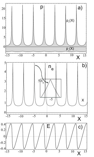
Figure 5: Structure of the nonlinear wake wave: a) electron phase space, b) the electron density (in the inset the density distribution is shown in the vicinity of the maximum), c) electric field as functions of the coordinate $X$. The normalised wave phase velocity is $\beta_{\rm ph}=0.999$; the plasma thermal momentum width at $X=15$ is $\Delta p_{0}=p_{+,0}-p_{-,0}=5$; the maximum of the electric field is $E_{\rm m}=0.4190625$.

In order to find the density behaviour in the neighbourhood of the breaking point, we expand the electron momentum, $p_{+}$, on the upper bound curve, in the vicinity of its maximum, $\delta X=X-X_{\rm br}\to 0$. Here $X_{\rm br}$ is the location of the breaking point. Locally, the momentum is represented by

$$p_{+}=p_{+,{\rm br}}-\delta p_{+}+O(\delta p_{+}^{2})$$ (43)

with $p_{+,{\rm br}}$ given by Eq. (34). Keeping the main terms of the expansion over $\delta p_{+}$ of Eq. (37) we obtain for the electron density

$$n_{e}=n_{e,{\rm br}}-\frac{\delta p_{+}}{\Delta p_{0}},$$ (44)

where we used the expression $h\approx\gamma_{\rm ph}^{-1}+\delta p_{+}^{2}/2\gamma_{\rm ph}^{3}$. From Eqs. (29, 30) for the dependence of $\delta p_{+}$ on $X$ we have

$$(\delta p_{+}^{2})^{\prime\prime}=2n_{e,{\rm br}}\gamma_{\rm ph}^{3}.$$ (45)

Integrating this expression we find

$$\delta p_{+}=\pm\sqrt{n_{e,{\rm br}}\gamma_{\rm ph}^{3}}\delta X,$$ (46)

where we assumed that $\delta p_{+}^{\prime}$ at $\delta X$ vanishes, i.e. the electric field at the breaking point is equal to zero. Since by assumption $\delta p_{+}$ must be non-negative, we must chose the $"-"$ sign in the interval $\delta X<0$ and the $"+"$ sign for $\delta X>0$. As a result we can write for the momentum $p_{+}$ in the vicinity of the wavebreaking point

$$p_{+}\sim p_{+,{\rm br}}-\sqrt{n_{e,{\rm br}}\gamma_{\rm ph}^{3}}|\delta X|.$$ (47)

From the expression (5) for the density, and recalling that at wavebreak $\delta p_{-}\propto(\delta p_{+})^{2}$, we find that in the vicinity of the breaking point the electron density can be written as (see also SMF )

$$n_{e}\sim{n_{e,{\rm br}}}-\frac{\sqrt{n_{e,{\rm br}}\gamma_{\rm ph}^{3}}}{\Delta p_{0}}\,|\delta X|.$$ (48)

This type of wave breaking in the general case corresponds to the ”peakon” structures known in water waves Stokes ; Whitham ; peakon . It can also be called ”$\Lambda$-type” breaking.

The structure of the nonlinear wake wave of the electron density, the electron phase space and the electric field is shown in Fig. 5, as obtained by numerical integration of Eqs. (6 – 8). In Fig. 5 we show the high temperature case with the initial distribution function width $p_{+,0}$ comparable with the value of electron momentum on the upper bound curve at the wavebreaking point, $p_{\rm br}$. From Fig. 5b we see that in the vicinity of the density maximum (see inset to Fig. 5b), the density dependence on $X$ corresponds to Eq. (48).

III.2 Maximum electric field in stationary wave

As is seen from the trajectory pattern in the $E,h_{+}$ plane presented in Fig. 4b, the electric field maximum is reached at the point $h_{+}=h_{E}$ (see also Fig. 6) where the derivative of the electric field with respect to $h_{+}$ vanishes, $\left.dE/dh_{+}\right|_{h_{+}=h_{E}}=0$. This condition results in the equation for $h_{E}$:

$$\Delta p_{0}=p_{+}(h_{E})-p_{+}(h_{E}+\beta_{\rm ph}\Delta p_{0}),$$ (49)

where the function $p_{+}(h_{E})$ is given by Eq. (22). Here we assume the symmetric distribution with $p_{+,0}=-p_{-,0}=\Delta p_{0}/2$. The solution of Eq. (49) is

$$h_{E}=\sqrt{1+\frac{\Delta p_{0}^{2}}{4}}-\frac{\beta_{\rm ph}\Delta p_{0}}{2}.$$ (50)

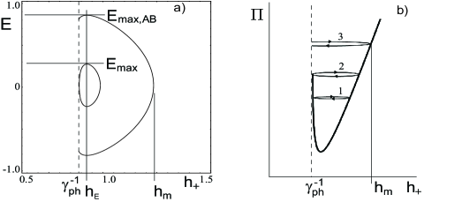
Figure 6: a) Isocontours of the Hamiltonian function ($H_{1}=1.9125$ and $2.25$) in the plane $(E,h_{+})$ for $\beta_{\rm ph}=0.6$ and $\Delta p_{0}=0.05$. The electric field maxima $E_{\max}$ and $E_{\rm max,AB}$ are reached at $h_{+}=h_{E}$. b) The curves $1,2,3$ indicate the potential $\Pi(h)$ values corresponding to (1) a periodic wave with amplitude below the wave breaking limit, (2) to a wave at the wave breaking threshold, and (3) to a wave with amplitude above the wave breaking limit. Vertical dashed line marks the wave breaking boundary.

The last bound trajectory in the $E,h_{+}$ plane is determined by the equation

$$\frac{E^{2}}{2}+\Pi(h_{+})=\Pi(\gamma_{\rm ph}^{-1})$$ (51)

with the potential given by Eq. (33). Substituting $h_{+}=h_{E}$ we find the electric field maximum

$$E_{\max}=\sqrt{2\left[\Pi(\gamma_{\rm ph}^{-1})-\Pi(h_{E})\right]}.$$ (52)

In the limit of cold plasma, when $\Delta p_{0}\to 0$, i.e. $p_{\pm}\to p$ with $p_{\pm,0}\to 0$ the Hamilton function (31) reduces to

$${\cal H}(E,h)=\displaystyle{\frac{E^{2}}{2}+\gamma_{\rm ph}^{2}h-\beta_{\rm ph}\sqrt{h^{2}\gamma_{\rm ph}^{4}-\gamma_{\rm ph}^{2}}},$$ (53)

where $h=\sqrt{1+p^{2}}-\beta_{\rm ph}p$. It can be rewritten in the form of the energy integral, $E^{2}/2+\gamma={\rm constant}$.

The potential $\Pi(h)=\gamma_{\rm ph}^{2}h-\beta_{\rm ph}\sqrt{h^{2}\gamma_{\rm ph}^{4}-\gamma_{\rm ph}^{2}}$ is plotted in Fig. 7a as a function of $h$ and $\beta_{\rm ph}$. Isocontours of the Hamiltonian function in the plane $E,h$ for $\beta_{\rm ph}=0.5$ are shown in Fig. 7b.

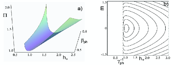
Figure 7: a) Potential function $\Pi(h)$ vs $h$; b) Isocontours of the Hamiltonian function in the plane $(E,h)$ for $\beta_{\rm ph}=0.5$.

It is easy to see that the electric field equals zero at the maximum of the electron quiver energy. This condition yields the result obtained in Ref. AP for the maximum value of the electric field:

$$E_{\rm AP}=\sqrt{2(\gamma_{\rm ph}-1)}.$$ (54)

For small but finite electron temperature, $\Delta p_{0}\ll 1/(\beta_{\rm ph}\gamma_{\rm ph})$, we obtain (see also Ref. ESL2 )

$$E_{\max}\approx\sqrt{2(\gamma_{\rm ph}-1)}-\frac{2}{3}\frac{(\beta_{\rm ph}\gamma_{\rm ph})^{3/2}}{\sqrt{(\gamma_{\rm ph}-1)}}\sqrt{\Delta p_{0}}.$$ (55)

At $\Delta p_{0}\to 2\beta_{\rm ph}\gamma_{\rm ph}$ the electric field vanishes because, as mentioned before, in this limit the wave with arbitrarily small amplitude breaks.

In Fig. 8 we show the maximum electric field, $E_{\max}$, in the breaking wake wave. The dependence of this field, normalized on $E_{\rm AP}$, on the wave phase velocity $\beta_{\rm ph}$ and on the width of the electron distribution function $\Delta p_{0}$ is presented in Fig. 8 a. Figures 8 b and c show dependences of $E_{\max}$ and $E_{\rm AP}$ on $\gamma_{\rm ph}$ for small and large $\Delta p_{0}$. We see that in the limit $\gamma_{\rm ph}\gg 1$ the difference between $E_{\max}$ and $E_{\rm AP}$ increases according to Eq. (55). Figures 8 a and c clearly illustrate the above mentioned fact that in the limit $\Delta p_{0}\to 2\beta_{\rm ph}\gamma_{\rm ph}$ the value of $E_{\rm max}$ vanishes.

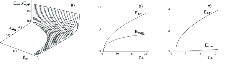
Figure 8: Maximum electric field in the breaking wake wave: a)$E_{\max}$ normalized on $E_{\rm AP}$, depending on the wave phase velocity $\beta_{\rm ph}$ and the width of the electron distribution function, $\Delta p_{0}$; The curve in the $\beta_{\rm ph}$ - $\Delta p_{0}$ plane where $E_{\max}=0$ is given by $\Delta p_{0}=2\beta_{\rm ph}\gamma_{\rm ph}$. b) $E_{\max}$ and $E_{\rm AP}$ v.s. $\gamma_{\rm ph}$ for $\Delta p_{0}=0.125$. c) $E_{\max}$ and $E_{\rm AP}$ v.s. $\gamma_{\rm ph}$ for $\Delta p_{0}=7.5$.

Independently of whether the plasma temperature is finite or vanishes, from Eqs. (31) and (53) we obtain that the second derivative of the potential $\Pi$ with respect to $h_{+}$ ($h$) becomes singular at $h_{+}=\gamma_{\rm ph}^{-1}$ ($h=\gamma_{\rm ph}^{-1}$), which corresponds to the vertical (dashed) singular line in Figs. 3b and 6b. In this limit the Hamiltonian in Eq. (53) takes the value

$$\frac{E^{2}}{2}+\gamma_{\rm ph},\quad{\rm while}\quad\gamma(h=\gamma_{\rm ph}^{-1})=\gamma_{\rm ph}.$$ (56)

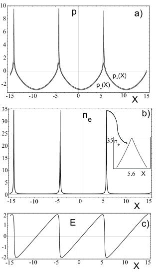
Figure 9: Structure of nonlinear wake wave: a) electron phase space, b) the electron density (in the inset the density distribution is shown in the vicinity of the maximum), c) electric field as functions of the coordinate $X$. The normalised wave phase velocity is $\beta_{\rm ph}=0.995$; the plasma thermal momentum width at $X=15$ is $\Delta p_{0}=p_{+,0}-p_{-,0}=0.25$; the maximum of the electric field is $E_{m}=1.9876$.

III.3 Cold wavebreaking limit

In order to compare the properties of the singularities formed in thermal and cold plasmas we reproduce here the dependence of the electron momentum and density on the coordinates in the cold wavebreaking case (for details see Ref. PAN ). In the cold plasma with $p_{+,0}\to 0$ and $p_{-,0}\to 0$, which implies $p_{+}(X)=p_{-}(X)\equiv p$, equations (17 – 19) can be reduced to

$$\left(\sqrt{1+p^{2}}-\beta_{\rm ph}p\right)^{\prime\prime}=\frac{p}{\beta_{\rm ph}\sqrt{1+p^{2}}-p}.$$ (57)

The solution of this equation can be expressed in terms of elliptic integrals. In order to analyze these solutions in the vicinity of the singularity we note that its right-hand side becomes singular when the denominator, $\beta_{\rm ph}\sqrt{1+p^{2}}-p$, tends to zero, i.e., when the electron velocity $v$ becomes equal to the phase velocity of the wake wave. In the wake wave, the singularity is reached at the maximum value of the electron momentum, $p_{\rm m}=p_{\rm br}$. We assume that the singularity is located at the coordinate $X=X_{\rm br}$. We consider the wave structure in the vicinity of the singularity, and find that here the electron momentum depends on $\delta X=X-X_{\rm br}$ as

$$p=p_{\rm br}-\beta_{\rm ph}^{1/3}\gamma_{\rm ph}^{2}(3|\delta X|/2^{1/2})^{2/3}.$$ (58)

The electron density tends to infinity as

$$n\approx n_{0}\gamma_{\rm ph}(2^{1/2}\beta_{\rm ph}/3|\delta X|)^{-2/3}.$$ (59)

The $2/3$ power behaviour can be recognized in Fig. 9, which presents the wakewave generated in a relatively low temperature plasma with $p_{+,0}\ll p_{\rm br}$. However, from Fig. 9b we see that in the very vicinity of the density maximum (see inset to Fig. 9b), the dependence of the electron density and momentum on $X$ still corresponds to Eq. (48), showing at the wave crest the density profile which can be approximated by the ”peakon” dependence. The electron distribution width, $p_{\rm{+,br}}-p_{\rm{-,br}}$, near the maximum is characterized by the value

$$\Delta p=p_{\rm{+,br}}-p_{\rm{-,br}}\approx\sqrt{2\beta_{\rm ph}\gamma_{\rm ph}^{3}\Delta p_{0}},$$ (60)

where we assumed $\gamma_{\rm ph}\Delta p_{0}\ll 1$.

IV Hydrodynamic approach

IV.1 Waterbag distribution

The system of Eqs. (6 –8) can be written as a system of hydrodynamic-type equations

$$\partial_{t}{\mathbb{N}}+\partial_{x}{\mathbb{J}}=0,$$ (61)

$$\partial_{t}{\mathbb{P}}+\partial_{x}{\mathbb{G}}=-E,$$ (62)

$$\partial_{t}E+{\mathbb{V}}\partial_{x}E={\mathbb{V}}$$ (63)

for the electron density

$${\mathbb{N}}(x,t)=\int{f_{e}(p,x,t)dp}=\frac{1}{\Delta p_{0}}(p_{+}-p_{-}),$$ (64)

average momentum

$${\mathbb{P}}(x,t)=\frac{1}{{\mathbb{N}}}\int{pf_{e}(p,x,t)dp}=\frac{p_{+}^{2}-p_{-}^{2}}{2(p_{+}-p_{-})}=\frac{1}{2}(p_{+}+p_{-}),$$ (65)

and electric field $E$. Here

$${\mathbb{J}}(x,t)=\int{\frac{p}{\sqrt{1+p^{2}}}f_{e}(p,x,t)dp}=\frac{1}{\Delta p_{0}}(\gamma_{+}-\gamma_{-}),$$ (66)

with $\gamma_{\pm}={\sqrt{1+p_{\pm}^{2}}}$,

$${\mathbb{V}}(x,t)=\frac{1}{\mathbb{N}}\int{\frac{p}{\sqrt{1+p^{2}}}f_{e}(p,x,t)dp}=\frac{p_{+}+p_{-}}{\gamma_{+}+\gamma_{-}},$$ (67)

and

$${\mathbb{G}}(x,t)=\frac{\displaystyle{\int{pf_{e}(p,x,t)dp}}}{\displaystyle{\int{\frac{p}{\sqrt{1+p^{2}}}f_{e}(p,x,t)dp}}}=\frac{1}{2}(\gamma_{+}+\gamma_{-}),$$ (68)

These functions are related to each other as

$${\mathbb{V}}=\frac{{\mathbb{P}}}{\mathbb{G}}=\frac{{\mathbb{J}}}{\mathbb{N}}$$ (69)

and

$${\mathbb{G}}=\sqrt{\frac{1}{4}+\left(\frac{{\mathbb{P}}}{2}+\frac{{\mathbb{N}}\Delta p_{0}}{4}\right)^{2}}+\sqrt{\frac{1}{4}+\left(\frac{{\mathbb{P}}}{2}-\frac{{\mathbb{N}}\Delta p_{0}}{4}\right)^{2}}.$$ (70)

In the case of a wave travelling with constant velocity $c\beta_{\rm ph}$, the functions ${\mathbb{N}},{\mathbb{P}},{\mathbb{G}}$ and $E$ depend on the variable $X=x-\beta_{\rm ph}t$ and Eqs. (61 – 63) can be reduced to

$$\left({\mathbb{G}}-\beta_{\rm ph}{\mathbb{P}}\right)^{\prime\prime}=-\frac{{\mathbb{P}}}{\beta_{\rm ph}{\mathbb{G}}-{\mathbb{P}}},$$ (71)

$${\mathbb{N}}=\frac{\beta_{\rm ph}{\mathbb{G}}}{\beta_{\rm ph}{\mathbb{G}}-{\mathbb{P}}},$$ (72)

where a prime denotes differentiation with respect to $X$. Equation (71) looks identical to Eq. (57) which describes the wave break at $p/\gamma\to\beta_{\rm ph}$ and the formation of a singularity in the electron density, $n\to\infty$, according to Eq. (59). However, due to the nonlinear dependence of ${\mathbb{G}}$ on ${\mathbb{P}}$ given by relationships (70) and (72) the character of the singularity changes and becomes of the type described in Sec. III.1. In particular, we can see that the condition for the denominator in the r.h.s. of Eq. (71) to vanish implies that ${\mathbb{V}}=\beta_{\rm ph}$. This condition can be rewritten as

$$\beta_{\rm ph}=\frac{p_{+}+p_{-}}{\gamma_{+}+\gamma_{-}}=\frac{p_{+}}{\gamma_{+}}\left(\frac{1+p_{-}/p_{+}}{1+\gamma_{-}/\gamma_{+}}\right).$$ (73)

Assuming that in this limit $p_{-}=p_{+}+\delta p$ with $\delta p/p_{+}\ll 1$, we can easily find that the condition of ”hydrodynamic type wave break”(73) used in KM is equivalent to

$$\beta_{\rm ph}=\frac{p_{+}+p_{-}}{\gamma_{+}+\gamma_{-}}=\frac{p_{+}}{\gamma_{+}}\left(1-\frac{\delta p}{p_{+}^{3}}\right),$$ (74)

which requires ${p_{+}}/{\gamma_{+}}>\beta_{\rm ph}$, i.e. the waterbag description in the adopted limit of a stationary nonlinear wave propagating with constant velocity is no longer valid.

IV.2 Nonrelativistic limit

In the nonrelativistic limit Eqs. (61) and (62) take the form (see Ref. RCD )

$$\partial_{t}{\mathbb{N}}+\partial_{x}\left({\mathbb{N}}{\mathbb{V}}\right)=0,$$ (75)

$$\partial_{t}{\mathbb{V}}+{\mathbb{V}}\partial_{x}{\mathbb{V}}=-E-\frac{\Delta p_{0}^{2}}{8}\partial_{x}{\mathbb{N}}^{2},$$ (76)

which corresponds to a gasdynamics system where the pressure depends on the gas density as

$$P=\frac{P_{0}}{{\mathbb{N}}_{0}^{3}}{\mathbb{N}}^{3}$$ (77)

with $P_{0}$=const.

For a wave travelling with constant velocity, $\beta_{\rm ph}$, we obtain

$$\left[\frac{1}{2}\left({\mathbb{V}}-\beta_{\rm ph}\right)^{2}-\frac{\beta_{\rm ph}^{2}\Delta p_{0}^{2}}{8\left({\mathbb{V}}-\beta_{\rm ph}\right)^{2}}\right]^{\prime\prime}=-\frac{{\mathbb{V}}}{\beta_{\rm ph}-{\mathbb{V}}}.$$ (78)

The singular points of this equation correspond to

$${\mathbb{V}}_{1}=\beta_{\rm ph}\quad{\rm and}\quad{\mathbb{V}}_{2,3}=\beta_{\rm ph}\pm\sqrt{\frac{\beta_{\rm ph}\Delta p_{0}}{2}}.$$ (79)

We see that the points ${\mathbb{V}}_{1}$ and ${\mathbb{V}}_{2}$ lay beyond the applicability range of the waterbag model, while a wave with ${\mathbb{V}}_{\max}\to{\mathbb{V}}_{3}$ is qualitatively described by Fig. 9 with maximum density $n_{\max}=\sqrt{2\beta_{\rm ph}/\Delta p_{0}}$ and electric field $E_{\max}\approx\beta_{\rm ph}-\sqrt{\beta_{\rm ph}\Delta p_{0}/2}$.

IV.3 Ultrarelativistic limit

This case corresponds to the limit ${\mathbb{P}}\gg 1$. Expanding Eq.(70) into series of the small parameter ${\mathbb{N}}\Delta p_{0}/{\mathbb{P}}\ll 1$ we obtain

$${\mathbb{G}}\approx\sqrt{1+{\mathbb{P}}^{2}}+\frac{{\mathbb{N}}^{2}\Delta p_{0}^{2}}{8(1+{\mathbb{P}}^{2})^{3/2}}.$$ (80)

Using Eq. (72) for the electron density ${\mathbb{N}}$ we find from Eqs. (71) and (80)

$$\left[\sqrt{1+{\mathbb{P}}^{2}}-\beta_{\rm ph}{\mathbb{P}}+\frac{\beta_{\rm ph}^{2}\Delta p_{0}^{2}}{8\sqrt{1+{\mathbb{P}}^{2}}(\beta_{\rm ph}\sqrt{1+{\mathbb{P}}^{2}}-{\mathbb{P}})^{2}}\right]^{\prime\prime}=-\frac{{\mathbb{P}}}{\beta_{\rm ph}\sqrt{1+{\mathbb{P}}^{2}}-{\mathbb{P}}}.$$ (81)

The singular points of this equation, written in terms of the average velocity ${\mathbb{V}}={\mathbb{P}}/\sqrt{1+{\mathbb{P}}^{2}}$, are given by

$${\mathbb{V}}_{1}\approx\beta_{\rm ph}\quad{\rm and}\quad{\mathbb{V}}_{2,3}\approx\beta_{\rm ph}\pm\sqrt{\frac{\beta_{\rm ph}\Delta p_{0}}{2\gamma_{\rm ph}^{3}}}$$ (82)

with ${\mathbb{V}}_{3}$ corresponding to the wake wave breaking. This yields for maximum density $n_{\max}\approx\sqrt{2\beta_{\rm ph}\gamma_{\rm ph}^{3}/\Delta p_{0}}$ and for the electric field $E_{\max}\approx\sqrt{2(\gamma_{\rm ph}-1)}-(2/3)\gamma_{\rm ph}\sqrt{\beta_{\rm ph}\Delta p_{0}}$ in agreement with Eqs. (40) and (55).

V Computer simulation of the plasma wave breaking in thermal plasmas

During the irradiation of underdense plasma targets by high-power laser pulses, the light within the pulse generates a finite amplitude wake wave whose parameters depend, in particular, on the plasma temperature and on the interaction geometry. A thorough study of these effects require computer simulations. We performed parametric studies of the laser pulse interaction with underdense targets using a two-dimensional (2D3P) particle-in-cell (PIC) code NPIC .

Here the effects of the finite electron temperature have been taken into account in three limiting cases. In the first case the initial electron temperature has been assumed to be equal to zero. In the second case thermal effects have been modelled by the electron distribution corresponding to the initial waterbag distribution function with a temperature equal to $100$eV. In the third case, the initial electron distribution was Maxwellian with the same temperature. In both the cases of the waterbag and Maxwellian distributions, the total electron energy is the same, i.e., average energy for the waterbag case,

$$\left<m_{e}c^{2}(\gamma-1)\right>\approx\left<\frac{p^{2}}{2\,m_{e}}\right>=\displaystyle{\frac{\int_{0}^{\Delta p_{0}}(p^{2}/2\,m_{e})p^{2}dp}{\int_{0}^{\Delta p_{0}}p^{2}dp}=\frac{3\Delta p_{0}^{2}}{40m_{e}}},$$ (83)

is set to be equal to that in the case of a Maxwellian distribution, $<p^{2}/2\,m_{e}>=(3/2)k_{B}T$. Here we assumed that $p/mc\ll 1$.

In these simulations, the laser pulse has a normalized amplitude of $a_{0}=eE_{0}/m_{e}\omega c=4.6$, a wavelength of $\lambda=2\pi c/\omega=0.8\,\mu$m, focused onto a spot of the size of $13\mu$m, and duration of 16 fs. The plasma density equals $4\times 10^{19}$cm^-3. The width of the simulation box is equal to $50\times 65\lambda^{2}$. The mesh size is $\Delta x=\lambda/160$ with 30 particles per cell.

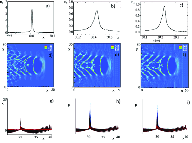
Figure 10: Results of 2D-PIC simulations of the nonlinear wake wave generation in thermal plasmas: electron density and phase space in a cold plasma (a,d,g); in the plasma described by the waterbag distribution with a temperature of 100 eV (b,e,h); in the plasma described by the Maxwellian distribution with a temperature of 100 eV (c,f,i).

Simulation results for the parameters of interest are shown in Fig. 10. Here the $x$ coordinate is measured in $1\,\mu$m, the electron momentum $p$ is normalized on $m_{e}c$, and the density is normalized on the critical density $n_{cr}=m_{e}\omega^{2}/4\pi e^{2}$. The figures are plotted for the time when the highest density is reached, which is 350 fs, 310fs, 310fs for zero-temperature, waterbag, and Maxwellian distribution, respectively. In the cold plasma case, the electron density distribution in the first maximum of the breaking wake wave takes a cusp-like form (see Fig. 10 a. In Figs. 10 b and c we see that the finite temperature effects lead to a decrease of the maximum electron density in the breaking wake wave, to the broadening of the maximum and to the formation of peakon-like structures for both the waterbag and the Maxwellian distributions. Note here more efficient electron injection in the finite temperature plasma compared with the cold plasma case.

VI Above the wavebreaking limit

VI.1 Maximal electric field

The limiting electric field given by Eq. (54) corresponds to a stationary Langmuir wave for which the electron quiver energy is below $m_{e}c^{2}\gamma_{\rm ph}$. When the Langmuir wave is excited by a short laser pulse its amplitude and its phase velocity depend on the plasma density and on the laser pulse intensity ESL1 . Propagating in an underdense plasma, an intense laser pulse can accelerate plasma electrons longitudinally up to the energy $m_{e}c^{2}(1+a^{2}/2)$. In a cold plasma the wavebreaking condition corresponds to $(1+a^{2}/2)=\gamma_{\rm ph}$, where $\gamma_{\rm ph}=(n_{cr}/n_{0})(1+a^{2})^{1/4}$ is the Lorentz gamma-factor calculated for the wake wave phase velocity which is equal to the laser pulse group velocity. Here the dependence of the electromagnetic wave group velocity on its amplitude is taken into account according to AP . This yields the wake wave breaking threshold in terms of the driver laser pulse amplitude EK

$$a>\left(4\frac{n_{cr}}{n_{0}}\right)^{1/3}.$$ (84)

In general, the laser pulse amplitude in a plasma is different from its value in vacuum due to the laser pulse self-focusing and self-channelling RSF . The laser pulse amplitude inside the self-focusing channel relates to the laser power ${\cal P}$ and plasma density as SSB

$$a_{0}^{3}>8\pi\frac{{\cal P}}{{\cal P}_{c}}\frac{n_{0}}{n_{cr}},$$ (85)

where ${\cal P}_{c}=2m_{e}^{2}c^{5}/e^{2}\approx 17$GW.

Using Eqs. (84) and (85) we obtain the wake wave breaking threshold:

$${\cal P}>\frac{{\cal P}_{c}}{2\pi}\left(\frac{n_{cr}}{n_{0}}\right)^{2}.$$ (86)

For example, from Eqs. (84) and (86) we find that if a laser pulse of the wavelength $\lambda=0.8\mu$m, for which $n_{cr}\approx 2\times 10^{21}{\rm cm}^{-3}$, propagates in a plasma with density $n_{0}=2\times 10^{19}{\rm cm}^{-3}$, the wavebreaking threshold is reached for ${\cal P}>30\,$TW and $a_{0}=7.3$, i.e. for a laser intensity of the order of $7\times 10^{19}\,{\rm W/cm}^{2}$.

A laser pulse with power larger than that given by the r.h.s of Eq. (86), causes the wake wave to break in the first period, with the electric field well above the limiting value given by Eq. (54) and with a number of electrons piled up in the singularity region much larger than in the stationary case described by Eqs. (36) and (59). This fact has important consequences for determining the laser wakefield acceleration scaling LWFA ; ESL1 .

A wakewave with an amplitude above the wave break threshold is transient and forms a region with multi-stream electron motion. The multi-stream motion region expands in the forward direction at a relative velocity $dX/dt\approx c(1-\beta_{\rm ph})\approx c/2\gamma^{2}_{ph}$. Since in the limit $\gamma_{\rm ph}\gg 1$ this velocity is low, the region with a large electric field (and with a large number of electrons) can exist for a substantially long time, which is of the order of the charged particle acceleration time, $t_{\rm acc}=2\lambda_{w}\gamma^{2}_{ph}/c$. Here $\lambda_{w}$ is the wake wave wavelength.

The structure of the wake wave both below and above the wavebreaking limit can be revealed from the phase plane pattern presented in Figs. 4 b and 7 b. The stationary (periodic) waves correspond to the bound trajectories in the phase plane shown in Figs. 4 b and 7 b. The stationary breaking wave is described by a last closed trajectory touching the vertical (dashed) singular line, corresponding to $h_{+}=\gamma_{\rm ph}^{-1}$, in this figure.

In the vicinity of the singular line in Fig. 4b the Hamiltonian function (31) with the potential in the form given by Eq. (33) can be expanded in series of $\delta h_{+}=h_{+}-\gamma_{\rm ph}^{-1}$ as

$${\cal H}(E,h)=\displaystyle{\frac{E^{2}}{2}+\left.\Pi\right|_{h=\gamma_{\rm ph}^{-1}}+\left.\frac{d\Pi}{dh}\right|_{h=\gamma_{\rm ph}^{-1}}\delta h}+...\,.$$ (87)

Here we assume a symmetric electron distribution at $X=X_{0}$, where $p_{+,0}=-p_{-,0}$.

For a finite temperature plasma in the vicinity of the singularity we find

$${\cal H}(E,h)=\frac{E^{2}}{2}-\gamma_{\rm ph}^{2}\left[\left(\beta_{\rm ph}^{2}+\frac{2\beta_{\rm ph}}{\gamma_{\rm ph}\Delta p_{0}}\right)^{1/2}-1\right]\delta h_{+},$$ (88)

where the constant term $\gamma_{\rm ph}-W(1+\beta_{\rm ph}\gamma_{\rm ph}\Delta p_{0})/(2\Delta p_{0})$ has been dropped. At the wavebreaking threshold, the value of the Hamiltonian ${\cal H}=H_{1}=0$ and the electric field $E$ tends to zero at $\delta h_{+}\to+0$ as

$$E=\gamma_{\rm ph}\left[\left(\beta_{\rm ph}^{2}+\frac{2\beta_{\rm ph}}{\gamma_{\rm ph}\Delta p_{0}}\right)^{1/2}-1\right]^{1/2}\sqrt{2\delta h_{+}},$$ (89)

For $H_{1}>0$ the electric field $E_{1}$ at wave break, $h_{+}=\gamma_{\rm ph}^{-1}$, is given by $E_{1}=\sqrt{2H_{1}}$.

The quantity of the Hamiltonian $H_{1}$ is determined by the parameters of the laser pulse driver generating the wake wave. In the limit of large laser amplitude, $a\gg 1$, assuming that the laser pulse has an optimal duration, $\tau_{\rm las}\approx a/2\omega_{\rm pe}$, we can find that $H_{1}\approx 4\pi n_{0}m_{e}c^{2}a^{2}$, i.e. the maximal electric field is given by $E_{\rm max}\approx a\sqrt{8\pi n_{0}m_{e}c^{2}}$.

For $H_{1}<0$, the wave breaking condition is not reached, and the electric field vanishes at

$$\delta h_{+}=\delta h_{+1}=\frac{H_{1}}{\gamma_{\rm ph}^{2}[\beta_{\rm ph}^{2}+(2\beta_{\rm ph})/(\gamma_{\rm ph}\Delta p_{0})]^{1/2}-\gamma_{\rm ph}^{2}]}$$ (90)

as

$$E=\gamma_{\rm ph}\left[\left(\beta_{\rm ph}^{2}+\frac{2\beta_{\rm ph}}{\gamma_{\rm ph}\Delta p_{0}}\right)^{1/2}-1\right]^{1/2}(2{\delta h}-2{\delta h_{+1}})^{1/2}.$$ (91)

In the cold plasma limit the Hamiltonian (53) expansion in the vicinity of the singularity has a different behaviour:

$${\cal H}(E,h)=\displaystyle{\frac{E^{2}}{2}-\beta_{\rm ph}\gamma_{\rm ph}^{3/2}\sqrt{2\delta h}},$$ (92)

where the constant $\gamma_{\rm ph}$ term has been dropped. At the wavebreaking threshold, the value of the Hamiltonian ${\cal H}=H_{1}=0$ and the electric field $E$ tends to zero at $\delta h\to+0$ as

$$E=[\beta_{\rm ph}(2\gamma_{\rm ph})^{3/2}]^{1/2}(\delta h)^{1/4},$$ (93)

For $H_{1}>0$ the electric field $E_{1}$ at wave break, $h=\gamma_{\rm ph}^{-1}$, is given by $E_{1}=\sqrt{2H_{1}}$. For $H_{1}<0$, the wave breaking condition is not reached, and the electric field vanishes at $\delta h=\delta h_{1}=H_{1}^{2}/(2\beta_{\rm ph}^{2}\gamma^{3}_{ph})$ as

$$E=[\beta_{\rm ph}(2\gamma_{\rm ph})^{3/2}]^{1/2}(\sqrt{\delta h}-\sqrt{\delta h_{1}})^{1/2}.$$ (94)

In the limit of a relatively low plasma temperature $\Delta p_{0}\ll\beta_{\rm ph}\gamma_{\rm ph}$ in order to estimate the maximum electric field we can use the Hamiltonian in the form given by Eq. (53). In this limit the maximum electric field, $E_{\max}=\sqrt{2\left(\Pi(h_{\rm m})-\Pi(h_{\rm E})\right)}$ with $h_{\rm E}=1$ and $h_{\rm m}$ determined by the maximal electron quiver energy in the wake (see Fig. 6), is given by

$$E_{\max}=\sqrt{2\left(\gamma_{\rm m}-1\right)}.$$ (95)

The electric field at the wake wave breaking point is equal to $\sqrt{2\left(\Pi(h_{\rm m})-\Pi(\gamma_{\rm ph}^{-1})\right)}$, which in the limit of a relatively low plasma temperature yields

$$E_{\rm br}=\sqrt{2\left(\gamma_{\rm m}-\gamma_{\rm ph}\right)}.$$ (96)

For a wake wave with a large enough amplitude, when $\gamma_{\rm m}\gg\gamma_{\rm ph}$, both the maximum electric field and the electric field at the breaking point can be substantially larger than the electric field in the stationary wake wave given by Eq. (55).

As we see in Figs. 4 and 7 in the regime under the consideration the injected electrons appear in the region $h>h_{\rm br}=\gamma_{\rm ph}^{-1}$ with a large accelerating electric field.

At wave break electrons are injected into the region $h>h_{\rm br}=\gamma_{\rm ph}^{-1}$ where there is a large accelerating electric field, as seen in Figs. 4 and 7. Note that since the electric field at the breaking point does not vanish, the type of the singularity that is formed in the electron momentum and density distributions changes. In a finite temperature plasma the electron density in the vicinity of the singular point is determined by Eqs. (44) and (45). From Eq. (45) we find

$$\delta p_{+}=-\sqrt{\gamma_{\rm m}^{3}n_{e,\rm br}\delta X^{2}+2\gamma_{\rm m}^{3}E_{\rm br}\delta X}$$ (97)

where $E_{\rm br}$ is given by Eq. (96) and it is assumed that $\delta X>0$. Inserting Eq. (97) into Eq. (44) we find that for $E_{\rm br}\neq 0$ the electron density near the singularity behaves for $\delta X\to+0$ as

$$n_{e}=n_{e,\rm br}-\frac{1}{\Delta p_{0}}\sqrt{2\gamma_{\rm m}^{3}E_{\rm br}\delta X}.$$ (98)

In the limit of cold plasma, $\Delta p_{0}\to 0$, Eq. (57) yields (see also PAN )

$$(\delta p^{2})^{\prime\prime}=-\frac{2\beta_{\rm ph}\gamma_{\rm ph}^{6}}{\delta p}.$$ (99)

Multiplying the left- and right-hand sides of this equation by $(\delta p^{2})^{\prime}$ and integrating over $X$, we obtain

$$\delta p\delta p^{\prime}=\sqrt{2\gamma_{\rm ph}^{3}E_{\rm br}-2\beta_{\rm ph}\gamma_{\rm ph}^{6}\delta p}.$$ (100)

For $E_{\rm br}\neq 0$ the main term in the expansion of the solution of Eq. (100) for $\delta X\to+0$ is

$$\delta p=-(8\gamma_{\rm ph}^{3}E_{\rm br})^{1/4}\,\sqrt{\delta X}.$$ (101)

Using this relationship we find that in the vicinity of the singularity the density depends on $\delta X$ as

$$n_{e}\approx\frac{\beta_{\rm ph}\gamma_{\rm ph}^{9/4}}{(8\gamma_{\rm ph}^{3}E_{\rm br})^{1/4}\,\sqrt{\delta X}}.$$ (102)

If instead $E_{\rm br}=0$, the electron momentum and density are given by Eqs. (47, 48) for $\Delta p_{0}\neq 0$ and by Eqs. (58, 59) for $\Delta p_{0}=0$, respectively.

VI.2 Results of simulations with the 1-D Vlasov code

The Vlasov-Poisson system is solved for the electron distribution function, $f_{e}(x,v,t)$, with the numerical scheme described in Ref. FRCA , limiting our study to the 1D-1V case. The equations are normalized by using the following characteristic quantities: the charge $e$ and the electron mass $m_{e}$. The electron density is normalized on the density of ions $n_{0}$, which are assumed to be at rest. Time and space coordinate are normalized on the inverse Langmuir frequency $\omega_{pe}^{-1}$ and on the Debye length $\lambda_{D}=\sqrt{T_{e}/4\pi n_{e}e^{2}}$, respectively. The electron velocity is normalized on the electron thermal velocity $v_{th,e}=\lambda_{D}\omega_{pe}=\sqrt{T_{e}/m_{e}}$ and the electric field is measured in units $m_{e}v_{th,e}\omega_{pe}/e$. Then, the dimensionless equations read:

$$\partial_{t}f_{e}+v\partial_{x}f_{e}-(E+E_{\rm ext})\partial_{v}f_{e}=0$$ (103)

for the electron distribution function and

$$\partial_{xx}\phi=\int f_{e}dv-1$$ (104)

for the electrostatic potential, $\phi$ with $E=-\partial_{x}\phi$. Here $E_{\rm ext}$ is an external driver added to the Vlasov equation that can be switched on or off during the run. The electron distribution function is discretized in space for $0\leq x<L_{x}$, with $L_{x}=500\ \lambda_{D}$ the total box length, with a resolution of $dx=0.1\lambda_{D}$. The electron velocity grid ranges over $-80\ v_{\rm th,e}\leq v\leq+580v_{\rm th,e}$, with a resolution of $\Delta v=0.0533\ v_{\rm th,e}$. Finally, periodic boundary conditions are used in the spatial direction.

The plasma is initially homogeneous with waterbag electron distribution, which is modelled by the super-Gaussian function $f_{e}(x,v)=\exp({-v^{8}})/{[2\Gamma(9/8)]}$ with $\Gamma(x)$ the Euler gamma function AS .

Added to the Vlasov equation Eq. 103) external driver $E_{\rm ext}$ is given by $E_{\rm ext}(x,t)=0$ if $t<t_{1}$ or $t>t_{2}$, $E_{\rm ext}(x,t)=-2A(x_{\rm g}/L)\exp{(-x_{\rm g}^{2})}\left[1-\exp{(-2(t-t_{1}))}\right]$ for $t_{1}\leq t\leq t_{2}$. Here $x_{\rm g}=(x-x_{0}-v_{\rm ph}t)/L$ with $L=0.0625$, $v_{\rm ph}=10$, $A=150$, $t_{1}=1$ and $t_{2}=3$.

The results of the Vlasov simulations of nonlinear wake wave breaking in thermal plasmas are presented in Fig.11, where we show the electron phase space and electron density profile for $t=5,6,7$. The electron momentum is normalized on $m_{e}v_{\rm th,e}$ and density on the ion density $n_{0}$. As we see in Fig. 11 a, at time $t=5$, when the electron velocity reaches $v_{\rm ph}$, the wake wave starts to break with the singularity corresponding to above discussed the ”$\Lambda$-type breaking”, which results in the narrow density spike shown in in Fig. 11 d. The electron multistream region is formed at $t>5$ as seen in Fig. 11 b. Due to the momentum conservation the wake wave experiences a recoil leading to a slowing down of its propagation velocity and to a backward acceleration of the electrons in the region localized ahead of the wavebreaking point and to piling up the electron density, which make the electron density spike to be more narrow with high electron density inside (Fig. 11 b, e). At $t=6$ and $7$ the electron phase space evolves into the the structure, which can be called ”the $N$-type breaking” (Fig. 11 c, f). Later the multistream motion region becomes wide and the electron density maximum becomes broader.

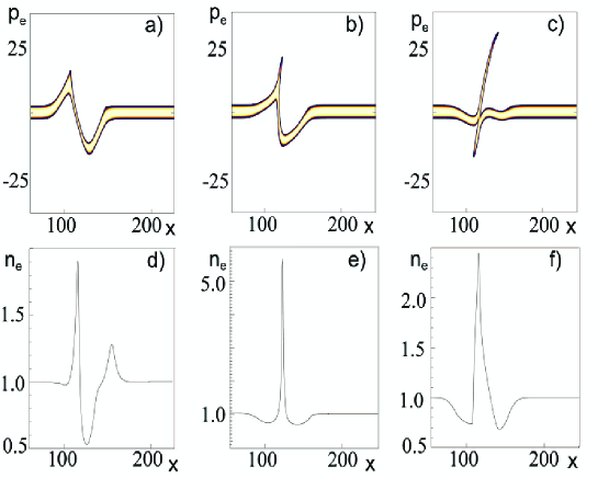
Figure 11: Results of 1D-Vlasov simulations of nonlinear wake wave breaking in thermal plasmas: electron phase plane in the plasma described by the waterbag distribution (a,b,c) and electron density profile (d,e,f) for $t=5,6,7$, respectively.

VI.3 Simple model

Consideration of Fig. 11 showing the singularity structures formed during and after the wave breaking leads to the formulation of a simple model within whose framework we can explain analytically the main features seen in the electron density distribution. As we may see from Fig. 11 b the ”$\Lambda$-type breaking” in the phase plane, $p,X$, can be locally approximated by a superposition of two finite width stripes of parabolic and cubic form as is illustrated in Fig. 12 a. In other words, the waterbag distribution function is constant within the regions marked by the curves $p_{\pm}(X)$ given by equations

$$p_{\pm}^{2}/2=X\pm\Delta X/2$$ (105)

in the part corresponding to the parabolic behaviour and

$$p_{\pm}^{3}-r\,p_{\pm}=X-X_{c}\pm\Delta X/2$$ (106)

for the cubic part. The parameters $r$ and $X_{c}$ provide the overlapping of these two stripes at large $p$, with $\Delta X$ being the distribution width at $p=0$.

In order to parametrize these dependences we consider the electron motion in the frame of reference, where the singularity region is at rest. The parabolic stripe here can be described using an approximation of the integral of motion, $m_{e}c\gamma=m_{e}c\gamma_{0}+eEX$, in the vicinity of the reflection point, where $p\to 0$, i.e. $p^{2}/2=m_{e}c(\gamma_{0}-1)+eEX$. We find that $\Delta X$ in Eq. (105) is proportional to the width $\Delta p_{0}$ of the initial momentum distribution and inversely proportional to the electric field reflecting back the electrons in the wave breaking region: $\Delta X=(m_{e}c/eE)(\gamma_{+,0}-\gamma_{-,0})\approx\Delta p_{0}/eE$. In the laboratory frame of reference the distribution width is approximately $2\gamma_{\rm ph}$ times narrower.

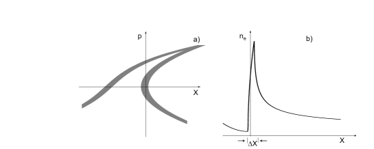
Figure 12: Simple model of the wave breaking: a) electron phase plane, b) electron density.

The electron density can be calculated as the area within the $p_{\pm}(X)$ curves. Its part corresponding to the parabolic curves is equal to

$$n_{e}(X)=n_{0}\frac{2\sqrt{2eEm_{e}c}}{\Delta p_{0}}\left[\theta\left(X+\frac{\Delta X}{2}\right)\sqrt{X+\frac{\Delta X}{2}}-\theta\left(X-\frac{\Delta X}{2}\right)\sqrt{X-\frac{\Delta X}{2}}\right],$$ (107)

where $\theta(x)$ is the Heaviside unit step function. The density reaches its maximum at $X=\Delta X/2$ with $n_{e,\max}=n_{0}\sqrt{m_{e}c/\Delta p_{0}}$. In the limit $X\gg\Delta X$ the electron density is inversely proportional to the square root of $X$, $n_{e}(X)\sim 1/\sqrt{X}$ as in the case corresponding to Eq. (102). In the laboratory frame of reference we have $n_{e,\max}=n_{0}\sqrt{m_{e}c\gamma_{\rm ph}^{3}/\Delta p_{0}}$. The contribution to the electron density from the cubic part of the distribution function is proportional to the surface of the area bounded by the curves $p_{\pm}(X)$ which are the roots of equation (106) given by the expressions

$$p_{\pm}(X)=\frac{2\,3^{1/3}r+2^{1/3}\left(\sqrt{81X_{\pm}^{2}-12r^{3}}-9X_{\pm}\right)^{2/3}}{6^{2/3}\left(\sqrt{81X_{\pm}^{2}-12r^{3}}-9X_{\pm}\right)^{1/3}}$$ (108)

with $X_{\pm}=X-X_{c}\pm\Delta X/2$, where $X$ is normalized on $mc/eE$ and $p$ measured in units of $m_{e}c$. At $X\gg\Delta p$ the electron density is proportional to $X^{-2/3}$, as in the case corresponding to Eq. (59).

We see an apparent similarity between the density distribution obtained with the computer simulations, which is shown in Fig. 11 f, and the density distribution given by the simple model (Fig. 12 b).

When $r=0$ the cubic part of the distribution function develops a new breaking point and for $r<0$ it is no longer a single valued functions of $X$. At $r=0$ the contribution of the cubic part results in the electron density described by

$$n_{e}(X)\sim\frac{n_{0}}{\Delta p_{0}}\left[\theta\left(X_{+}\right)\left(X_{+}\right)^{1/3}+\theta\left(-X_{-}\right)\left(-X_{-}\right)^{1/3}-\theta\left(X_{-}\right)\left(X_{-}\right)^{1/3}-\theta\left(-X_{+}\right)\left(-X_{+}\right)^{1/3}\right].$$ (109)

In the limit $\Delta p_{0}\to 0$ the electron density profile for $X\to 0$ is given by $n_{e}(X)\sim X^{-2/3}$ in accordance with the theory of the wave breaking in a cold plasma (see Eq. (59)).

VI.4 Energy scaling of laser accelerated electrons

Here we consider the LWFA acceleration in the above wave breaking regime when the wake field amplitude is not limited by the value $E_{\rm AP}$ (55) and is related via Eq. (95) for $\gamma_{\rm m}=1+a^{2}/2$ to the laser pulse amplitude as $E_{\max}=a$. The electron injected into the wakefield acceleration phase can acquire the energy ESL1

$${\cal E}=\frac{e\varphi_{w}}{1-\beta_{\rm ph}},$$ (110)

where the wakefield electrostatic potential is equal to $\varphi_{w}\approx 2\pi n_{0}e^{2}r_{w}^{2}$ with $r_{w}$ being the wakewave transverse size, which is of the order of the laser pulse waist equal to $r_{w}\approx(c/\omega_{\rm pe})\sqrt{2a}$. The amplitude of the laser pulse is given by Eq. (85). Using the relationship between the laser power and the amplitude (85) and between the wake wave phase velocity and the plasma density, which can be written as $\gamma_{\rm ph}=\sqrt{n_{\rm cr}a/n_{0}}$ (see Ref. EK ), we obtain for the accelerated electron energy

$${\cal E}\approx m_{e}c^{2}\left(\frac{\cal P}{{\cal P}_{c}}\right)^{2/3}\left(\frac{n_{\rm cr}}{n_{0}}\right)^{1/3}.$$ (111)

As we see, for given laser power the fast electron energy is proportional to $n_{0}^{-1/3}$, i.e. the lower plasma density, the higher the electron energy. The electron density cannot be lower than the density determining the relativistic self-focusing threshold (here we do not consider the laser wakefield excited inside a plasma waveguide, i.e. inside a plasma filled capillary), at which $n_{0,\min}=n_{\rm cr}{{\cal P}_{c}}/{\cal P}$ and $a\approx 1$, i.e. the wake plasma wave is in the weakly nonlinear regime as required for the laser based electron-positron collider LEPT , i.e. for $a\geq 1$. As the result, we obtain the electron energy scaling under the optimal conditions

$${\cal E}\approx m_{e}c^{2}\left(\frac{\cal P}{{\cal P}_{c}}\right),$$ (112)

which for ${\cal P}=50$TW yields ${\cal E}=3$GeV, and for ${\cal P}=100$PW gives ${\cal E}=6$TeV.

The acceleration length according to Eq. (110), $l_{\rm acc}=2r_{w}\gamma^{2}_{\rm ph}$, in the optimal regime is given by

$$l_{\rm acc}\approx\frac{\lambda}{\pi}\left(\frac{\cal P}{{\cal P}_{c}}\right)^{3/2}.$$ (113)

In the case of ${\cal P}=50$TW one-micron wavelength laser, we have $l_{\rm acc}\approx 5$cm.

We recall that in the limit of large laser amplitudes the energy scaling of the accelerated electrons in Eq. (112) has a different dependence on the laser plasma parameters as discussed in Ref. ESL1 and references quoted therein.

VII Discussions and Conclusions

In the present paper, by extending an approach formulated in Ref. RCD to the relativistic limit, we investigated the wave breaking of relativistically strong Langmuir wave in thermal plasmas. As is well known, the wavebreak concept is meaningful only for systems which allow the hydrodynamics description because in kinetic systems with broad distribution functions there are always processes similar to wave breaking, such as the Landau damping in linear and nonlinear regimes.

In the study of high power laser matter interaction wavebreak-like processes attract great attention in regimes where the wave amplitude is much larger than the distribution thermal spread in the momentum space, the most relevant questions being the maximal electric field, on the structure of the formed singularity and on the number of electrons involved in the wavebreaking.

Using the relativistic waterbag model we showed the typical structures of singularities occurring during the wave breaking, we found the dependence of maximum electric field on the wave parameters, and discussed the behaviour of nonlinear wave in collisionless plasmas. The approach based on the warm plasma fluid model ESL2 leads to the same scalings for the profile of the breaking waves.

We found that in the above breaking limit the electron distribution in the nonlinear wave takes a skewed form. Note the somewhat similar feature in breaking water waves, when a symmetric Stokes profile Stokes evolves to a skewed wave (see Ref. Whitham ).

- (1) V. L. Ginzburg, The Propagation of Electromagnetic Waves in Plasmas (Pergamon Press, Oxford, 1970); R. K. Dodd, J. C. Eilbeck, J. D. Gibbon, H. C. Norris, Solitons and Nonlinear Wave Equations (Academic Press Inc., New York, 1984); W. L. Kruer, Physics of Laser Plasma Interactions (Addison-Wesley, Menlo Park, CA, 1988); M. S. Longair, High Energy Astrophysics (Cambridge Univ. Press, Cambridge 1992).
- (2) T. Tajima and J. M. Dawson, Phys. Rev. Lett. 34, 269 (1979).
- (3) E. Esarey, C. B. Schroeder, W. P. Leemans, Rev. Mod. Phys. 81, 1229 (2009).
- (4) P. Chen, J. M. Dawson, R. W. Huff et al., Phys. Rev. Lett. 54, 693 (1985); T. Katsouleas, Phys. Rev. A 33,2056 (1986); I. Blumenfeld, C. E. Clayton, F.-J. Decker et al., Nature 445, 741 (2007).
- (5) D. F. Gordon, B. Hafizi, D. Kaganovich, A. Ting, Phys. Rev. Lett. 101, 045004 (2008); U. Teubner and P. Gibbon, Rev. Mod. Phys. 81, 445 (2009); A. S. Pirozhkov, M. Kando, T. Zh. Esirkepov et al., Phys. Rev. Lett. 108, 135004 (2012).
- (6) G. Mourou, T. Tajima, S. V. Bulanov, Rev. Mod. Phys. 78, 309 (2006).
- (7) S. V. Bulanov, T. Zh. Esirkepov, M. Kando, J. K. Koga, A. S. Pirozhkov, T. Nakamura, S. S. Bulanov, C. B. Schroeder, E. Esarey, F. Califano, and F. Pegoraro, Phys. Plasmas (2012) - submitted for publication; [arXiv e-print: 2012ArXiv1202.1907B].
- (8) A. I. Akhiezer and R. V. Polovin, Sov. Phys. JETP 30, 915 (1956).
- (9) S. V. Bulanov, V. I. Kirsanov, A. S. Sakharov, JETP Letters 53, 565 (1991).
- (10) R. C. Davidson, Methods in nonlinear plasma theory (Academic Press Inc., New York, 1972).
- (11) J. M. Dawson, Phys. Rev. 113, 383 (1959).
- (12) T. Katsouleas and W. Mori, Phys. Rev. Lett. 61,90 (1988).
- (13) S. V. Bulanov, I. N. Inovenkov, V. I. Kirsanov et al., Phys. Fluids B 4, 1935 (1992); C. A. Coverdale, C. B. Darrow, C. D. Decker et al., Phys. Rev. Lett. 74, 4659 (1995); A. Modena, A. Najmudin, E. Dangor et al., Nature (London) 377, 606 (1995); S. V. Bulanov, F. Pegoraro, A. M. Pukhov, A. S. Sakharov, Phys. Rev. Lett. 78, 4205 (1997); D. Gordon, K. C. Tzeng, C. E. Clayton et al., Phys. Rev. Lett. 80, 2133 (1998); S. V. Bulanov, N. Naumova, F. Pegoraro, J. Sakai, Phys. Rev. E 58, R5257 (1998); H. Suk, N. Barov, J. B. Rosenzweig, E. Esarey, Phys. Rev. Lett. 86, 1011 (2001); A. Pukhov and J. Meyer-Ter-Vehn, Appl. Phys. B 74, 355 (2002); M. C. Thompson, J. B. Rosenzweig, H. Suk, Phys. Rev. ST Accel. Beams 7, 011301 (2004); P. Tomassini, M. Galimberti, A. Giulietti et al., Laser Part. Beams 22, 423 (2004); T. Ohkubo, A. G. Zhidkov, T. Hosokai et al. Phys. Plasmas 13, 033110 (2006); M. Kando, Y. Fukuda, H. Kotaki, et al., JETP, 105, 916 (2007); C. G. R. Geddes, K. Nakamura, G. R. Plateau et al., Phys. Rev. Lett. 100, 215004 (2008); A. V. Brantov, T. Zh. Esirkepov, M. Kando et al., Phys. Plasmas 15, 073111 (2008); J. Faure, C. Rechatin, O. Lundh et al., Phys. Plasmas 17, 083107 (2010); K. Schmid, A. Buck, C. M. S. Sears, et al. Phys. Rev. ST Accel. Beams 13, 091301 (2010); Y.-C. Ho, T.-S. Hung, C.-P. Yen et al., Phys. Plasmas 18, 063102 (2011); A. J. Gonsalves, K. Nakamura, C. Lin et al., Nature Phys. 7, 862 (2011); Y. Y. Ma, S. Kawata, T. P. Yu, et al., Phys. Rev. E 85, 046403 (2012).
- (14) C. B. Schroeder, E. Esarey, B. A. Shadwick, Phys. Rev. E 72, 055401 (2005); C. B. Schroeder, E. Esarey, B. A. Shadwick, W. P. Leemans, Phys. Plasmas 13, 033103 (2006); C. B. Schroeder, E. Esarey, B. A. Shadwick, Phys. Plasmas 14, 084701 (2007); C. B. Schroeder and E. Esarey, Phys. Rev. E 81, 056403 (2010).
- (15) R. M. G. M. Trines and P. A. Norreys, Phys. Plasmas 13, 123102 (2006); R. M. G. M. Trines and P. A. Norreys, Phys. Plasmas 14, 084702 (2007); R. M. G. M. Trines, Phys. Rew. E 79, 056406 (2009); R. M. G. M. Trines, R. Bingham, Z. Najmudin et al. New Jornal of Physics 12, 045027 (2010); Z. M. Sheng and J. Meyer-ter-Vehn, Phys. Plasmas 4, 493 (1997).
- (16) T. P. Coffey, Phys. Fluids 14, 1402 (1971); T. Coffey, Phys. Plasmas 17, 052303 (2010);
- (17) D. A. Burton and A. Noble, J. Phys. A: Math. Theor. 43, 075502 (2010).
- (18) A. A. Solodov, V. M. Malkin, N. J. Fisch, Phys. Plasmas 13, 093102 (2006).
- (19) A. V. Panchenko, T. Zh. Esirkepov, A. S. Pirozhkov et al., Phys. Rev. E 78, 056402 (2008).
- (20) B. Riemann, Abhandlungen der Königlichen Gesellschaft der Wissenschaften zu Göttingen, 8, 43 (1860).
- (21) L. D. Landau and E. M. Lifshitz, Fluid Mechanics (Butterworth and Heinemann, Oxford, 1987).
- (22) G. G. Stokes, Trans. Cambridge Philos. Soc. 8, 441 (1847); J. Wilkening, Phys. Rev. Lett. 107, 184501 (2011).
- (23) G. B. Whitham, Linear and Nonlinear Waves (Wiley-Interscience, New York, 1974).
- (24) R. Camassa and D. D. Holm, Phys. Rev. Lett. 71, 1661 (1993).
- (25) L. V. Keldysh, Sov. Phys. JETP 20, 1307 (1965); V. S. Popov, Phys. Usp. 47, 855 (2004).
- (26) J. K. Koga et al., in preparation.
- (27) F. Pegoraro and F. Porcelli, Phys. Fluids, 27, 1665 (1984).
- (28) B. Buti Phys. Fluids, 5, 1 (1962).
- (29) T. Nakamura, M. Tampo, R. Kodama et al., Phys. Plasmas 17, 113107 (2010).
- (30) A. Zhidkov, J. Koga, K. Kinoshita, M. Uesaka, Phys. Rev. E 69, 035401(R) (2004).
- (31) G. A. Askar’yan, Sov. Phys. JETP 15, 1088 (1962); A. G. Litvak, Sov. Phys. JETP 30, 344 (1969); C. E. Max, J. Arons, A. B. Langdon, Phys. Rev. Lett. 33, 209 (1974); P. Sprangle, C. M. Tang, E. Esarey, IEEE Trans. Plasma Sci. 15, 145 (1987); G. Z. Sun, E. Ott, Y. C. Lee, P. Guzdar, Phys. Fluids 30, 526 (1987); A. B. Borisov, A. V. Borovskiy, V. V. Korobkin et al., Phys. Rev. Lett. 65, 1753 (1990); P. Monot, T. Auguste, P. Gibbon et al., Phys. Rev. Lett. 74, 2953 (1995).
- (32) A. Mangeney, F. Califano, C. Cavazzoni, P. Travnicek, J. Comp. Physics 179, 495 (2002).
- (33) S. S. Bulanov, V. Yu. Bychenkov, V. Chvykov et al., Phys. Plasmas 17, 043105 (2010).
- (34) M. Abramowitz and I. A. Stegun, Handbook of Mathematical Functions with Formulas, Graphs, and Mathematical Tables (Dover, New York, 1964).
- (35) W. Leemans and E. Esarey, Physics Today 62, 44 (2009).