A Two-Dimensional Infrared Map of the Extrasolar Planet HD 189733b

Abstract

We derive the first secondary eclipse map of an exoplanet, HD 189733b, based on Spitzer IRAC 8 micron data. We develop two complementary techniques for deriving the two dimensional planet intensity: regularized slice mapping and spherical harmonic mapping. Both techniques give similar derived intensity maps for the infrared day-side flux of the planet, while the spherical harmonic method can be extended to include phase variation data which better constrain the map. The longitudinal offset of the day-side hot spot is consistent with that found in prior studies, strengthening the claim of super-rotating winds, and eliminating the possibility of phase variations being caused by stellar variability. The latitude of the hot-spot is within 10.1^∘ (68% confidence) of the planet’s equator, confirming the predictions of general circulation models for hot Jupiters and indicative of a small planet obliquity.

1. Introduction

One of the great challenges in studying extrasolar planets is that we cannot directly resolve the surfaces of these bodies. This is a common problem in astronomy, and one solution is to use occultations or eclipses to spatially resolve astronomical sources. Eclipse mapping has been applied variously to map stars (e.g. Schmitt & Kurster, 1993; Lanza et al., 1998), accretion disks (e.g. Horne, 1985), planetary satellites (e.g. Aksnes & Franklin, 1975), dwarf planets (e.g. Young et al., 1999, 2001), and unresolved radio sources (e.g. Taylor, 1966, 1967). Here we present the first eclipse map of an extrasolar planet.

The secondary eclipse is the decrease in flux that occurs when a planet passes behind its host star. The eclipse ingress and egress contain information about the spatial distribution of the planet’s day side flux. For example, a planet with a brighter western hemisphere has an apparent delay in the times of ingress and egress, and a modified shape of the ingress and egress. This delay in eclipse timing due to a zonally asymmetrical planet was predicted by Williams et al. (2006) and first observed by Knutson et al. (2007) and Agol et al. (2010). In addition to this artificial time offset, the ingress/egress morphology may be used to map exoplanets as pointed out in Rauscher et al. (2007).

Longitudinal variations in the brightness of the planet cause a variation in the brightness of the planet with orbital phase. This orbital modulation has been observed in transiting (Knutson et al., 2007, 2009b, 2009a) and non-transiting systems (Cowan et al., 2007; Crossfield et al., 2010). Cowan & Agol (2008) described how to invert such phase variations into a low-resolution longitudinal map of a planet; the first such map was presented in Knutson et al. (2007).

1.1. The Hot Jupiter HD 189733b

The short-period transiting jovian planet HD 189733b (Bouchy et al., 2005) is one of the first planets to have been detected in infrared emission during secondary eclipse (Deming et al., 2006), and has been studied in depth since that detection (Knutson et al., 2007; Grillmair et al., 2008; Charbonneau et al., 2008; Knutson et al., 2009b; Agol et al., 2010; Désert et al., 2011).

We apply our mapping techniques to the seven secondary eclipse measurements of Agol et al. (2010) and, in the case of spherical harmonic mapping, the phase measurement presented in Knutson et al. (2007). These data have been corrected for detector effects and stellar variability, and the seven eclipse light curves were binned in phase to 644 points. To this we appended the phase variation data from Knutson et al. (2007), binned by 275.

2. Eclipse mapping

2.1. Model Assumptions

Three conditions need to be satisfied in order to construct an eclipse map: the planet emission pattern must be static, the time of superior conjunction must be known, and the planet limb-darkening must be negligible.

A static diurnal temperature pattern is required for any form of thermal mapping. Most general circulation models (GCMs) for hot Jupiters indicate $<1$% variability (Showman & Guillot, 2002; Cooper & Showman, 2005; Showman et al., 2009; Dobbs-Dixon et al., 2010), while observations of multiple secondary eclipses of HD 189733b indicate that the eclipse depth does not vary significantly, $<2.7$% over a period of more than 500 days (Agol et al., 2010). Hence the static map assumption is likely justified for this planet.

Eclipse mapping can be applied provided that the time of superior conjunction is known to a few seconds, which is beyond the precision of radial velocity measuremenents. We assume a circular orbit, hence pegging the time of eclipse to the time of transit which is precisely known. This assumption can then be checked by comparing the phase-function and secondary eclipse maps, and seems to apply for HD 189733b (Agol et al., 2010).

Ignoring the effect of limb darkening is required so that the surface brightness of a location on the planet does not change as the planet rotates. This assumption is not required for our slice-mapping technique, since in that case we implicitly neglect changes in the planet’s phase. Regardless, limb darkening is thought to be very weak for hot Jupiters, about 20% linear limb-darkening, especially in the wavelength of the observations (8 micron), so this assumption is likely reasonable for HD 189733b, as we show below.

In addition to these assumptions about the planet, we assume some things of the data. Any stellar variability must be corrected for, which may not be possible if it has a period close to that of the planet. We have corrected for stellar variability using the correlation between optical and infrared flux variations as discussed in Agol et al. (2010). Detector ramp and other detector-related effects are corrected for as described in Agol et al. (2010). Additionally, all light curves henceforth are taken to have the stellar flux subtracted off, so that measurements when the planet is completely occulted have zero value.

We describe two approaches to planet mapping: (1) slice mapping (§2.2); (2) spherical harmonic mapping (§2.3).

Figure 1.— Top: diagram demonstrating the slice mapping technique. If one adopts the convention that North points in the direction of the planet’s rotational angular momentum, then western regions of the planet are occulted first during ingress, and revealed first during egress (for a tidally-locked planet the rotational and orbital angular momenta are identical). If North points up and East to the right, then ingress is on the right and egress on the left; time therefore runs from right to left. Bottom: Ingress and egress maps (right and left), as well as a combined map (center) of HD 189733b at 8 $\mu$m. The image is centered on the sub-observer point and the black regions are 50% as bright as the white.

2.2. The Slice Method

During a time interval within ingress/egress, we can compute the area of the planet that disappears/appears behind the star if we assume a circular orbit. The fraction of flux that disappears during that time interval is then proportional to the mean surface brightness of the area that disappeared. This is the basis of our first mapping technique.

As a planet passes behind its star, the light curve flux, $F(t)$, at any given time may be associated with the roughly crescent-shaped portion of its day side currently visible to the earth. It is thus proportional to the planet’s light distribution function, $I(\theta,\phi)$, integrated over the visible area, $A(t)$. If we take two successive observations at times $t_{j-1}$ and $t_{j}$, the change in observed flux, $\Delta F_{j}=F(t_{j})-F(t_{j-1})$, is due solely to the change in area $\Delta A_{j}=A(t_{j})-A(t_{j-1})$ times the intensity averaged over that area. The average intensity, $\bar{I}_{j}$, over the slice with area $\Delta A_{j}$ is then given by $\bar{I}_{j}=\Delta F_{j}/\Delta A_{j}$.

We partition the planet’s ingress and egress into observations at a finite number of intervals, $\Delta t_{j}$, and from these calculate each $\bar{I}_{j}$, yielding two ‘slice maps’: 1D maps of the planet day side. This process and its results for HD 189733b are shown in Figure 1.

Once these maps were found, we combined them into a single 2-dimensional map of the planet, forming a grid of the ingress and egress slices. This step of the inversion requires a prior since if the ingress and egress maps are each made from $N$ slices, the combined map contains roughly $N^{2}$ cells. We assume that the planet’s intensity distribution varies smoothly, which is imposed via linear regularization, in which a solution is chosen that is consistent with the data and has the smallest differences between adjacent slices. We use a goodness of fit parameter of $\chi^{2}+\lambda\sum_{i}({\bar{I}_{i}}-{\bar{I}_{i-1}})^{2}$. We chose a regularization coefficient, $\lambda=100$, to give a reduced chi-square of order unity, resulting in the map of HD 189733b shown in Figure 1.

2.3. Spherical harmonic mapping

Our second method for extracting a map from the eclipse light curve uses spherical harmonics. We applied this to two data sets: 1) only the secondary eclipse data; 2) both the secondary eclipse and phase-function data.

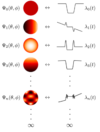
Figure 2.— A few spherical harmonics and their corresponding ‘harmonic light curves,’ $(\lambda_{0},\lambda_{1},\lambda_{2},...)$.

Taking $I(\theta,\phi)$ to be the intensity map of a transiting extrasolar planet, we may approximate it to an arbitrary degree of accuracy by truncating its harmonic sum at some finite number of terms, $0\leq l\leq l_{max}$, with $-l\leq m\leq l$. We compute the light curve that would be observed if the planet’s map consisted solely of each harmonic, and then solve for the coefficients of each harmonic light curve from the data via linear regression. We implemented the light curve calculation using the HEALPix IDL package, which contains routines for the evaluation and projection of spherical harmonics (Górski et al., 2005). The map is then formed by transforming back to the harmonics and summing the result. This transformation is portrayed graphically in Figure 2, and the results of its application to observations of HD 189733b can been seen in Figure 4. This is essentially a two dimensional generalization of the Fourier decomposition technique for phase mapping developed in Cowan & Agol (2008); note that the 2D image shown in Knutson et al. (2007) only contained longitudinal information, while the latitudinal depdence was arbitrarily chosen.

We generate the light curve for the real spherical harmonics, $\Psi_{i}$ (where $i$ labels the harmonics used in our inversion) by painting a planet with a particular harmonic and then stepping through the planet’s orbit for each of the observed orbital phases. At each phase the harmonic is integrated over the visible portion of the planet to get the total flux that would be observed. We integrate over the visible area by finding a function with curl equal to the harmonic and integrate it around the area’s boundary, which is simply the concatenation of two known arcs, using Green’s Theorem. This technique yields both the planet phase variation and secondary eclipse shape for each harmonic, as shown in Figure 2.

With a set of $n$ spherical harmonic light curves, $\lambda_{1}(t),...,\lambda_{n}(t)$, we decompose the observed light curve, $F(t)$, by computing the the coefficients $c_{1},...,c_{n}$ as $c_{i}=\int F(t)\lambda_{i}(t)dt.$ These translate directly to the map’s coefficients for the harmonics $\Psi_{1},...,\Psi_{n}$. By adding the terms together we form a best-fit map of the entire planet, the closest approximation we can reach using the chosen harmonics, shown in Figure 4.

For the HD 189733b Channel 4 IRAC map, we chose to use only the first four harmonics $(l,m)={(0,0),(1,-1),(1,0),(1,1)}$ which gave a reduced chi-square of the fit close to unity. Thus, the maps only contain a dipole variation in flux, which corresponds to the “hot spot” feature seen in simulations and inferred from the phase function.

To quantify the statistical uncertainty on the measured hot spot location, we ran a Markov chain using the spherical harmonic fits. Beginning with a uniformly bright planet in a 4-dimensional vector space corresponding to the first four harmonic coefficients, we attempted jumps with magnitude based upon the uncertainty found in the initial decomposition for each coefficient, and a jump factor adjusted every 100 steps to achieve and acceptance rate of $\approx 44$%, with the acceptance criterion based on the Metropolis-Hastings algorithm. The longitudinal and latitudinal positions of the hottest point on the planet model was recorded for each of the 25,000 iterations, and the resulting distribution is plotted in Figure 3.

It is not known whether the orbital angular momentum of the system is tilted towards or away from the observer, so we are only able to constrain the distance of the hot spot from the equator, not specify whether it is in the northern or southern hemisphere. Accounting for this degeneracy, we find a hot spot latitude within $21.1$ degrees of the equator for the secondary eclipse inversion, albeit with a slight preference for off-equatorial locations, and within $10.1$ degrees of the equator for the eclipse-plus-phase inversion.

The corresponding longitude was $27.1^{+43.5}_{-9.0}$ deg East and $21.8\pm 1.5$ deg East for the eclipse or eclipse plus phase inversion, respectively. Consequently, the phase function gives significant leverage in constraining both the longitude and latitude of the hot spot.

Thermal phase variations are completely “blind” to meridional (N–S) brightness variations, so it is worth explaining how these data improve the constraints on the latitude of the hot spot. Due the planet’s non-zero impact parameter, the star’s limb scans diagonally across the planet, so eclipse mapping is unable to break the degeneracy between zonal (E–W) and meridional concentration of the dayside flux. The ingress and egress maps (Figure 1) scan in complementary directions, however, and therefore could distinguish between a zonal and meridional offset of the hotspot. Nevertheless, there remains a partial degeneracy between zonal/meridional concentration and hot spot offset. By measuring the zonal brightness concentration and longitude of the hot spot, phase variations break this degeneracy, leading to stronger constraints on the latitude of the hotspot.

In any case, we estimate that both hot spot longitude and latitude are subject to $\approx 15$% systematic errors due to neglect of $l>1$ modes in the inversion based on our simulated data, as described next.

Figure 3.— Probability distribution for the longitude and latitude of the hot spot in the $l_{\rm max}=1$ spherical harmonic maps based on the secondary eclipse (solid lines) and secondary eclipse plus phase function (dashed lines). Angles are measured in the rotation frame of the planet, with the origin at the sub-stellar point. It is not known whether the orbital angular momentum of the system is tilted towards or away from the observer, so we are only able to constrain the distance of the hot spot from the equator, not specify whether it is in the northern or southern hemisphere.

3. Application to Simulated Data

We created simulated light curves using a two dimensional map at constant pressure from a GCM for a hot Jupiter planet (Showman et al., 2008), to which we applied the spherical harmonic mapping technique. We took a snap shot of the temperature at 100 mbar from a simulation, converted it to surface brightness in the Rayleigh-Jeans limit, and then created a simulated light curve from the images. The light curve was computed for identical orbital and size parameters as HD 189733a,b and for the same range of phase that was observed (about 1/3 of the planet’s orbit prior to secondary eclipse), and we assumed that the planet has a fixed temperature pattern with no limb-darkening, as well as a circular orbit and spherical bodies. We carried out six different versions of the simulated light curves: 1) we first decomposed the temperature map into spherical harmonics up to order $l_{max}$, and then used the map based on only these harmonics to compute a light curve with no noise; 2) we computed the same light curve, but with noise added at the level of the observed data from Agol et al. (2010); 3) same as 2, but we shifted the hot spot North in latitude by 12, 23, 40 and 60 degrees; 4) we computed a light curve using the full temperature map; 5) we added noise to the light curve using the full map; 6) we carried out an identical test as version 1, but with 20% linear limb-darkening. We found that for $l_{max}=1$, we could recover the correct coefficients of the spherical harmonics in version 1, which shows that the code performed as expected. When noise was added, we found a scatter in the derived parameters at the 10% level. With $l_{max}=2$, we found that the derived spherical harmonics became very poorly constrained, likely due to degeneracies in the harmonic light curves, so for the remainder of the analysis we used $l_{max}=1$ when extracting the map. For version 3, we ran 100 simulations at each latitudinal offset, and found that the mean of the recovered latitudes matched the input value, with a scatter varying from 12 deg RMS at the equator to 6 deg nearer to the pole. For version 4, we found that the amplitude of the spherical harmonics relative to the $(0,0)$ component had systematic errors as large as $\approx 50$%. However, the amplitude of the spherical harmonics relative to the day-side flux inferred from the map agreed to better than 15%, while the location of the hot spot differed by $\approx 10-15$% in longitude and latitude. For version 5 we found that the statistical error did not change much for $l_{max}=1$, still at the 10% level. For version 5, we find that 20% limb darkening affects the derived coefficients by less than 5%.

Based on these tests, we are confident in our inference of the longitude and latitude of the planet hot spot the dipole amplitude relative to the day-side flux at the $\approx 15$% level. Additionally, we confirm the validity of our assumption to ignoring the effects of limb darkening for hot Jupiters in 8 micron.

4. Discussion and Conclusions

4.1. Slice vs. Spherical Harmonic Eclipse Maps

The fact that the slice map (Figure 1) and spherical harmonic map (Figure 4) give qualitatively similar results is reassuring as the two techniques have very different assumptions and potential systematic errors. Both maps favor a hot spot that is offset slightly latitudinally; however, when the phase function is included in the analysis, this constrains the spot to be located more closely to the equator. This is due to the fact that the phase function provides a strong constraint on the longitudinal variation of the planet brightness, and thus does not allow as much freedom in varying both the longitude and latitude to fit the secondary eclipse.

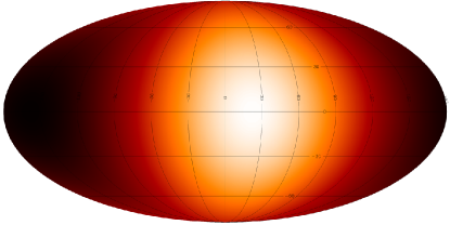
Figure 4.— A Molleweide projection of the 2D infrared map of HD 189733b with $l_{max}=1$; latitude and longitude lines are spaced every 30^∘. Coordinates are centered on the sub-stellar point and intensity values are relative (white is brightest, black is 30.2% as bright).

The slice map has the disadvantage that it does not account for the rotation of the planet or the tilt of the planet, nor can it be used in conjunction with the phase variation of the planet, resulting in the north-south asymmetry visible in the slice map above absent from the harmonic mapping results. In addition, it is difficult to derive uncertainties on the intensity, which are highly correlated due to the regularization.

The spherical harmonic method has the advantage of being able to easily account for these effects, but the disadvantage that it assumes to a large degree that the planet intensity varies smoothly as we are constrained to use small $l_{max}$, in this case $l_{max}=1$.

4.2. Phase versus Eclipse Mapping

Phase mapping (Cowan & Agol, 2008) offers more leverage on the longitudinal brightness distribution of the planet than does eclipse mapping. This is because the same change in flux is spread out over an orbital period, $P$, rather than the duration of ingress/egress, $\tau_{ing}$, allowing for greater signal-to-noise constraints given the same photometric uncertainties. The ratio of these two timescales is $\tau_{\rm ing}/P\propto R_{p}/(\pi a)$ ($\approx$0.4% for HD 189733), where $R_{p}$ and $a$ are the planetary radius and orbital semi-major axis, respectively. Whenever it is feasible to obtain photometry throughout an entire orbit (or a sizable fraction thereof), phase curve inversion will provide the best estimate of the hottest and coldest local stellar times. This will be especially true as one tries to apply these techniques to smaller planets with longer periods.

Eclipse mapping offers three significant advantages over phase mapping, however:

1) Eclipse mapping is sensitive to to the latitudinal intensity distribution on a planet if it has non-zero impact parameter as it passes behind the disk of its star.

2) The planet’s brightness map is assumed to be static over the eclipse duration, $\tau_{\rm ecl}$, which is much shorter than that assumed for phase mapping, $P$, and thus influenced less by other forms of variability. The ratio of these two timescales is $\tau_{\rm ecl}/P\propto R_{*}/a$ ($\approx$ 3% for HD 189733). While there is no clear evidence yet for weather on transiting planets, it will certainly be the case that the intensity distributions of eccentric planets as seen by an observer will vary throughout an orbit. Eclipse mapping therefore offers the only prospect for constraining the intensity distributions of this intriguing class of objects.

3) There is no theoretical limit to the spatial resolution one can achieve with eclipse mapping, although there may be some degeneracy as we have found. This is in stark contrast to phase mapping, where one runs into fundamental degeneracies with odd harmonics after only 5 terms (Cowan & Agol, 2008).

4.3. Summary

We developed two techniques for converting an observed secondary eclipse light curve into a two-dimensional map of a planet.

The spherical harmonic formalism is a robust way to make an exoplanet map from secondary eclipse light curves, and can accommodate observations of thermal phase variations. Slice maps may also be constructed at ingress and egress, then combined via regularization. While this technique seems to produce comparable day-side maps for the data at hand, it is not as robust or versatile as the spherical harmonic technique.

We applied both mapping techniques to the transiting planet HD 189733b. We find that the primary day-side hotspot is offset to the East by 21.8(1.5)^∘, in agreement with the phase variation measurements of Knutson et al. (2007) and the eclipse timing constraint from Agol et al. (2010). The data indicate a hot spot within $10.1^{\circ}$ of the equator. The fact that the hottest point lies close to the equator is consistent with a small obliquity of the planet as oblique rotators are predicted to show strong latitudinal contrast (Langton & Laughlin, 2007); this conclusion is also consistent with theoretical computations which predict a small obliquity for hot Jupiters (Fabrycky et al., 2007; Levrard et al., 2007). Taken together, these studies strongly favor super-rotating winds in the vicinity of the 8 micron photosphere, as predicted in GCMs (Cooper & Showman, 2005; Showman et al., 2008; Showman et al., 2009; Rauscher & Menou, 2010; Burrows et al., 2010; Showman & Polvani, 2011). The mapping codes used in this paper, written in IDL, are available from the authors upon request; however, the assumptions that go into this planet mapping technique need to be verified for other planets studied.

References

- Agol et al. (2010) Agol, E., Cowan, N. B., Knutson, H. A., Deming, D., Steffen, J. H., Henry, G. W., & Charbonneau, D. 2010, ApJ, 721, 1861
- Aksnes & Franklin (1975) Aksnes, K. & Franklin, F. A. 1975, AJ, 80, 56
- Bouchy et al. (2005) Bouchy, F., Udry, S., Mayor, M., Moutou, C., Pont, F., Iribarne, N., da Silva, R., Ilovaisky, S., Queloz, D., Santos, N. C., Ségransan, D., & Zucker, S. 2005, A&A, 444, L15
- Burrows et al. (2010) Burrows, A., Rauscher, E., Spiegel, D. S., & Menou, K. 2010, ApJ, 719, 341
- Charbonneau et al. (2008) Charbonneau, D., Knutson, H. A., Barman, T., Allen, L. E., Mayor, M., Megeath, S. T., Queloz, D., & Udry, S. 2008, ApJ, 686, 1341
- Cooper & Showman (2005) Cooper, C. S. & Showman, A. P. 2005, ApJ, 629, L45
- Cowan & Agol (2008) Cowan, N. B. & Agol, E. 2008, ApJ, 678, L129
- Cowan et al. (2007) Cowan, N. B., Agol, E., & Charbonneau, D. 2007, MNRAS, 379, 641
- Crossfield et al. (2010) Crossfield, I. J. M., Hansen, B. M. S., Harrington, J., Cho, J. Y.-K., Deming, D., Menou, K., & Seager, S. 2010, ApJ, 723, 1436
- Deming et al. (2006) Deming, D., Harrington, J., Seager, S., & Richardson, L. J. 2006, ApJ, 644, 560
- Désert et al. (2011) Désert, J.-M., Sing, D., Vidal-Madjar, A., Hébrard, G., Ehrenreich, D., Lecavelier Des Etangs, A., Parmentier, V., Ferlet, R., & Henry, G. W. 2011, A&A, 526, A12+
- Dobbs-Dixon et al. (2010) Dobbs-Dixon, I., Cumming, A., & Lin, D. N. C. 2010, ApJ, 710, 1395
- Fabrycky et al. (2007) Fabrycky, D. C., Johnson, E. T., & Goodman, J. 2007, ApJ, 665, 754
- Górski et al. (2005) Górski, K. M., Hivon, E., Banday, A. J., Wandelt, B. D., Hansen, F. K., Reinecke, M., & Bartelmann, M. 2005, ApJ, 622, 759
- Grillmair et al. (2008) Grillmair, C. J., Burrows, A., Charbonneau, D., Armus, L., Stauffer, J., Meadows, V., van Cleve, J., von Braun, K., & Levine, D. 2008, Nature, 456, 767
- Horne (1985) Horne, K. 1985, MNRAS, 213, 129
- Knutson et al. (2007) Knutson, H. A., Charbonneau, D., Allen, L. E., Fortney, J. J., Agol, E., Cowan, N. B., Showman, A. P., Cooper, C. S., & Megeath, S. T. 2007, Nature, 447, 183
- Knutson et al. (2009a) Knutson, H. A., Charbonneau, D., Cowan, N. B., Fortney, J. J., Showman, A. P., Agol, E., & Henry, G. W. 2009a, ApJ, 703, 769
- Knutson et al. (2009b) Knutson, H. A., Charbonneau, D., Cowan, N. B., Fortney, J. J., Showman, A. P., Agol, E., Henry, G. W., Everett, M. E., & Allen, L. E. 2009b, ApJ, 690, 822
- Knutson et al. (2011) Knutson, H. A., Madhusudhan, N., Cowan, N. B., Christiansen, J. L., Agol, E., Deming, D., Désert, J.-M., Charbonneau, D., Henry, G. W., Homeier, D., Langton, J., Laughlin, G., & Seager, S. 2011, ApJ, 735, 27
- Langton & Laughlin (2007) Langton, J. & Laughlin, G. 2007, ApJ, 657, L113
- Lanza et al. (1998) Lanza, A. F., Catalano, S., Cutispoto, G., Pagano, I., & Rodono, M. 1998, A&A, 332, 541
- Levrard et al. (2007) Levrard, B., Correia, A. C. M., Chabrier, G., Baraffe, I., Selsis, F., & Laskar, J. 2007, A&A, 462, L5
- Rauscher et al. (2007) Rauscher, E., Menou, K., Seager, S., Deming, D., Cho, J., & Hansen, B. M. S. 2007, ApJ, 664, 1199
- Rauscher & Menou (2010) Rauscher, E., & Menou, K. 2010, ApJ, 714, 1334
- Schmitt & Kurster (1993) Schmitt, J. H. M. M. & Kurster, M. 1993, Science, 262, 215
- Showman & Polvani (2011) Showman, A. P., & Polvani, L. M. 2011, ApJ, 738, 71
- Showman et al. (2009) Showman, A. P., Fortney, J. J., Lian, Y., et al. 2009, ApJ, 699, 564
- Showman et al. (2008) Showman, A. P., Cooper, C. S., Fortney, J. J., & Marley, M. S. 2008, ApJ, 682, 559
- Showman & Guillot (2002) Showman, A. P. & Guillot, T. 2002, A&A, 385, 166
- Taylor (1967) Taylor, J. H. 1967, ApJ, 150, 421
- Taylor (1966) Taylor, Jr., J. H. 1966, ApJ, 146, 646
- Williams et al. (2006) Williams, P. K. G., Charbonneau, D., Cooper, C. S., Showman, A. P., & Fortney, J. J. 2006, ApJ, 649, 1020
- Young et al. (2001) Young, E. F., Binzel, R. P., & Crane, K. 2001, AJ, 121, 552
- Young et al. (1999) Young, E. F., Galdamez, K., Buie, M. W., Binzel, R. P., & Tholen, D. J. 1999, AJ, 117, 1063