Applying quantum mechanics to macroscopic and mesoscopic systems

Abstract

There exists a paradigm in which Quantum Mechanics is an exclusively developed theory to explain phenomena on a microscopic scale. As the Planck’s constant is extremely small, $h\sim 10^{-34}$ J.s, and as in the relation of de Broglie the wavelength is inversely proportional to the momentum; for a mesoscopic or macroscopic object the Broglie wavelength is very small, and consequently the undulatory behavior of this object is undetectable. In this paper we show that with a particle oscillating around its classical trajectory, the action is an integer multiple of a quantum of action, $S=nh_{o}$. The quantum of action, $h_{o}$, which plays a role equivalent to Planck’s constant, is a free parameter that must be determined and depends on the physical system considered. For a mesoscopic and macroscopic system: $h_{o}\gg h$, this allows us to describe these systems with the formalism of quantum mechanics.

I Introduction

With Fermat’s principle, for the trajectory of an optical ray, the eikonal equation of the geometric optics is obtained and with the principle of stationary action (or principle of minimum action), for the trajectory of particles, the Hamilton-Jacobi equation is obtained; the two equations set up a link between geometrical optics and classical mechanics. L. de Broglie postulated in 1924 that a particle can have wave properties (duality wave-particle) De-Broglie , the experimental confirmation of this phenomenon led Schrödinger to postulate an equation for the De Broglie associated wave, called Schrödinger equation, in which a macroscopic scale could be reduced to the classical mechanics of a particle Schrodinger , this gave origin to undulatory mechanics. With the collaboration of M. Born and P. Jordan, W. Heisenberg Heisenberg establishes an equivalent theory known as matrix mechanics. Nowadays, both theories, undulatory and matrix mechanics, are known by the generic name of quantum mechanics. From the beginning quantum mechanics has been accompanied by much controversy, mainly with respect to the conceptual meaning of the mathematical formulations, leading to various interpretations (Copenhagen, statistics, and others), nevertheless, there is no doubt of its validity for its effectiveness in describe and predict various experimental results.

M. Born interpreted the square of the wavefunction as the probability density of finding a particle Born , and with this he was able to overcome the rupture existing between matrix and undulatory mechanics; in addition it allowed to establish an analogy between the temporary evolution of the probability functions and those of a hydrodynamic fluid. The hydrodynamic formulation of quantum mechanics was initiated with E. Madelung Madelung , which was later used by D. Bohm Bohm ; in this formulation, the Schrödinger equation is reduced to the Hamilton-Jacobi equation. The Hamilton-Jacobi equation shows that particles of the ensemble are subject, not only, to a "potential classic" but also to a "quantum potential" that give rise to forces that determine the evolution of each particle. The lack of knowledge about how to obtain the quantum potential has blocked the development of the hydrodynamic formulation of the quantum mechanics, for this reason it has been restricted to philosophical and epistemological discussions, and to the interpretation of the results obtained by numerical integration, however, were found some applications in the area of physical chemistry Aplicaciones .

There exists a paradigm in which Quantum Mechanics are an exclusively developed theory to explain phenomena on a microscopic scale. As the Planck’s constant is extremely small, $h\sim 10^{-34}$ J.s, and as in the relation of de Broglie the wavelength is inversely proportional to the momentum; for a mesoscopic or macroscopic object the Broglie wavelength is very small, and consequently the undulatory behavior of this object is undetectable. For this reason, in a mesoscopic or macroscopic system, the quantum mechanics reduces to classical mechanics. However, some have attempted to extend quantum phenomena at the mesoscopic scale AMesoscopicos QMacroscopica and it has been shown that some macroscopic systems like the Solar System ASolar and Extrasolar AExtra have variables that are quantized, but when trying to introduce quantum mechanics in these systems there are difficulties due to the smallness of the Planck’s constant.

In classical mechanics the trajectory of a particle is determined by the principle of stationary action, $\delta S=0$. However, under certain conditions, the particle may oscillate around its classical trajectory quantizing the action, ie, the action is an integer multiple of a quantum of action, $S=nh_{o}$. The quantum of action, $h_{o}$, which plays a role equivalent to Planck’s constant, is a free parameter to be determined and depends on the physical system considered. For a mesoscopic or macroscopic system, $h_{o}\gg h$, this allows us to describe these systems with the formalism of quantum mechanics. It is necessary to use, in large part, the Bohmian interpretation Bohm to give meaning to quantum mechanics on a mesoscopic and macroscopic scale. However, to avoid the epistemological controversy, we can simply consider that the mathematical formalism of quantum mechanics is applicable to these scales, if we consider that the systems have their own constant $h_{o}$, in this way, the quantum behavior of a mesoscopic or macroscopic system can be given by the superposition of different macroscopic states.

II Quantization of the action

The Hamilton-Jacobi equation for a moving particle with mass $m_{o}$ (henceforth, the subscript "o" indicates that this quantity is constant) under the action of a conservative effective potential is given by:

$$H\left(q_{1},\nabla S;t\right)+\frac{\partial S}{\partial t}=0,\qquad H=\frac{\left(\nabla S\right)^{2}}{2m_{o}}+U\left(q_{1}\right),$$ (1)

where, $H$ is the hamiltonian; $S=S(r,t)$, the Hamilton’s principal function; $U=U(q_{1})$, the energy potential; $r=r(q_{1},q_{2},\ldots,q_{g})$, is the trajectory of the particle in real space and $q_{i}=q_{i}(t)$, $i=1,\ldots g,$ are the $g$ generalized coordinates, in function of the parameter $t$ (time). If the total energy of the particle is equal to the minimum non-zero value of the potential energy, $E_{o}=U_{o}=U(q_{o})$, the particle follows a minimal trajectory, $r=r(q_{o},q_{2},\ldots,q_{g})$, where $q_{o}=q_{1}(t)$. In consequence, the particle that follows a minimal trajectory does not experience any force: $F=-\nabla U(q_{o})=0$; it is equivalent to having a free particle. As in the hamiltonian there are not explicitly generalized coordinates $q_{i}$ (cyclic coordinates) and the time $t$, there are two conserved quantities: linear momentum ($\nabla S\equiv p_{o}$) and total system energy ($-\partial S/\partial t=H\equiv E_{o}$). Therefore, the Hamilton’s principal function is separable: $S(r,t)=S_{r}(r)+S_{t}(t)=p_{o}\cdot r-E_{o}\cdot t$.

We transversally perturb the minimal trajectory of the particle making the coordinate $q_{o}$ varies slightly, $q_{1}\simeq q_{o}$, i.e., $\left|\xi\right|=q_{1}-q_{o}$; we have $r$ and $q_{1}$ perpendicular. If the potential is such that, $\left[\nabla^{2}U(q_{1})\right]_{q_{1}=q_{o}}=K_{o}$, ($K_{o}>0$), the particle experiences a restoring force in direction opposite to the perturbation, so that$\left|\xi\right|\rightarrow 0$. Making an expansion in Taylor series of the potential energy, $U(q_{1})$, around $q_{1}=q_{o}$, we can obtain:

$$E_{o}=\frac{p_{o}^{2}}{2m_{o}},\qquad E_{\xi}=\frac{p_{\xi}^{2}}{2m_{o}}+\frac{1}{2}K_{o}\xi^{2},$$ (2)

el momentum $p_{o}=m_{o}\overset{\bullet}{r}=m_{o}v_{o}$ is always constant and tangential to the minimal trajectory $r=r(q_{o},q_{2},\ldots,q_{g})$, while the momentum, $p_{\xi}=m_{o}\overset{\bullet}{\xi}$, is variable and is along $q_{1}$; therefore, both momentum do not necessarily point in the same direction, in this case they are orthogonal. The total energy of the perturbed particle is: $E=E_{o}+E_{\xi}$, and its total momentum: $p^{2}=p_{o}^{2}+p_{\xi}^{2}$. For clarity, in (2) we have separated the terms for the energy of the non-perturbed particle, $E_{o}$ (terms that depend on $r$) and the corresponding term to the energy supplied by the perturbation, $E_{\xi}$ (terms that depend on $q_{1}$).

With the Hamilton’s canonical equation $\overset{\bullet}{p_{\xi}}=-\partial H/\partial\xi$ and $\omega_{o}^{2}=K_{o}/m_{o}$, we obtain the equation of a harmonic oscillator $\overset{\bullet\bullet}{\xi(t)}+\omega_{o}^{2}\xi(t)=0$. Making the change of variable $r=v_{o\xi}t$ and $k_{o}^{2}=\omega_{o}^{2}/v_{o\xi}^{2}$, leads to the Helmholtz equation: $\nabla^{2}\xi(r)+k_{o}^{2}\xi(r)=0$. The quantities $\omega_{o}=2\pi/T_{o}$ and $k_{o}=2\pi/\lambda_{o}$ correspond to the frequency and angular wave number, respectively. Combining the two differential equations by $\psi=\psi(r,t)=\xi(r)\cdot\xi(t)$, we get the wave equation: $\partial^{2}\psi/\partial t^{2}-v_{o\xi}^{2}\nabla^{2}\psi=0$, whose solution is the function:

$$\psi=C\cdot\exp\left[i(k_{o}r-\omega_{o}t)\right],$$ (3)

the coefficient $C$ s a complex constant. However, the function that describes the oscillations must be real, $Re\left\{\psi\right\}=\xi_{o}\cos(k_{o}.r-\omega_{o}\cdot t+\alpha_{o})$, where $\xi_{o}=\sqrt{2E_{\xi}/K_{o}}$ is the amplitude of movement and $\alpha_{o}$ is a phase constant that depends on initial conditions; $v_{o\xi}=\omega_{o}\xi_{o}$, is the phase velocity of traveling wave which does not necessarily coincide with the speed of the particle. Therefore, the perturbation makes the particle oscillate harmonically around the minimal trajectory, $r=r(q_{o},q_{2},\ldots,q_{g})$.

The minimal trajectory of the non-perturbed particle, $r=r(q_{o},q_{2},\ldots,q_{g})$, covers a distance $L$ from a starting point, $r(q_{o},q_{2},\ldots,q_{g};t=0)$, to an arrival point, $r(q_{o},q_{2},\ldots,q_{g};t=T)$. The particle obeys Newton’s second law, and accordingly its trajectory fulfills with the principle of least action or principle of stationary action: $\delta S_{r}(r)=\delta S_{t}(t)=0$. An additional condition for the fulfillment of the principle of least action, is that the particle must pass through the starting and arrival points, making it necessary to impose the condition, $\xi(0)=\xi(T)=0$, the perturbed particle travels a distance $L=n\lambda_{o}$ in a time $T=nT_{o}$, where $n=1,2,\ldots$. Consequently, Hamilton’s principal function is periodic (in space and time): $S(r,t)=S(r+n\lambda_{o},t+nT_{o})$ and vanishes for, $S(0,0)=S(L,T)=n(p_{o}\cdot\lambda_{o})-n(E_{o}\cdot T_{o})=0$; terms within the parentheses correspond to a constant, which is denoted by $h_{o}$. Note that the action is quantized, i.e., the action is given by $n$ times a quantum of action $h_{o}$: $S_{r}(L)=nh_{o}$ or $S_{t}(T)=nh_{o}$, the quantum action does not correspond to Planck’s constant in Quantum Mechanics, it is only a free parameter that we must determine and depends on the physical system in consideration. When the perturbed particle travels a distance $L=\lambda_{o}$ is, $h_{o}=S_{r}(\lambda_{o})$, or when a time passes $T=T_{o}$ is, $h_{o}=S_{t}(T_{o})$; these expressions correspond to the de Broglie and Planck relations, respectively:

$$p_{o}=\hbar_{o}k_{o},\qquad E_{o}=\hbar_{o}\omega_{o},$$ (4)

where, $\hbar_{o}=h_{o}/2\pi$, is the reduced quantum of action; momentum and energy are given by a quantum of action. Note that if we have a family of perturbed minimal trajectories that fulfill the principle of stationary action: $\delta S_{r}(r)=\delta S_{t}(t)=0$, the trajectories that additionally quantize the action are those where the action is an integer multiple of the quantum of action $h_{o}$ and therefore, $\delta S_{r}(r)=\delta S_{t}(t)=\delta(nh_{o})=0$, i.e., a trajectory that quantize the action also fulfills the principle of stationary action.

If we have a physical system which is continuously perturbed and shows trajectories that are repeated periodically, the particles which quantize the action give origin to stationary waves (or stable trajectories) that store the energy of the perturbation. These waves interfere constructively giving rise to resonance phenomena or steady states (when the system is perturbed with the resonance frequency). The particles that do not quantize the action are represented by traveling waves which transport the energy of the perturbance, these waves end up giving their energy and allow us to explain the evolution of the system from a steady state to another when the resonance frequency changes.

III Wave function and Schrödinger equation

In Classical Mechanics, the wave function (3) does not correspond to anything observable, only the real part represents a traveling plane wave that carries energy from the perturbation; the term, $Re\{\psi(r,0)\}$, represents a sinusoidal plane-wave extended along $r$ and the term, $Re\{\psi(0,t)\}$, causes it to move with a phase velocity, $\omega_{o}/k_{o}=v_{o\xi}$, which does not match the speed of the particle. Relations (4) determine the phase velocity $v_{o\xi}=\omega_{o}/k_{o}\equiv E_{o}/p_{o}$; note that perturbed trajectories which quantize the action have a determined phase velocity. In order to represent a particle using equation (3), it is necessary to modulate the amplitude of the wave with a positive real function, $A(r,t)=A(r-v_{o}t)$, to limit the extent of the wave forming a wave packet and making the covering moves without scattering with a group velocity, $v_{o}$:

$$\Psi(r,t)=C\cdot A(r,t)\cdot e^{\frac{i}{\hbar_{o}}S(r,t)}.$$ (5)

The complex part of the equation (5) allows taking into account the phenomena related to the waves superposition, while the real part corresponds to the distribution function (or probability density) of finding a particle at a given point: $\rho(r,t)=\left|\Psi\right|^{2}=\left|C\right|^{2}A^{2}(r,t)$. To integrate above all the space the constant $C$ allows normalizing the unit. The probability current is defined as $J=\rho v_{o}$. The conservation of probability is given by the equation of continuity:

$$\frac{\partial\rho}{\partial t}+\nabla J=0,$$ (6)

the probability density moves in space with the same speed $\nabla S/m_{o}=p_{o}/m_{o}=v_{o}$ and the trajectory that travels the particle. To the Hamilton-Jacobi equation (1) we add the term $U_{Q}=\frac{1}{2}K_{o}\xi^{2}$ which corresponds to the quantum potential,

$$H+U_{Q}+\frac{\partial S}{\partial t}=0,$$ (7)

this implies that the classical force is affected by another force which generates the quantization of the action of physical system: $F=-\nabla U-\nabla U_{Q}$. The quantum potential causes the particle to oscillate around the classical trajectory which has an effect on probability density, therefore it is necessary to establish a relationship between $U_{Q}$ and $A$, which is given by the equation: $\nabla^{2}A+\frac{2mU_{Q}}{\hbar^{2}}A=0$; by substituting this expression in the equation (7) and with (6) we can construct the Schrödinger equation Bohm :

$$H\Psi\left(r,t\right)=i\hbar\frac{\partial}{\partial t}\Psi\left(r,t\right),$$ (8)

From the Hamilton-Jacobi equation (7) we obtain the trajectory followed by the particles and from Schrödinger equation (8) we obtain the distribution of particles in the space or the probability density, $\rho(r,t)$.

IV Applications

IV.1 The Kundt tube

Consider a horizontal cylinder, whose length $L_{o}$ is greater than its radius, one end is closed and in the other one a source is placed that emits sound waves at a certain frequency. Air particles with a mass $m_{o}$ oscillate longitudinally within the tube, with respect to their equilibrium positions, with an amplitude $\xi_{o}$. Standing waves that form inside the tube have an angular frequency, $\omega_{n}=n\pi/T_{o}$, and a wavenumber, $k_{n}=n\pi/L_{o}$, where $n=1,2,\ldots$. We can obtain the quantum of action from the relation of de Broglie (4): $h_{o}=p_{n}\lambda_{n}=2\pi m_{o}v_{o}\xi_{o}$. The boundary conditions establish the potential at which the particles obey: $U(r)=\left\{\begin{array}[]{ccc}0&\mbox{sii}&0<r<L_{o}\\ \infty&\mbox{sii}&0\geq r\geq L_{o}\end{array}\right.$, substituting into the Schrödinger equation (8), we obtain: $\varphi_{n}(r)=\sqrt{2/L_{o}}\sin\left(k_{n}r\right)$ and $E_{n}=\hbar^{2}\pi^{2}n^{2}/2m_{o}L_{o}^{2}=m_{o}\omega_{n}^{2}\xi_{o}^{2}/2$. Each of the physical systems studied in quantum mechanics have a classical analog that represents it.

IV.2 The Solar System formation

In the primitive solar nebula, the particles condense forming small planetesimals of mass, $m_{o}$, which orbit the Sun. Through a process of accretion, the planetesimals gave rise to the planets that form the Solar System. As the mass of the sun, $M_{\odot}$, is extremely large in comparison with the mass of the planetesimals, $M_{\odot}\gg m_{o}$, the action of the Sun prevails and the interaction among them only results in weak perturbations to their respective orbits.

The hamiltonian (in polar coordinates) for a planetesimal orbiting the sun is, $\widehat{H}=-\hbar_{o}^{2}\nabla^{2}/2m_{o}-GM_{\odot}m_{o}/r$ ($\nabla^{2}$ is the laplacian operator in spherical coordinates), by substituting in the equation (8) we obtain: $E_{n}=-E_{o}/n^{2}$ $(n=1,2,\ldots)$, where $E_{o}=GM_{\odot}m_{o}/2a_{o}$ and $a_{o}=\hbar_{o}^{2}/GM_{\odot}m_{o}^{2}$. Of the radial solution,

$$R_{n,l}\left(\rho\right)=\left[\frac{\left(n-l-1\right)!}{(n+l)!}\right]^{\frac{1}{2}}e^{-\rho/n}\left(\frac{2\rho}{n}\right)^{l}\frac{2}{n^{2}}\>L_{n-l-1}^{2l+1}\left(\frac{2\rho}{n}\right)\qquad(\rho=\frac{r}{a_{o}})$$

We obtain that the probability $\left|\rho R_{n,l}\left(\rho\right)\right|^{2}$ is maximum for $n=1,2,\ldots$ and $l=n-1$; and corresponds to the Bohr radius: $r_{n}=a_{o}n^{2}$.

By replacing the current data for the average radius($r_{n}$) and orbital speed ($v_{n}$) of each planet in the equation $v_{n}^{2}r_{n}=GM_{\odot}\simeq 887,43$ $(\mbox{km/s})^{2}\mbox{au}$, the error percentual is obtained: Mercury ($0,1$%), Venus ($0,1$%), Earth ($0,1$%), Mars ($0,4$%), Ceres ($0,3$%) (we have taken Ceres because it is the most massive of the asteroid belt), Jupiter ($-0,1$%), Saturn ($-0,6$%), Uranus ($-1,0$%), Neptune ($-1,6$%) and Pluto ($1,8$%). By taking the average orbital distance of the Earth as the unit $r_{n}=1$ au and averaging the relation of $r_{n}$ with Venus $r_{n-1}$ and Mars $r_{n+1}$ the quantum number is obtained for the Earth ($n=5$) and approximate value of $a_{o}\simeq 0,04$ au. The quantum numbers of the remaining planets are obtained with $n=\sqrt{GM_{\odot}/a_{o}}/v_{n}$: Mercury ($3$), Venus ($4$), Earth ($5$) and Jupiter ($11$). Imposing the criterion that does not take into account planets with a percentage error $>0,1$% and taking the orbital radii ($r_{n}=a_{o}n^{2}$) of these planets using a Chi-square fit we have: $a_{o}=0,04292\pm 0,00038$ au ($\chi^{2}=0,00225$, $R^{2}=0.99956$, level of confidence $95$%). With this value we obtain the value of the reduced macroscopic parameter $\hbar_{o}=m_{o}\cdot 1,469\times 10^{14}$ Js and the base energy $E_{o}=m_{o}\cdot 1,034\times 10^{10}$ J. Note that the quantum of action is re-scale in the accretion process so that the conformation of the solar system is independent of the mass of the planetesimals.

The sequence of quantum numbers ($n$) for the Sun and each of the planets is: $1$, $3$, $4$, $5$, $6$, $8$, $11$, $15$, $21$, $26$, $30$, respectively. With the quantum number $n$ and the Bohr radius $a_{o}$ we obtain the orbital radius, orbital speed and the angular momentum of the planets: $L_{l}=\sqrt{l(l+1)}\hbar_{o}$ with ($l=n-1$). Not only magnitude of angular momentum is quantized but also its orientation. The $\theta_{teo}$ angle between the angular momentum and the $Z$ axis is calculated: $\theta_{teo}=\arccos(m_{l}/\sqrt{l(l+1})$. The observed orbital inclination is given by the $\theta_{obs}$ angle with respect to an axis $Z_{e}$ perpendicular to the plane of the ecliptic, however, this axis is arbitrary, so there is a discrepancy between the theoretical and the observed angle: $\theta_{teo}-\theta_{obs}=\theta_{o}$. Minimizing this difference using a least squares fit is obtained, $\theta_{o}=(26.05583\pm 0.73604)^{o}$.

Based on data from orbital inclination we obtain $m_{l}$ for each of the planets: $2$, $3$, $4$, $5$, $6$, $9$, $13$, $18$, $23$, $21$. The Solar System in its beginning was subject to a process of migration of jovian planets Niza ; considering that the greater probability is given for $l=n-1$ y $m_{l}=l$, we have the latest configuration of the Solar System as given by the sequence of quantum numbers $n$: $1$, $3$, $4$, $5$, $6$, $7$, $10$, $14$, $19$, $24$, $22$. In migration the quantum number $m_{l}$ is maintained while $n$ changes to the jovian planets.

The Sun corresponds to $n=1$, consequently, a zero angular momentum. As the filling of the orbitals due to the distribution of matter, it appears that the existing matter in the quantum number $n=2$ has been captured by the Sun, this could explain the inclination, the differential rotation of the Sun and why its angular momentum corresponds only to $\sim 2\%$ of the whole Solar System. In Figure 1 we observe that the continuum of energy levels ($\sim 30-50$ au) (shaded area) corresponds to the Kuiper Belt.

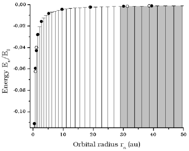
Figure 1: Relationship between energy levels and orbital radii.

V Conclusions

The primary goal of Classical Mechanics is to describe and explain the motion of macroscopic objects affected by external forces. In these systems the observable take continuous values obeying the Principle of stationary action, nonetheless, the quantization of action that just makes certain of this continuum values are permitted. It is clear that Quantum Mechanics can not be applied on a macroscopic scale to the entire physical system, only those where the action is quantized, usually in resonance phenomena or systems where steady states appear.

There are many limitations in a microscopic scale when we want to view or highlight certain theoretical or experimental facts, however, it is possible to create a macroscopic mechanical model that is analogous or equivalent to the microscopic quantum model, obtaining a “toy-model” where we can test some conjectures and observe the behavior and evolution of the system under certain conditions. Although all of the above mentioned has referred just to mechanic systems, it is possible to extend these concepts to the study of another class of physical systems, since in these systems the classical observables quantize or take discrete values too.

- (1) De Broglie, Ondes et mouvements, París, Gauthier-Villars (1926).
- (2) E. Schrödinger, Phys. Rev. 28 (6), 1049–1070 (1926).
- (3) W. Heisenberg, Zeitschrift für Physik 33, 879-893 (1925); M. Born and P. Jordan, Zeitschcrif für Physik 34, 858-888 (1925); M. Born, W. Heisenberg and P. Jordan, Zeits. für Physik 35, 557-615 (1926).
- (4) M. Born. Zeits. für Physik. 37, 893 (1926), Nature 119 354 (1927).
- (5) E. Madelung. Zeits. für Physik A Hadrons and Nuclei, 40, 322–326 (1927).
- (6) D. Bohm. Phys. Rev., 85, 166–179 (1952); Phys. Rev. 85, 180-193 (1952).
- (7) C. L. Lopreore and R. E. Wyatt. Phys. Rev. Lett. 82, 5191–5193 (1999); C. L. Lopreore and R. E. Wyatt. Chem. Phys. Lett. 325, 73–78 (2000); J. B. Maddox and E. R. Bittner. J. Chem. Phys. 119, 6465–6474 (2003); B. K. Kendrik. J. Chem. Phys. 121, 2471–2482 (2004); P. Holland. Anals of Phys. 315, 505–531 (2005).
- (8) M. Arndt et al. Nature 401, 680-682 (1999); O. Nairz, M. Arndt, and A. Zeilinger. Phys. Rev. A 65, 032109 (2002).
- (9) J. R. Friedman et al. Nature 406, 43-46 (2000).
- (10) A. G. Agnese and R. Festa, Phys. Lett. A 227,165 (1997); L. Nottale, G. Schumacher and J. Gay. Astron. Astrophys. 322, 1018–1025 (1997); R. Hermann, G. Schumacher and R. Guyard. Astron. Astrophys. 335, 281–286 (1998); A. Rubĉić and J. Rubĉić. Fizika B 7, 1–13 (1998).
- (11) L. Nottale. Astron. Astrophys. 315, L9-L12 (1996); L. Nottale, G. Schumacher and E.T. Lefèvre. Astron. Astrophys. 361, 379–387 (2000).
- (12) R. Gomes, H. F. Levison, K. Tsiganis and A. Morbidelli. Nature, 435, 466-469 (2005); K. Tsiganis, R. Gomes, A. Morbidelli and H. F. Levison. Nature, 435, 459-461 (2005); A. Morbidelli et al. astro-ph/0706.1713v2.