Abstract

In this paper we relate the matrix ${\mathfrak{S}}_{\cal B}$ of the second moments of a spherically truncated normal multivariate to its full covariance matrix $\Sigma$ and present an algorithm to invert the relation and reconstruct $\Sigma$ from ${\mathfrak{S}}_{\cal B}$. While the eigenvectors of $\Sigma$ are left invariant by the truncation, its eigenvalues are non–uniformly damped. We show that the eigenvalues of $\Sigma$ can be reconstructed from their truncated counterparts via a fixed point iteration, whose convergence we prove analytically. The procedure requires the computation of multidimensional Gaussian integrals over a Euclidean ball, for which we extend a numerical technique, originally proposed by Ruben in 1962, based on a series expansion in chi–square distributions. In order to study the feasibility of our approach, we examine the convergence rate of some iterative schemes on suitably chosen ensembles of Wishart matrices. We finally discuss the practical difficulties arising in sample space and outline a regularization of the problem based on perturbation theory.

1 Introduction

It is more than forty years since Tallis [1] worked out the moment–generating function of a normal multivariate $X\equiv\{X_{k}\}_{k=1}^{v}\,\sim\,{\cal N}_{v}(0,\Sigma)$, subject to the conditional event

$$X\in{\cal E}_{v}(\rho;\Sigma)\,,\qquad\qquad{\cal E}_{v}(\rho;\Sigma)\equiv\,\{x\in{\mathbb{R}}^{v}:\ {x}^{\scriptscriptstyle{\rm T}}\Sigma^{-1}x\leq\rho\}\,.$$ (1.1)

The perfect match between the symmetries of the ellipsoid ${{\cal E}}_{v}(\rho;\Sigma)$ and those of ${\cal N}_{v}(0,\Sigma)$ allows for an exact analytic result, from which the complete set of multivariate truncated moments can be extracted upon differentiation. Consider for instance the matrix ${\mathfrak{S}}_{\cal E}(\rho;\Sigma)$ of the second truncated moments, expressing the covariances among the components of $X$ within ${\cal E}_{v}(\rho;\Sigma)$. From Tallis’ paper it turns out that

$${\mathfrak{S}}_{\cal E}(\rho;\Sigma)=c_{\scriptscriptstyle\rm T}(\rho)\,\Sigma\,,\qquad c_{\scriptscriptstyle\rm T}(\rho)\equiv\,\frac{F_{v+2}(\rho)}{F_{v}(\rho)}\,,$$ (1.2)

with $F_{v}$ denoting the cumulative distribution function of a $\chi^{2}$–variable with $v$ degrees of freedom. Inverting eq. (1.2) – so as to express $\Sigma$ as a function of ${\mathfrak{S}}_{\cal E}$ – is trivial, since $c_{\scriptscriptstyle\rm T}(\rho)$ is a scalar damping factor independent of $\Sigma$. In this paper, we shall refer to such inverse relation as the reconstruction of $\Sigma$ from ${\mathfrak{S}}_{\cal E}$. Unfortunately, life is not always so easy. In general, the effects produced on the expectation of functions of $X$ by cutting off the probability density outside a generic domain ${\cal D}\subset{\mathbb{R}}^{v}$ can be hardly calculated in closed form, especially if the boundary of ${\cal D}$ is shaped in a way that breaks the ellipsoidal symmetry of ${\cal N}_{v}(0,\Sigma)$. Thus, for instance, unlike eq. (1.2) the matrix of the second truncated moments is expected in general to display a non–linear/non–trivial dependence upon $\Sigma$.

In the present paper, we consider the case where ${\cal D}$ is a $v$–dimensional Euclidean ball with center in the origin and square radius $\rho$. Specifically, we discuss the reconstruction of $\Sigma$ from the matrix ${\mathfrak{S}}_{\cal B}$ of the spherically truncated second moments. To this aim, we need to mimic Tallis’ calculation, with eq. (1.1) replaced by the conditional event

$$X\in{\cal B}_{v}(\rho)\,,\qquad\qquad{\cal B}_{v}(\rho)\equiv\,\{x\in{\mathbb{R}}^{v}:\ {x}^{\scriptscriptstyle{\rm T}}x\leq\rho\}\,.$$ (1.3)

This is precisely an example of the situation described in the previous paragraph: although ${\cal B}_{v}(\rho)$ has a higher degree of symmetry than ${\cal E}_{v}(\rho;\Sigma)$, still there is no possibility of obtaining a closed–form relation between $\Sigma$ and ${\mathfrak{S}}_{\cal B}$, since ${\cal B}_{v}(\rho)$ breaks the ellipsoidal symmetry of ${\cal N}_{v}(0,\Sigma)$: technically speaking, in this case we cannot perform any change of variable under the defining integral of the moment–generating function, which may reduce the dimensionality of the problem, as in Tallis’ paper.

In spite of that, the residual symmetries characterizing the truncated distribution help simplify the problem in the following respects: i) the reflection invariance of the whole set–up still yields ${\mathbb{E}}[X_{k}\,|\,X\in{\cal B}_{v}(\rho)]=0$ $\forall\,k$, and ii) the rotational invariance of ${\cal B}_{v}(\rho)$ preserves the possibility of defining the principal components of the distribution just like in the unconstrained case. In particular, the latter property means that ${\mathfrak{S}}_{\cal B}$ and $\Sigma$ share the same orthonormal eigenvectors. In fact, the reconstruction of $\Sigma$ from ${\mathfrak{S}}_{\cal B}$ amounts to solving a system of non–linear integral equations, having the eigenvalues $\lambda\equiv\{\lambda_{k}\}_{k=1}^{v}$ of $\Sigma$ as unknown variables and the eigenvalues $\mu\equiv\{\mu_{k}\}_{k=1}^{v}$ of ${\mathfrak{S}}_{\cal B}$ as input parameters. In a lack of analytic techniques to evaluate exactly the integrals involved, we resort to a numerical algorithm, of which we investigate feasibility, performance and optimization.

The paper is organized as follows. In sect. 2, we describe a couple of examples illustrating the occurrence of spherical truncations in practical situations. In sect. 3, we show that the aforementioned integral equations have the analytic structure of a fixed point vector equation, that is to say $\lambda=T(\lambda)$. This suggests to achieve the reconstruction of $\lambda$ numerically via suitably chosen iterative schemes. In sect. 4, we prove the convergence of the simplest of them by inductive arguments, the validity of which relies upon the monotonicity properties of ratios of Gaussian integrals over ${\cal B}_{v}(\rho)$. In sect. 5, we review some numerical techniques for the computation of Gaussian integrals over ${\cal B}_{v}(\rho)$ with controlled systematic error. These are based on and extend a classic work by Ruben [2] on the distribution of quadratic forms of normal variables. For the sake of readability, we defer proofs of statements made in this sect. to Appendix A. In sect. 6, we report on our numerical experiences: since the simplest iterative scheme, namely the Gauss–Jacobi iteration, is too slow for practical purposes, we investigate the performance of its improved version based on over–relaxation; as expected, we find that the latter has a higher convergence rate, yet it still slows down polynomially in $1/\rho$ as $\rho\to 0$ and exponentially in $v$ as $v\to\infty$; in order to reduce the slowing down, we propose an acceleration technique, which boosts the higher components of the eigenvalue spectrum. A series of Monte Carlo simulations enables us to quantify the speedup. In sect. 7 we discuss the problems arising when $\mu$ is affected by statistical uncertainty and propose a regularization technique based on perturbation theory. To conclude, we summarize our findings in sect. 8.

2 Motivating examples

Spherical truncations of multinormal distributions may characterize different kinds of experimental devices and may occur in various problems of statistical and convex analysis. In this section, we discuss two motivating examples.

2.1 A two–dimensional gedanken experiment in Classical Particle Physics

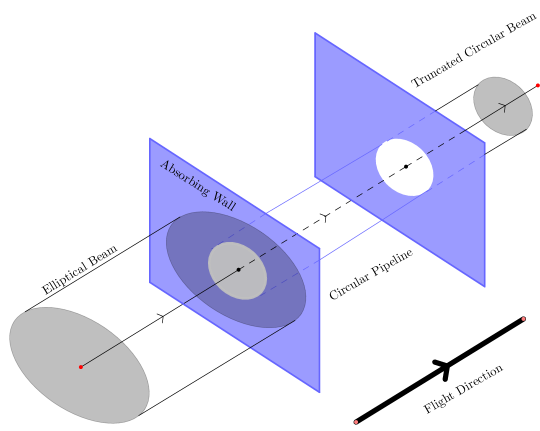
Consider the following ideal situation. An accelerator physicist prepares an elliptical beam of classical particles with Gaussian transversal profile. The experimenter knows a priori the spatial distribution of the beam, i.e. the covariance matrix $\Sigma$ of the two–dimensional coordinates of the particles on a plane orthogonal to their flight direction. We can assume with no loss of generality that the transversal coordinate system has origin at the maximum of the beam intensity and axes along the principal components of the beam, thus it holds $\Sigma={\rm diag}(\lambda_{1},\lambda_{2})$. The beam travels straightforward until it enters a linear coaxial pipeline with circular profile, schematically depicted in Fig. 1, where the beam is longitudinally accelerated. While the outer part of the beam is stopped by an absorbing wall, the inner part propagates within the pipeline. At the end of the beam flight the physicist wants to know if the transversal distribution of the particles is changed, due to unknown disturbance factors arisen within the pipeline. Accordingly, he measures again the spatial covariance matrix of the beam. Unfortunately, the absorbing wall has cut off the Gaussian tail, thus damping the covariance matrix and making it not anymore directly comparable to the original one. To perform such a comparison in the general case $\lambda_{1}\neq\lambda_{2}$, the covariance matrix of the truncated circular beam has to go through the reconstruction procedure described in next sections.

Fig. 1: A classical particle beam with elliptical transversal profile is cut off upon entering a circular coaxial pipeline.

2.2 A multivariate example: connections to Compositional Data Analysis

Compositional Data Analysis (CoDA) has been the subject of a number of papers, pioneered by J. Aitchison [3] over the past forty years. As a methodology of statistical investigation, it finds application in all cases where the main object of interest is a multivariate with strictly positive continuous components to be regarded as portions of a total amount $\kappa$ (the normalization $\kappa=1$ is conventionally adopted in the mathematical literature). In other words, compositional variates belong to the $\kappa$–simplex

$${\cal S}_{v}=\left\{z\in{\mathbb{R}}^{v}_{+}:\quad|z|_{1}=\kappa\right\}\,,\qquad v\geq 2\,,$$ (2.1)

with $|z|_{1}=\sum_{k=1}^{v}z_{k}$ the taxi–cab norm of $z$, while compositions with different norms can be always projected onto ${\cal S}_{v}$ via the closure operator ${\cal C}\cdot x\equiv\{\kappa x_{1}/|x|_{1},\ldots,\kappa x_{v}/|x|_{1}\}$. There are countless types of compositional data, whose analysis raises problems of interest for Statistics [4], e.g. geochemical data, balance sheet data, election data, etc.

In order to measure distances on ${\cal S}_{v}$, Aitchison introduced a positive symmetric function $d_{\rm\scriptscriptstyle A}:{\cal S}_{v}\times{\cal S}_{v}\to{\mathbb{R}}_{+}$, explicitly defined by

$$d_{\rm\scriptscriptstyle A}(x,y)=\sqrt{\frac{1}{2v}\sum_{i,k=1}^{v}\left[\log\left(\frac{x_{i}}{x_{k}}\right)-\log\left(\frac{y_{i}}{y_{k}}\right)\right]^{2}}\,.$$ (2.2)

The Aitchison distance is a key tool in CoDA. It is scale invariant in both its first and second argument, i.e. it is left invariant by redefinitions $z\to\{\alpha z_{1},\ldots,\alpha z_{v}\}$ with $\alpha\in{\mathbb{R}}_{+}$. Accordingly, its support can be extended to ${\mathbb{R}}_{+}^{v}\times{\mathbb{R}}_{+}^{v}$ by imposing

$$d_{\rm\scriptscriptstyle A}(x,y)\equiv d_{\rm\scriptscriptstyle A}({\cal C}\cdot x,{\cal C}\cdot y)\,,\qquad x,y\in{\mathbb{R}}_{+}^{v}\,.$$ (2.3)

It was proved in [5] that $d_{\rm\scriptscriptstyle A}$ is a norm–induced metric on ${\cal S}_{v}$, provided the latter is given an appropriate normed vector space structure. Owing to the compositional constraint $|\cdot|_{1}=\kappa$, it holds $\text{dim}\,{\cal S}_{v}=v-1$. Accordingly, the description of ${\cal S}_{v}$ in terms of $v$ components is redundant: an essential representation requires compositions to be properly mapped onto $(v-1)$–tuples. Among various possibilities, the Isometric Logratio Transform (ILR) introduced in [5], is the only known map of this kind leaving $d_{\rm\scriptscriptstyle A}$ invariant. More precisely, the ILR fulfills

$$d_{\rm\scriptscriptstyle A}(x,y)=d_{\rm\scriptscriptstyle E}\left({\rm ilr}(x),{\rm ilr}(y)\right)\,,\qquad d_{\rm\scriptscriptstyle E}(u,v)\equiv\sqrt{\sum_{k=1}^{v-1}(u_{k}-v_{k})^{2}}\,.$$ (2.4)

It is known from [6] that if $X\sim\log{\cal N}_{v}(\mu,\Sigma)$ is a log–normal $v$–variate, then ${\cal C}\cdot X\sim L_{v}(\mu^{\prime},\Sigma^{\prime})$ is a logistic–normal $v$–variate, with a known relation between $(\mu,\Sigma)$ and $(\mu^{\prime},\Sigma^{\prime})$. Analogously, it is not difficult to show that ${\rm ilr}\left({\cal C}\cdot X\right)\sim{\cal N}_{v-1}(\mu^{\prime\prime},\Sigma^{\prime\prime})$ is a normal $(v-1)$–variate, with $(\mu^{\prime\prime},\Sigma^{\prime\prime})$ related to $(\mu^{\prime},\Sigma^{\prime})$ via the change of basis matrices derived in [5]. Just to sum up, it holds

$$X\sim\log{\cal N}_{v}(\mu,\Sigma)\quad\Rightarrow\quad{\cal C}\cdot X\sim L_{v}(\mu^{\prime},\Sigma^{\prime})\quad\Leftrightarrow\quad{\rm ilr}\left({\cal C}\cdot X\right)\sim{\cal N}_{v-1}(\mu^{\prime\prime},\Sigma^{\prime\prime})\,.$$ (2.5)

Now, suppose that ${\it i})$ $X$ fulfills eq. (2.5) and has a natural interpretation as a composition, ${\it ii})$ a representative set ${\cal D}_{X}$ of observations of $X$ is given and ${\it iii})$ we wish to select from ${\cal D}_{X}$ those units which are compositionally closer to the centre of the distribution, according to the Aitchison distance. To see that the problem is well posed, we first turn ${\cal D}_{X}$ into a set ${\cal D}_{{\cal C}\cdot X}\equiv\{y:y={\cal C}\cdot x\ \text{and}\ x\in{\cal D}_{X}\}$ of compositional observations of $Y={\cal C}\cdot X$. Then, we consider the special point ${\rm cen}[Y]={\cal C}\cdot\exp\{{\mathbb{E}}[\ln Y]\}$, representing the centre of the distribution of $Y$ in a compositional sense: ${\rm cen}[Y]$ minimizes the expression ${\mathbb{E}}[d^{2}_{\rm\scriptscriptstyle A}(Y,{\rm cen}[Y])]$ over ${\cal S}_{v}$ and fulfills ${\rm cen}[Y]={\rm ilr}^{-1}({\mathbb{E}}[{\rm ilr}(Y)])$, see ref. [7]. By virtue of eq. (2.5) this entails ${\rm ilr}({\rm cen}[Y])={\mathbb{E}}[{\rm ilr}(Y)]=\mu^{\prime\prime}$. In order to select the observations which are closer to ${\rm cen}[Y]$, we set a threshold $\delta>0$ and consider only those elements $y\in{\cal D}_{{\cal C}\cdot X}$ fulfilling $d_{\rm\scriptscriptstyle A}^{2}(y,{\rm cen}[y])<\delta$, with ${\rm cen}[y]$ being a sample estimator of ${\rm cen}[Y]$ on ${\cal D}_{{\cal C}\cdot X}$. Such selection rule operates a well–defined truncation of the distribution of $Y$. Moreover, in view of eqs. (2.4) and (2.5), we have

$${\mathbb{P}}\left[d^{2}_{\rm\scriptscriptstyle A}(Y,{\rm cen}[Y])<\delta\ |\ Y\sim L_{v}(\mu^{\prime},\Sigma^{\prime})\right]={\mathbb{P}}\left[d^{2}_{\rm\scriptscriptstyle E}(Z,\mu^{\prime\prime})<\delta\ |\ Z\sim{\cal N}_{v-1}(\mu^{\prime\prime},\Sigma^{\prime\prime})\right]\,,$$ (2.6)

with $Z={\rm ilr}({\cal C}\cdot X)$. As a consequence, we see that a compositional selection rule based on the Aitchison distance and eq. (2.5) is equivalent to a spherical truncation of a multinormal distribution. Obviously, once $Z$ has been spherically truncated, the covariance matrix of the remaining data is damped, thus an estimate of the full covariance matrix requires the reconstruction procedure described in next sections.

2.3 General covariance reconstruction problem

The examples discussed in the previous subsections are special cases of a more general inverse problem, namely the reconstruction of the covariance matrix $\Sigma$ of a normal multivariate $X$ on the basis of the covariance matrix ${\mathfrak{S}}_{\cal D}$ of $X$ truncated to some (convex) region ${\cal D}$. This is the simplest yet non–trivial inverse problem, which can be naturally associated to the normal distribution. The case ${\cal D}={\cal B}_{v}(\rho)$ corresponds to a set–up where theoretical and practical aspects of the problem can be investigated with relatively modest mathematical effort. It is certainly a well–defined framework where to study regularization techniques for non–linear inverse problems in Statistics, for which there is still much room for interesting work [8, 9].

3 Definitions and set–up

Let $X\in{\mathbb{R}}^{v}$ be a random vector with jointly normal distribution ${\cal N}_{v}(0,\Sigma)$ in $v\geq 1$ dimensions. The probability that $X$ falls within ${\cal B}_{v}(\rho)$ is measured by the Gaussian integral

$$\alpha(\rho;\Sigma)\,\equiv\,{\mathbb{P}}\left[X\in{\cal B}_{v}(\rho)\right]\,=\,\frac{1}{(2\pi)^{v/2}|\Sigma|^{1/2}}\int_{{\cal B}_{v}(\rho)}{\rm d}^{v}x\ \exp\left\{-\frac{1}{2}{x}^{\scriptscriptstyle{\rm T}}{\Sigma}^{{-1}}x\right\}\,.$$ (3.1)

Since $\Sigma$ is symmetric positive definite, it has orthonormal eigenvectors $\Sigma v^{(i)}=\lambda_{i}v^{(i)}$. Let us denote by $R\equiv\{v^{(j)}_{i}\}_{i,j=1}^{v}$ the orthogonal matrix having these vectors as columns and by $\Lambda\equiv{\rm diag}(\lambda)={R}^{\scriptscriptstyle{\rm T}}\Sigma R$ the diagonal counterpart of $\Sigma$. From the invariance of ${\cal B}_{v}(\rho)$ under rotations, it follows that $\alpha$ depends upon $\Sigma$ just by way of $\lambda$. Accordingly, we rename the Gaussian probability content of ${\cal B}_{v}(\rho)$ as

$$\alpha(\rho;\lambda)\equiv\int_{{\cal B}_{v}(\rho)}{\rm d}^{v}x\,\prod_{m=1}^{v}\delta(x_{m},\lambda_{m})\,,\qquad\qquad\delta(y,\eta)\,=\,\frac{1}{\sqrt{2\pi\eta}}\exp\left\{-\frac{y^{2}}{2\eta}\right\}\,.$$ (3.2)

Note that eq. (3.2) is not sufficient to fully characterize the random vector $X$ under the spherical constraint, for which we need to calculate the distribution law ${\mathbb{P}}[X\in A|X\in{\cal B}_{v}(\rho)]$ as a function of $A\subset{\mathbb{R}}^{v}$. Alternatively, we can describe $X$ in terms of the complete set of its truncated moments

$$m_{k_{1}\dots k_{v}}(\rho;\Sigma)\,\equiv\,{\mathbb{E}}[X_{1}^{k_{1}}\dots X_{v}^{k_{v}}\,|\,X\in{\cal B}_{v}(\rho)]\,,\qquad\{k_{i}\}_{i=1,\ldots,v}\in{\mathbb{N}}^{v}\,,$$ (3.3)

As usual, these can be all obtained from the moment–generating function

$$\alpha\,m(t)=\,\frac{1}{(2\pi)^{v/2}|\Sigma|^{1/2}}\int_{{\cal B}_{v}(\rho)}{\rm d}^{v}x\,\exp\left\{{t}^{\scriptscriptstyle{\rm T}}x-\frac{1}{2}{x}^{\scriptscriptstyle{\rm T}}{\Sigma}^{{-1}}x\right\}\,,\qquad t\in{\mathbb{R}}^{v}\,,$$ (3.4)

by differentiating the latter an arbitrary number of times with respect to the components of $t$, viz.

$$m_{k_{1}\dots k_{v}}(\rho;\Sigma)=\,\frac{\partial^{\,k_{1}+\ldots+k_{v}}\,m(t)}{(\partial t_{1})^{k_{1}}\dots(\partial t_{v})^{k_{v}}}\biggr{|}_{t=0}\,.$$ (3.5)

It will be observed that $m(t)$ is in general not invariant under rotations of $t$. Therefore, unlike $\alpha$, the moments $m_{k_{1}\ldots k_{v}}$ depend effectively on both $\lambda$ and $R$. For instance, for the matrix of the second moments ${\mathfrak{S}}_{\cal B}\equiv\{\partial^{2}m/\partial t_{i}\partial t_{j}|_{t=0}\}_{i,j=1}^{v}$ such dependence amounts to

$$\alpha\,({{\mathfrak{S}}_{\cal B}})_{ij}\,=\,\sum_{k,\ell=1}^{v}R_{ki}R_{\ell j}\int_{{\cal B}_{v}(\rho)}{\rm d}^{v}x\ x_{k}x_{\ell}\,\prod_{m=1}^{v}\delta(x_{m},\lambda_{m})\,.$$ (3.6)

By parity, the only non–vanishing terms in the above sum are those with $k=\ell$. Hence, it follows that $\Sigma$ and ${\mathfrak{S}}_{\cal B}$ share $R$ as a common diagonalizing matrix. In other words, if $M\equiv{\rm diag}(\mu)$ is the diagonal matrix of the eigenvalues of ${\mathfrak{S}}_{\cal B}$, then $M={R}^{\scriptscriptstyle{\rm T}}{\mathfrak{S}}_{\cal B}R$. Moreover, $\mu_{k}$ is related to $\lambda_{k}$ by

$$\mu_{k}=\lambda_{k}\frac{\alpha_{k}}{\alpha}\,,\qquad\qquad\alpha_{k}(\rho;\lambda)\equiv\int_{{\cal B}_{v}(\rho)}{\rm d}^{v}x\ \frac{x_{k}^{2}}{\lambda_{k}}\,\prod_{m=1}^{v}\delta(x_{m},\lambda_{m})\,,\qquad k=1,\ldots,v\,.$$ (3.7)

The ratios $\alpha_{k}/\alpha$ are naturally interpreted as adimensional correction factors to the eigenvalues of $\Sigma$, so they play the same rôle as $c_{\scriptscriptstyle\rm T}(\rho)$ in eq. (1.2). However, $\alpha_{k}/\alpha$ depends explicitly on the subscript $k$, thus each eigenvalue is damped differently from the others as a consequence of the condition $X\in{\cal B}_{v}(\rho)$.

Remark 3.1.

In practical terms, eqs. (3.6)–(3.7) tell us that estimating the sample covariance matrix of $X\sim{\cal N}_{v}(0,\Sigma)$ from a spherically truncated population $\{x^{(m)}\}_{m=1}^{M}$, made of $M$ independent units, via the classical estimator $Q_{ij}=(M-1)^{-1}\sum_{m=1}^{M}(x_{i}^{(m)}-{\tilde{x}}^{(m)}_{i})(x_{j}^{(m)}-{\tilde{x}}^{(m)}_{j})$, being $\tilde{x}=M^{-1}\sum_{m=1}^{M}x^{(m)}$ the sample mean, yields a damped result. Nonetheless, the damping affects only the eigenvalues of the estimator, whereas its eigenvectors are left invariant.

3.1 Montonicity properties of ratios of Gaussian integrals

Eqs. (3.2) and (3.7) suggest to introduce a general notation for the Gaussian integrals over ${\cal B}_{v}(\rho)$, under the assumption $\Sigma=\Lambda$. So, we define

$$\alpha_{k\ell m\dots}(\rho;\lambda)\equiv\int_{{\cal B}_{v}(\rho)}{\rm d}^{v}x\ \frac{x_{k}^{2}}{\lambda_{k}}\,\frac{x_{\ell}^{2}}{\lambda_{\ell}}\,\frac{x_{m}^{2}}{\lambda_{m}}\dots\,\prod_{n=1}^{v}\delta(x_{n},\lambda_{n})\,,$$ (3.8)

with each subscript $q$ on the l.h.s. addressing an additional factor of $x_{q}^{2}/\lambda_{q}$ under the integral sign on the r.h.s. (no subscripts means $\alpha$). Several analytic properties of such integrals are discussed in ref. [10]. Here, we lay emphasis on some issues concerning the monotonicity trends of the ratios $\alpha_{k}/\alpha$. Specifically,

Proposition 3.1 (monotonicities).

Let $\lambda_{(k)}\equiv\{\lambda_{i}\}_{i=1,\ldots,v}^{i\neq k}$ denote the set of the full eigenvalues without $\lambda_{k}$. The ratios $\alpha_{k}/\alpha$ fulfill the following properties:

• $\lambda_{k}\dfrac{\alpha_{k}}{\alpha}(\rho;\lambda)$ is a monotonic increasing function of $\lambda_{k}$ at fixed $\rho$ and $\lambda_{(k)}$;

• $\dfrac{\alpha_{k}}{\alpha}(\rho;\lambda)$ is a monotonic decreasing function of $\lambda_{k}$ at fixed $\rho$ and $\lambda_{(k)}$;

• $\dfrac{\alpha_{k}}{\alpha}(\rho;\lambda)$ is a monotonic decreasing function of $\lambda_{i}$ $(i\neq k)$ at fixed $\rho$ and $\lambda_{(i)}$,

where an innocuous abuse of notation has been made on writing $\frac{\alpha_{k}}{\alpha}(\rho;\lambda)$ in place of $\alpha_{k}(\rho;\lambda)/\alpha(\rho;\lambda)$.

Proof.

Let the symbol $\partial_{k}\equiv\partial/\partial\lambda_{k}$ denote a derivative with respect to $\lambda_{k}$. In order to prove property $p_{1}$), we apply the chain rule of differentiation to $\lambda_{k}\alpha_{k}/\alpha$ and then we pass $\partial_{k}$ under the integral sign in $\partial_{k}\alpha$ and $\partial_{k}\alpha_{k}$. In this way, we obtain

$$\partial_{k}\left(\lambda_{k}\frac{\alpha_{k}}{\alpha}\right) =\ \frac{1}{2}\left(\frac{\alpha_{kk}}{\alpha}-\frac{\alpha_{k}^{2}}{\alpha^{2}}\right)=\frac{1}{2\lambda_{k}^{2}}\left\{{\mathbb{E}}[X_{k}^{4}\,|\,X\in{\cal B}_{v}(\rho)]-{\mathbb{E}}[X_{k}^{2}\,|\,X\in{\cal B}_{v}(\rho)]^{2}\right\}$$

$$=\ \frac{1}{2\lambda_{k}^{2}}{\rm var}\left(X_{k}^{2}\,|\,X\in{\cal B}_{v}(\rho)\right)\geq 0\,.$$ (3.9)

Moreover, since the truncated marginal density of $X_{k}^{2}$ is positive within a set of non–zero measure in ${\mathbb{R}}$, the monotonic trend of $\lambda_{k}\alpha_{k}/\alpha$ in $\lambda_{k}$ is strict. $\boxdot$ Properties $p_{2}$) and $p_{3}$) are less trivial than $p_{1}$). Indeed, the same reasoning as above now yields on the one hand

$$\lambda_{k}\partial_{k}\left(\frac{\alpha_{k}}{\alpha}\right) =\partial_{k}\left(\lambda_{k}\frac{\alpha_{k}}{\alpha}\right)-\frac{\alpha_{k}}{\alpha}$$

$$=\frac{1}{2\lambda_{k}^{2}}\left\{{\rm var}\left(X_{k}^{2}\,|\,X\in{\cal B}_{v}(\rho)\right)-2\lambda_{k}{\mathbb{E}}[X_{k}^{2}\,|\,X\in{\cal B}_{v}(\rho)]\right\}\leq 0\,,$$ (3.10)

and on the other

$$\hskip 2.84544pt\lambda_{i}\partial_{i}\left(\frac{\alpha_{k}}{\alpha}\right)=\frac{1}{2}\left(\frac{\alpha_{ik}}{\alpha}-\frac{\alpha_{i}\alpha_{k}}{\alpha^{2}}\right)=\frac{1}{2\lambda_{i}\lambda_{k}}{\rm cov}\left(X_{i}^{2},X_{k}^{2}\,|\,X\in{\cal B}_{v}(\rho)\right)\leq 0\,\qquad(i\neq k)\,.$$ (3.11)

Though not a priori evident, the r.h.s. of both eqs. (3.10) and (3.11) is negative (and vanishes in the limit $\rho\to\infty$). The inequalities ${\rm var}(X_{k}^{2})\leq 2\lambda_{k}{\mathbb{E}}[X_{k}^{2}]$ within Euclidean balls have been first discussed in [10], while the inequalities ${\rm cov}(X_{j}^{2},X_{k}^{2})$ within generalized Orlicz balls have been discussed in refs. [11, 12] for the case where the probability distribution of $X$ is flat instead of being normal. More recently, a complete proof of both inequalities has been given in [13]. Despite the technical difficulties in proving them, their meaning should be intuitively clear. The variance inequality quantifies the squeezing affecting $X_{k}^{2}$ as a consequence of the truncation (in the unconstrained case it would be ${\rm var}(X_{k}^{2})=2\lambda_{k}^{2}$). The covariance inequality follows from the opposition arising among the square components in proximity of the boundary of ${\cal B}_{v}(\rho)$. Indeed, if $X_{j}^{2}\nearrow\rho$, then $X^{2}_{k}\searrow 0$ $\forall\,k\neq j$ in order for $X$ to stay within ${\cal B}_{v}(\rho)$. ∎

3.2 Definition domain of the reconstruction problem

A consequence of Proposition 3.1 is represented by the following

Corollary 3.1.

Given $v$, $\rho$ and $\lambda$, $\mu_{k}$ is bounded by

$$\frac{\rho}{r\left(v,\frac{\rho}{2\lambda_{k}}\right)}\leq\,\mu_{k}\,\leq\frac{\rho}{3}\,,\qquad\qquad r(v,z)\equiv(2v+1)\dfrac{M\left(v,v+{1}/{2},z\right)}{M\left(v,v+{3}/{2},z\right)}\,,$$ (3.12)

with $M$ denoting the Kummer function, viz.

$$M(a,b,z)=\sum_{n=0}^{\infty}\frac{1}{n!}\frac{(a)_{n}}{(b)_{n}}\,z^{n}\,,\qquad(x)_{n}\equiv\frac{\Gamma(x+n)}{\Gamma(x)}\,.$$ (3.13)

Proof.

The upper bound of eq. (3.12) corresponds to the value of $\mu_{k}$ in the $v$–tuple limit $\lambda_{k}\to\infty$, $\lambda_{(k)}\to\{0\,\ldots,0\}$. This is indeed the maximum possible value allowed for $\mu_{k}$ according to properties $p_{1}$) and $p_{3}$) of Proposition 3.1. In order to perform this limit, we observe that

$$\lim_{\eta\to 0^{+}}\delta(y,\eta)=\delta(y)\,,$$ (3.14)

with the $\delta$ symbol on the r.h.s. representing the Dirac delta function (the reader who is not familiar with the theory of distributions may refer for instance to ref. [14] for an introduction). Accordingly,

$$\lim_{\lambda_{k}\to\infty}\,\lim_{\lambda_{(k)}\to\{0,\ldots,0\}}\,\mu_{k}\ =\ {\displaystyle{\int_{-\sqrt{\rho}}^{+\sqrt{\rho}}{\rm d}x_{k}\ x_{k}^{2}}}\biggl{/}{\displaystyle{\int_{-\sqrt{\rho}}^{+\sqrt{\rho}}{\rm d}x_{k}}}=\frac{\rho}{3}\,.$$ (3.15)

The lower bound corresponds instead to the value taken by $\mu_{k}$ as $\lambda_{(k)}\to\{\infty\,\ldots,\infty\}$ and $\lambda_{k}$ is kept fixed. In this limit, all the Gaussian factors in the probability density function except the $k^{\rm th}$ one flatten to one. Hence,

$$\lim_{\lambda_{(k)}\to\{\infty\,\ldots,\infty\}}\mu_{k}\ =\lim_{\lambda_{(k)}\to\{\infty\,\ldots,\infty\}}\frac{\displaystyle{\int_{-\sqrt{\rho}}^{+\sqrt{\rho}}{\rm d}x_{k}\,x_{k}^{2}\,\delta(x_{k},\lambda_{k})\ \alpha^{(v-1)}\left(\rho-x_{k}^{2};\lambda_{(k)}\right)}}{\displaystyle{\int_{-\sqrt{\rho}}^{+\sqrt{\rho}}{\rm d}x_{k}\ \delta(x_{k},\lambda_{k})\ \alpha^{(v-1)}\left(\rho-x_{k}^{2};\lambda_{(k)}\right)}}$$

$$\hskip 28.45274pt=\frac{\displaystyle{\int_{-\sqrt{\rho}}^{+\sqrt{\rho}}{\rm d}x_{k}\,x_{k}^{2}\,{\rm e}^{-\frac{x_{k}^{2}}{2\lambda_{k}}}\,\left(\rho-x_{k}^{2}\right)^{v-1}}}{\displaystyle{\int_{-\sqrt{\rho}}^{+\sqrt{\rho}}{\rm d}x_{k}\ {\rm e}^{-\frac{x_{k}^{2}}{2\lambda_{k}}}\,\left(\rho-x_{k}^{2}\right)^{v-1}}}=\rho\frac{\displaystyle{\int_{0}^{1}{\rm d}x_{k}\,x_{k}^{2}\,{\rm e}^{-\frac{\rho}{2\lambda_{k}}x_{k}^{2}}\,\left(1-x_{k}^{2}\right)^{v-1}}}{\displaystyle{\int_{0}^{1}{\rm d}x_{k}\ {\rm e}^{-\frac{\rho}{2\lambda_{k}}x_{k}^{2}}\,\left(1-x_{k}^{2}\right)^{v-1}}}\,.$$ (3.16)

Numerator and denominator of the rightmost ratio are easily recognized to be integral representations of Kummer functions (see e.g. ref. [15, ch. 13]). ∎

The upper bound of eq. (3.12) can be sharpened, as clarified by the following

Proposition 3.2 (Bounds on the truncated moments).

Let $v$, $\rho$ and $\lambda$ be given. If $\{i_{1},\ldots,i_{v}\}$ is a permutation of $\{1,\ldots,v\}$ such that $\mu_{i_{1}}\leq\mu_{i_{2}}\leq\ldots\leq\mu_{i_{v}}$, then the following upper bounds hold:

$$i)\quad\sum_{k=1}^{v}\mu_{k}\ \leq\ \rho\,;\qquad\qquad ii)\quad\mu_{i_{k}}\ \leq\ \frac{\rho}{v-k+1}\,,\quad k=1,\ldots,v\,.$$ (3.17)

Proof.

The overall upper bound on the sum of truncated moments follows from

$$\sum_{k=1}^{v}\mu_{k}\ =\ \frac{1}{\alpha}\sum_{k=1}^{v}\lambda_{k}\alpha_{k}\ =\ \frac{1}{\alpha}\int_{{\cal B}_{v}(\rho)}{\rm d}^{v}x\ \left(\sum_{k=1}^{v}x_{k}^{2}\right)\,\prod_{m=1}^{v}\delta(x_{m},\lambda_{m})\,\leq\rho\,.$$ (3.18)

At the same time, the sum can be split and bounded from below by

$$\sum_{k=1}^{v}\mu_{i_{k}}\ =\ \sum_{k=1}^{n}\mu_{i_{k}}+\sum_{k=n+1}^{v}\mu_{i_{k}}\ \geq\ \sum_{k=1}^{n}\mu_{i_{k}}+(v-n)\mu_{i_{n+1}}\,,\qquad n=0,1,\ldots,v-1\,.$$ (3.19)

The single upper bounds on the $\mu_{k}$’s are then obtained from eqs. (3.18)–(3.19). It will be noted that eq. (3.17) ii) is sharper than the upper bound of eq. (3.12) only for $v>3$ and $k<v-2$. ∎

From now on, we shall assume with no loss of generality, that the eigenvalues of $\Sigma$ are increasingly ordered, namely $0<\lambda_{1}\leq\dots\leq\lambda_{v}$ (we can always permute the labels of the coordinate axes, so as to let this be the case). An important aspect related to the eigenvalue ordering is provided by the following

Proposition 3.3 (Eigenvalue ordering).

Let $v$, $\rho$ and $\lambda$ be given. If $\lambda_{1}\leq\lambda_{2}\leq\ldots\leq\lambda_{v}$, then it holds $\mu_{1}\leq\mu_{2}\leq\ldots\leq\mu_{v}$ as well.

Proof.

In order to show that the spherical truncation does not violate the eigenvalue ordering, we make repeated use of the monotonicity properties of Proposition 3.1. Specifically, if $i<j$ then

$$\mu_{i} \ =\,\lambda_{i}\frac{\alpha_{i}}{\alpha}(\rho;\{\lambda_{1},\ldots,\lambda_{i},\ldots,\lambda_{j},\ldots,\lambda_{v}\})$$

$$\ \leq\,\lambda_{j}\frac{\alpha_{i}}{\alpha}(\rho;\{\lambda_{1},\ldots,\lambda_{j},\ldots,\lambda_{j},\ldots,\lambda_{v}\})\quad\quad\hskip 0.86108pt\color[rgb]{0,0,0}\definecolor[named]{pgfstrokecolor}{rgb}{0,0,0}{\leftrightsquigarrow}\quad\text{increasing monotonicity of }\lambda_{i}\frac{\alpha_{i}}{\alpha}$$

$$\ =\,\lambda_{j}\frac{\alpha_{j}}{\alpha}(\rho;\{\lambda_{1},\ldots,\lambda_{j},\ldots,\lambda_{j},\ldots,\lambda_{v}\})\quad\quad\color[rgb]{0,0,0}\definecolor[named]{pgfstrokecolor}{rgb}{0,0,0}{\leftrightsquigarrow}\quad\text{exchange symmetry }i\leftrightarrow j$$

$$\ \leq\,\lambda_{j}\frac{\alpha_{j}}{\alpha}(\rho;\{\lambda_{1},\ldots,\lambda_{i},\ldots,\lambda_{j},\ldots,\lambda_{v}\})\quad\quad\hskip 0.4736pt\color[rgb]{0,0,0}\definecolor[named]{pgfstrokecolor}{rgb}{0,0,0}{\leftrightsquigarrow}\quad\text{decreasing monotonicity of }\frac{\alpha_{j}}{\alpha}$$

$$\ =\,\mu_{j}\,,$$ (3.20)

where the symbol “$\leftrightsquigarrow$” is used to explain where the inequality sign preceding it comes from, and the “exchange symmetry” refers to the formal property of the one–index Gaussian integrals over ${\cal B}_{v}(\rho)$ to fulfill $\alpha_{i}(\rho;\{\lambda_{1},\ldots,\lambda_{i},\ldots,\lambda_{j},\ldots,\lambda_{v}\})=\alpha_{j}(\rho;\{\lambda_{1},\ldots,\lambda_{j},\ldots,\lambda_{i},\ldots,\lambda_{v}\})$. ∎

Let us now focus on eqs. (3.7). They have to be solved in order to reconstruct $\lambda$ from $\mu$. Formally, if we introduce a family of truncation operators $\tau_{\rho}:{\mathbb{R}}^{v}_{+}\to{\mathbb{R}}^{v}_{+}$ (parametrically depending on $\rho$), such that

$$(\tau_{\rho}\cdot\lambda)_{k}\ \equiv\ \lambda_{k}\frac{\alpha_{k}}{\alpha}(\rho;\lambda)\,,\qquad k=1,\dots,v\,,$$ (3.21)

then the reconstruction of $\lambda$ from $\mu$ amounts to calculating $\lambda=\tau_{\rho}^{-1}\cdot\mu$. One should be aware that $\tau_{\rho}$ is not a surjective operator in view of Corollary 3.1 and Proposition 3.2. Therefore, $\tau_{\rho}^{-1}$ is only defined within a bounded domain ${\cal D}(\tau_{\rho}^{-1})$. If we define

$${\cal D}_{0} =\left\{\mu\in{\mathbb{R}}^{v}_{+}:\quad\mu_{1}\leq\ldots\leq\mu_{v}\ \text{ and }\right.$$

$$\hskip 72.55461pt\left.\mu_{k}=\lambda_{k}\frac{\alpha_{k}}{\alpha}\ \text{ for }\ k=1,\ldots,v\ \text{ and for some }\lambda\in{\mathbb{R}}^{v}_{+}\right\}\,,$$ (3.22)

then we have ${\cal D}(\tau_{\rho}^{-1})=\{\mu:\mu=\sigma\cdot\mu_{0}\text{ for some }\mu_{0}\in{\cal D}_{0}\text{ and }\sigma\in S_{v}\}$, where $S_{v}$ is the set of permutations of $v$ elements. From Proposition 3.2 we conclude ${\cal D}_{0}\subseteq H_{v}(\rho)$, being

$$H_{v}(\rho)\ \equiv\ \left\{x\in{\mathbb{R}}^{v}_{+}:\ x_{k}\,\leq\,\min\left\{\frac{\rho}{3},\frac{\rho}{v-k+1}\right\}\ \text{ and }\ \sum_{k=1}^{v}x_{k}\leq\rho\,,\quad\forall\ k\right\}\,.$$ (3.23)

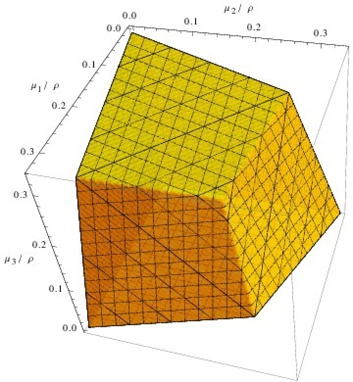
In fact, there are vectors $\mu\in{\mathbb{R}}^{v}_{+}$ fulfilling $\mu\in H_{v}(\rho)$ and $\mu\notin{\cal D}_{0}$, thus we conclude that ${\cal D}_{0}$ is a proper subset of $H_{v}(\rho)$. Numerical experiences based on the techniques discussed in the next sections show indeed that

$${\cal D}(\tau_{\rho}^{-1})=\bigcap_{k=1}^{v}\biggl{\{}\,\mu\in{\mathbb{R}}^{v}_{+}:\quad\sum_{j\neq k}^{1\ldots v}\mu_{j}+3\mu_{k}\leq\rho\,\biggr{\}}\,.$$ (3.24)

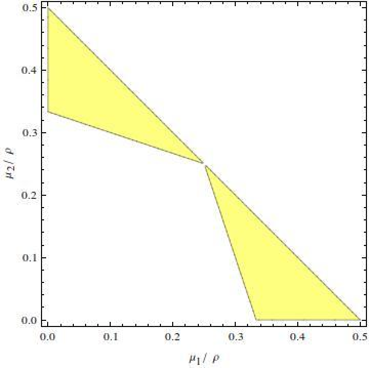
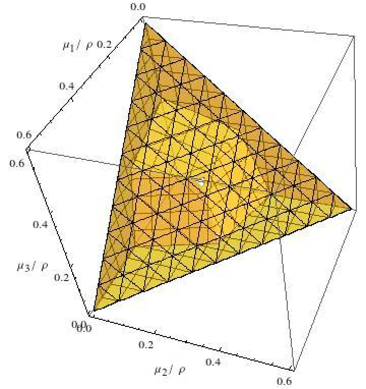
A graphical representation of eq. (3.24) in $v=2$ and $v=3$ dimensions is depicted in Fig. 2. The reader should note that until sect. 7 we shall always assume that $\mu$ comes from the application of $\tau_{\rho}$ to some $\lambda$, thus $\mu\in{\cal D}(\tau_{\rho}^{-1})$ by construction.

         a

Fig. 2: Left: Numerical reconstruction of ${\cal D}(\tau_{\rho}^{-1})$ in $v=2$ dimensions. Right: Numerical reconstruction of ${\cal D}(\tau_{\rho}^{-1})$ in $v=3$ dimensions.

Now, we observe that eqs. (3.7) can be written in the equivalent form

$$\lambda=T(\lambda;\mu;\rho)\,,$$ (3.25)

$$T:\ {\mathbb{R}}^{v}_{+}\times{\mathbb{R}}^{v}_{+}\times{\mathbb{R}}_{+}\,\to\,{\mathbb{R}}^{v}_{+}\,;\qquad T_{k}(\lambda;\mu;\rho)=\mu_{k}\frac{\alpha}{\alpha_{k}}(\rho;\lambda)\,,\qquad k=1,\dots,v\,.$$ (3.26)

Since $\rho$ and $\mu$ are (non–independent) input parameters for the covariance reconstruction problem (and in order to keep the notation light), in the sequel we shall leave the dependence of $T$ upon $\rho$ and $\mu$ implicitly understood, i.e., we shall write eq. (3.25) as $\lambda=T(\lambda)$. Hence, we see that the full eigenvalue spectrum $\lambda$ is a fixed point of the operator $T$. This suggests to obtain it as the limit of a sequence

$$\lambda^{(0)}=\,\mu\,,\qquad\lambda^{(n+1)}\,=\,T(\lambda^{(n)})\,,\qquad n=0,1,\dots\,,$$ (3.27)

$$\lambda\,=\,\lim_{n\to\infty}\lambda^{(n)}\,,$$ (3.28)

provided this can be shown to converge. Note that since $\alpha_{k}<\alpha$, it follows that $T_{k}(\lambda^{(n)})>\mu_{k}$ $\forall n$, so the sequence is bounded from below by $\mu$. In particular, this holds for $n=0$. Therefore, the sequence moves to the right direction at least at the beginning. A formal proof of convergence, based on the monotonicity properties stated by Proposition 3.1, is given in next section.

4 Convergence of the fixed point equation

We split our argument into three propositions, describing different properties of the sequence $\lambda^{(n)}$. They assert respectively that i) the sequence is component–wise monotonic increasing; ii) the sequence is component–wise bounded from above by any fixed point of $T$; iii) if $T$ has a fixed point, this must be unique. Statements i) and ii) are sufficient to guarantee the convergence of the sequence to a finite limit (the unconstrained spectrum is a fixed point of $T$). In addition, the limit is easily recognized to be a fixed point of $T$. Hence, statement iii) guarantees that the sequence converges to the unconstrained eigenvalue spectrum. We remark that all the monotonicities discussed in Proposition 3.1 are strict, i.e. the ratios $\alpha_{k}/\alpha$ have no stationary points at finite $\rho$ and $\lambda$, which is crucial for the proof.

Proposition 4.1 (Increasing monotonicity).

Given $v$, $\rho$ and $\mu\in{\cal D}(\tau_{\rho}^{-1})$, the sequence $\lambda^{(0)}=\mu$, $\lambda^{(n+1)}=T(\lambda^{(n)})$, $n=0,1,\ldots$ is monotonic increasing, viz. $\lambda_{k}^{(n+1)}>\lambda_{k}^{(n)}$  $\forall\,k=1,\ldots,v$.

Proof.

The proof is by induction. We first notice that

$$\lambda_{k}^{(1)}=T_{k}(\lambda^{(0)})=T_{k}(\mu)=\mu_{k}\frac{\alpha}{\alpha_{k}}(\rho;\mu)>\mu_{k}=\lambda_{k}^{(0)}\,,\qquad k=1,\ldots,v\,,$$ (4.1)

the inequality following from $\alpha_{k}(\rho;\mu)<\alpha(\rho;\mu)$. Suppose now that the property of increasing monotonicity has been checked off up to the $n^{\rm th}$ element of the sequence. Then,

$$\lambda_{k}^{(n+1)}=\mu_{k}\frac{\alpha}{\alpha_{k}}(\rho;\lambda^{(n)})>\mu_{k}\frac{\alpha}{\alpha_{k}}(\rho;\lambda^{(n-1)})=\lambda_{k}^{(n)}\,,$$ (4.2)

the inequality following this time from the inductive hypothesis and from properties $p_{2}$) and $p_{3}$) of Proposition 3.1. ∎

Proposition 4.2 (Boundedness).

Given $v$, $\rho$ and $\mu\in{\cal D}(\tau_{\rho}^{-1})$, the sequence $\lambda^{(0)}=\mu$, $\lambda^{(n+1)}=T(\lambda^{(n)})$, $n=0,1,\ldots$ is bounded from above, viz. $\lambda_{k}^{(n)}<\lambda_{k}^{*}$  $\forall\,k=1,\ldots,v$, being $\lambda^{*}$ a fixed point of $T$.

Proof.

We proceed again by induction. We first notice that

$$\lambda_{k}^{(0)}=\mu_{k}<\mu_{k}\frac{\alpha}{\alpha_{k}}(\rho;\lambda^{*})=\lambda_{k}^{*}\,,\qquad k=1,\ldots,v\,,$$ (4.3)

the inequality following as previously from $\alpha_{k}(\rho;\lambda^{*})<\alpha(\rho;\lambda^{*})$. Suppose now that the property of boundedness has been checked off up to the $n^{\rm th}$ element of the sequence. Then,

$$\lambda_{k}^{(n+1)}=\mu_{k}\frac{\alpha}{\alpha_{k}}(\rho;\lambda^{(n)})=\lambda_{k}^{*}\frac{\alpha_{k}}{\alpha}(\rho;\lambda^{*})\frac{\alpha}{\alpha_{k}}(\rho;\lambda^{(n)})<\lambda_{k}^{*}\frac{\alpha_{k}}{\alpha}(\rho;\lambda^{(n)})\frac{\alpha}{\alpha_{k}}(\rho;\lambda^{(n)})=\lambda_{k}^{*}\,,$$ (4.4)

the inequality following for the last time from the inductive hypothesis and from properties $p_{2}$) and $p_{3}$) of Proposition 3.1. ∎

According to Propositions 4.1 and 4.2, the sequence converges. Now, let $\tilde{\lambda}=\lim_{n\to\infty}\,\lambda^{(n)}$ be the limit of the sequence. Effortlessly, we prove that $\tilde{\lambda}$ is a fixed point of $T$. Indeed,

$$\tilde{\lambda}_{k}\,=\,\lim_{n\to\infty}\lambda_{k}^{(n)}\,=\,\lim_{n\to\infty}\mu_{k}\frac{\alpha}{\alpha_{k}}(\rho;\lambda^{(n-1)})\,=\,\mu_{k}\frac{\alpha}{\alpha_{k}}\left(\rho;\lim_{n\to\infty}\lambda^{(n-1)}\right)\,=\,T_{k}(\tilde{\lambda})\,.$$ (4.5)

Note that passing the limit over $n$ under the integral sign is certainly allowed for Gaussian integrals.

Proposition 4.3 (Uniqueness of the fixed point).

Let $\lambda^{\prime}=T(\lambda^{\prime})$ and $\lambda^{\prime\prime}=T(\lambda^{\prime\prime})$ be two fixed points of $T$, corresponding to the same choice of $v$, $\rho$ and $\mu\in{\cal D}(\tau_{\rho}^{-1})$. Then, it must be $\lambda^{\prime}=\lambda^{\prime\prime}$.

Proof.

According to the hypothesis, $\lambda^{\prime}$ and $\lambda^{\prime\prime}$ fulfill the equations

$$\lambda^{\prime}_{k} =\mu_{k}\frac{\alpha}{\alpha_{k}}(\rho;\lambda^{\prime})\qquad\hskip 2.15277pt\Rightarrow\qquad\mu_{k}=\lambda^{\prime}_{k}\frac{\alpha_{k}}{\alpha}(\rho;\lambda^{\prime})\,,$$ (4.6)

$$\lambda^{\prime\prime}_{k} =\mu_{k}\frac{\alpha}{\alpha_{k}}(\rho;\lambda^{\prime\prime})\qquad\Rightarrow\qquad\mu_{k}=\lambda^{\prime\prime}_{k}\frac{\alpha_{k}}{\alpha}(\rho;\lambda^{\prime\prime})\,.$$ (4.7)

Hence,

$$0=\mu_{k}-\mu_{k}=\lambda^{\prime}_{k}\frac{\alpha_{k}}{\alpha}(\rho;\lambda^{\prime})-\lambda_{k}^{\prime\prime}\frac{\alpha_{k}}{\alpha}(\rho;\lambda^{\prime\prime})=\sum_{\ell=1}^{v}\left[\int_{0}^{1}{\rm d}t\ J_{k\ell}\left(\rho;\lambda^{\prime\prime}+t\left(\lambda^{\prime}-\lambda^{\prime\prime}\right)\right)\right](\lambda^{\prime}_{\ell}-\lambda^{\prime\prime}_{\ell})\,,$$ (4.8)

where $J$ denotes the Jacobian matrix of $\tau_{\rho}$ and is given by

$$J_{k\ell}(\rho;\lambda)=\partial_{k}\left(\lambda_{\ell}\frac{\alpha_{\ell}}{\alpha}(\rho;\lambda)\right)=\frac{1}{2}\frac{\lambda_{\ell}}{\lambda_{k}}\left(\frac{\alpha_{k\ell}}{\alpha}-\frac{\alpha_{k}\alpha_{\ell}}{\alpha^{2}}\right)=\left[\Lambda^{-1}\,\Omega(\rho;\lambda)\,\Lambda\right]_{k\ell}\,,$$ (4.9)

having set $\Omega_{k\ell}\equiv(1/2)(\alpha_{k\ell}/\alpha-\alpha_{k}\alpha_{\ell}/\alpha^{2})$. It will be noted that $\Omega=\{\Omega_{k\ell}\}_{k,\ell=1}^{v}$ is essentially the covariance matrix of the square components of $X$ under spherical truncation (we have come across its matrix elements in eqs. (3.9)–(3.11)). As such, $\Omega$ is symmetric positive definite. Indeed,

$$\Omega_{k\ell} =\,\frac{1}{2\lambda_{k}\lambda_{\ell}}{\rm cov}\left(X_{k}^{2},X_{\ell}^{2}\,|\,X\in{\cal B}_{v}(\rho)\right)$$

$$=\,\frac{1}{2\lambda_{k}\lambda_{\ell}}{\mathbb{E}}\biggl{[}\biggl{(}X_{k}^{2}-{\mathbb{E}}\left[X_{k}^{2}\,|\,X\in{\cal B}_{v}(\rho)\right]\biggr{)}\biggl{(}X_{\ell}^{2}-{\mathbb{E}}[X_{\ell}^{2}\,|\,X\in{\cal B}_{v}(\rho)]\biggr{)}\,\biggr{|}\,X\in{\cal B}_{v}(\rho)\biggr{]}\,.$$ (4.10)

On setting $Z_{k}=(X_{k}^{2}-{\mathbb{E}}[X_{k}^{2}\,|\,X\in{\cal B}_{v}(\rho)])/\sqrt{2}\lambda_{k}$, we can represent $\Omega$ as $\Omega={\mathbb{E}}[Z{Z}^{\scriptscriptstyle{\rm T}}\,|\,X\in{\cal B}_{v}(\rho)]$. If $x\in{\mathbb{R}}^{v}$ is not the null vector, then ${x}^{\scriptscriptstyle{\rm T}}\Omega x={\mathbb{E}}[{x}^{\scriptscriptstyle{\rm T}}Z{Z}^{\scriptscriptstyle{\rm T}}x\,|\,X\in{\cal B}_{v}(\rho)]={\mathbb{E}}[({x}^{\scriptscriptstyle{\rm T}}Z)^{2}\,|\,X\in{\cal B}_{v}(\rho)]>0$. Moreover, the eigenvalues of $\Omega$ fulfill the secular equation

$$0=\det(\Omega-\phi\mathds{I}_{v})=\det[\Lambda^{-1}(\Omega-\phi\mathds{I}_{v})\Lambda]=\det(\Lambda^{-1}\Omega\Lambda-\phi\mathds{I}_{v})=\det(J-\phi\mathds{I}_{v})\,,$$ (4.11)

whence it follows that $J$ is positive definite as well (though it is not symmetric). Since the sum of positive definite matrices is positive definite, we conclude that $\int_{0}^{1}{\rm d}t\ J\left(\rho;\lambda^{\prime\prime}+t\left(\lambda^{\prime}-\lambda^{\prime\prime}\right)\right)$ is positive definite too. As such, it is non–singular. Therefore, from eq. (4.8) we conclude that $\lambda^{\prime}=\lambda^{\prime\prime}$. ∎

5 Numerical computation of Gaussian integrals over ${\cal B}_{v}(\rho)$

Let us now see how to compute $\alpha_{k\ell m\ldots}$ with controlled precision. Most the relevant work has been originally done by Ruben in ref. [2], where the case of $\alpha$ is discussed. We extend Ruben’s technique to Gaussian integrals containing powers of the integration variable. Specifically, it is shown in ref. [2] that $\alpha(\rho;\lambda)$ can be represented as a series of chi–square cumulative distribution functions,

$$\alpha(\rho;\lambda)=\sum_{m=0}^{\infty}c_{m}(s;\lambda)F_{v+2m}(\rho/s)\,.$$ (5.1)

The scale factor $s$ has the same physical dimension as $\rho$ and $\lambda$. It is introduced in order to factorize the dependence of $\alpha$ upon $\rho$ and $\lambda$ at each order of the expansion. The series on the r.h.s. of eq. (5.1) converges uniformly on every finite interval of $\rho$. The coefficients $c_{m}$ are given by

$$c_{m}(s;\lambda)=\frac{1}{m!}\frac{s^{v/2+m}}{|\Lambda|^{1/2}}\frac{\Gamma(v/2+m)}{\Gamma(v/2)}{\mathbb{M}}[(-Q)^{m}]\,,\qquad m=0,1,\ldots$$ (5.2)

having defined $Q(x)\equiv{x}^{\scriptscriptstyle{\rm T}}[\Lambda^{-1}-s^{-1}\mathds{I}_{v}]x$ for $x\in{\mathbb{R}}^{v}$ and ${\mathbb{M}}$ as the uniform average operator on the $(v-1)$–sphere $\partial{\cal B}_{v}(1)\equiv\{u\in{\mathbb{R}}^{v}:\ {u}^{\scriptscriptstyle{\rm T}}u=1\}$, viz.

$${\mathbb{M}}[\phi]\,\equiv\,\frac{\Gamma(v/2)}{2\pi^{v/2}}\int_{\partial{\cal B}_{v}(1)}{\rm d}u\,\phi(u)\,,\qquad\forall\ \phi\in{\cal C}^{0}\left(\partial{\cal B}_{v}\left(1\right)\right)\ {\rm a.e.}$$ (5.3)

Unfortunately, eq. (5.2) is not particularly convenient for numerical computations, since ${\mathbb{M}}[(-Q)^{m}]$ is only given in integral form. However, it is also shown in ref. [2] that the coefficients $c_{m}$ can be extracted from the Taylor expansion (at $z_{0}=0$) of the generating function

$$\psi(z)\,=\prod_{k=1}^{v}\left(\frac{s}{\lambda_{k}}\right)^{1/2}\left[1-\left(1-\frac{s}{\lambda_{k}}\right)z\right]^{-1/2}\,,\qquad{\rm i.e.}\quad\psi(z)=\sum_{m=0}^{\infty}c_{m}(s;\lambda)z^{m}\,.$$ (5.4)

This series converges uniformly for $|z|<\min_{i}|1-s/\lambda_{i}|^{-1}$. On evaluating the derivatives of $\psi(z)$, it is then shown that the $c_{m}$’s fulfill the recursion

$$\left\{\begin{array}[]{l}\displaystyle{c_{0}\,=\,\prod_{m=1}^{v}\sqrt{\frac{s}{\lambda_{m}}}\,;\qquad c_{n}=\frac{1}{2n}\sum_{r=0}^{n-1}g_{n-r}c_{r}}\,,\qquad n=1,2,\ldots\,;\\[17.22217pt] \displaystyle{g_{n}\,\equiv\,\sum_{m=1}^{v}\left(1-\frac{s}{\lambda_{m}}\right)^{n}}\,.\end{array}\right.$$ (5.5)

Finally, the systematic error produced on considering only the lowest $k$ terms of the chi–square series of eq. (5.1) is estimated by

$${\cal R}_{n}(\rho;\lambda) \,\equiv\,\left|\sum_{m=n}^{\infty}c_{m}(s;\lambda)F_{v+2m}(\rho/s)\right|$$

$$\leq c_{0}(s;\lambda)\frac{\Gamma(v/2+n)}{\Gamma(v/2)}\frac{\eta^{n}}{n!}(1-\eta)^{-(v/2+n)}F_{v+2n}[(1-\eta)\rho/s]\,\equiv\,{\mathfrak{R}}_{n}\,,$$ (5.6)

with $\eta=\max_{i}|1-s/\lambda_{i}|$.

Now, as mentioned, it is possible to extend the above expansion to all Gaussian integrals $\alpha_{k\ell m\ldots}$. Here, we are interested only in $\alpha_{k}$ and $\alpha_{jk}$, since these are needed in order to implement the fixed point iteration and to compute the Jacobian matrix of $\tau_{\rho}$. The extension is provided by the following

Theorem 5.1 (Ruben’s expansions).

The integrals $\alpha_{k}$ and $\alpha_{jk}$ admit the series representations

$$\alpha_{k}(\rho;\lambda) \,=\,\sum_{m=0}^{\infty}c_{k;m}(s;\lambda)F_{v+2(m+1)}(\rho/s)\,,$$ (5.7)

$$\alpha_{jk}(\rho;\lambda) \,=\,\sum_{m=0}^{\infty}c_{jk;m}(s;\lambda)F_{v+2(m+2)}(\rho/s)\,,$$ (5.8)

with $s$ an arbitrary positive constant. The series coefficients are given resp. by

$$c_{k;m}(s;\lambda) \,=\,\frac{s}{\lambda_{k}}\,\frac{v+2m}{m!}\,\frac{s^{v/2+m}}{|\Lambda|^{1/2}}\,\frac{\Gamma(v/2+m)}{\Gamma(v/2)}\,{\mathbb{M}}\left[(-Q)^{m}u_{k}^{2}\right]\,,$$ (5.9)

$$c_{jk;m}(s;\lambda) \,=\,(1+2\delta_{jk})\frac{s}{\lambda_{j}}\frac{s}{\lambda_{k}}\,\frac{(v+2m+2)(v+2m)}{m!}\,\frac{s^{v/2+m}}{|\Lambda|^{1/2}}\,\frac{\Gamma(v/2+m)}{\Gamma(v/2)}\,{\mathbb{M}}\left[(-Q)^{m}u_{j}^{2}u_{k}^{2}\right]\,.$$ (5.10)

with $\delta_{jk}$ denoting the Kronecker symbol. The series on the r.h.s. of eqs. (5.7)–(5.8) converge uniformly on every finite interval of $\rho$. The functions

$$\psi_{k}(z) \,=\left(\frac{s}{\lambda_{k}}\right)^{3/2}\left[1-\left(1-\frac{s}{\lambda_{k}}\right)z\right]^{-3/2}\prod_{i\neq k}\left(\frac{s}{\lambda_{i}}\right)^{1/2}\left[1-\left(1-\frac{s}{\lambda_{i}}\right)z\right]^{-1/2}\,,$$ (5.11)

$$\psi_{kk}(z) \,=3\left(\frac{s}{\lambda_{k}}\right)^{5/2}\left[1-\left(1-\frac{s}{\lambda_{k}}\right)z\right]^{-5/2}\prod_{i\neq k}\left(\frac{s}{\lambda_{i}}\right)^{1/2}\left[1-\left(1-\frac{s}{\lambda_{i}}\right)z\right]^{-1/2}\,,$$ (5.12)

$$\psi_{jk}(z) \,=\,\left(\frac{s}{\lambda_{j}}\frac{s}{\lambda_{k}}\right)^{3/2}\left\{\left[1-\left(1-\frac{s}{\lambda_{j}}\right)z\right]\left[1-\left(1-\frac{s}{\lambda_{k}}\right)z\right]\right\}^{-3/2}$$

$$\,\times\prod_{i\neq j,k}\left(\frac{s}{\lambda_{i}}\right)^{1/2}\left[1-\left(1-\frac{s}{\lambda_{i}}\right)z\right]^{-1/2}\ \quad(j\neq k)\,,$$ (5.13)

are generating functions resp. for the coefficients $c_{k;m}$, $c_{kk;m}$ and $c_{jk;m}$ ($j\neq k$), i.e. they fulfill

$$\psi_{k}(z) =\sum_{m=0}^{\infty}c_{k;m}(s;\lambda)z^{m}\,,$$ (5.14)

$$\psi_{jk}(z) =\sum_{m=0}^{\infty}c_{jk;m}(s;\lambda)z^{m}\,,$$ (5.15)

for $|z|<\min_{i}|1-s/\lambda_{i}|^{-1}$. Finally, the coefficients $c_{k;m}$, $c_{kk;m}$ and $c_{jk;m}$ ($j\neq k$) can be obtained iteratively from the recursions

$$\left\{\begin{array}[]{l}\displaystyle{c_{k;0}\,=\,\left(\frac{s}{\lambda_{k}}\right)c_{0}\,;\qquad c_{k;m}=\frac{1}{2m}\sum_{r=0}^{m-1}g_{k;m-r}\,c_{k;r}}\,;\\[8.61108pt] \displaystyle{g_{k;m}\,\equiv\,\sum_{i=1}^{v}e_{k;i}\left(1-\frac{s}{\lambda_{i}}\right)^{m}}\,,\qquad m\geq 1\,;\end{array}\right.$$ (5.16)

and

$$\left\{\begin{array}[]{l}\displaystyle{c_{jk;0}\,=\,(1+2\delta_{jk})\left(\frac{s}{\lambda_{j}}\right)\left(\frac{s}{\lambda_{k}}\right)c_{0}\,;\qquad c_{jk;m}=\frac{1}{2m}\sum_{r=0}^{m-1}g_{jk;m-r}\,c_{jk;r}}\,;\\[8.61108pt] \displaystyle{g_{jk;m}\,\equiv\,\sum_{i=1}^{v}e_{jk;i}\left(1-\frac{s}{\lambda_{i}}\right)^{m}}\,,\qquad m\geq 1\,;\end{array}\right.$$ (5.17)

where the auxiliary coefficients $e_{k;i}$ and $e_{jk;i}$ are defined by

$$e_{k;i} =\left\{\begin{array}[]{ll}3&\text{if \ }i=k\\[4.30554pt] 1&\text{otherwise}\end{array}\right.\,,$$ (5.20)

$$e_{kk;i} =\left\{\begin{array}[]{ll}5&\text{if \ }i=k\\[4.30554pt] 1&\text{otherwise}\end{array}\right.,\quad\qquad e_{jk;i}=\left\{\begin{array}[]{ll}3&\text{if \ }i=j\ or\ k\\[4.30554pt] 1&\text{otherwise}\end{array}\right.\ (j\neq k)\,.$$ (5.25)

$\boxdot$

It is not difficult to further generalize this theorem, so as to provide a chi–square expansion for any Gaussian integral $\alpha_{k\ell m\ldots}$. The proof follows closely the original one given by Ruben. We reproduce it in Appendix A for $\alpha_{k}$, just to highlight the differences arising when the Gaussian integral contains powers of the integration variable.

Analogously to eq. (5.6), it is possible to estimate the systematic error produced when considering only the lowest $k$ terms of the chi–square series of $\alpha_{k}$ and $\alpha_{jk}$. Specifically, we find

$${\cal R}_{k;n} \,\equiv\,\left|\sum_{m=n}^{\infty}c_{k;m}(s;\lambda)F_{v+2(m+1)}(\rho/s)\right|$$

$$\leq\,c_{k;0}\frac{\eta^{n}}{n!}(1-\eta)^{-(v/2+n+1)}\frac{\Gamma(v/2+n+1)}{\Gamma(v/2)}F_{v+2(n+1)}[(1-\eta)\rho/s]\,\equiv\,{\mathfrak{R}}_{k;n}\,,$$ (5.26)

$${\cal R}_{jk;n} \,\equiv\,\left|\sum_{m=n}^{\infty}c_{jk;m}(s;\lambda)F_{v+2(m+2)}(\rho/s)\right|$$

$$\leq c_{jk;0}\frac{\eta^{n}}{n!}(1-\eta)^{-(v/2+n+2)}\frac{\Gamma(v/2+n+2)}{\Gamma(v/2)}F_{v+2(n+2)}[(1-\eta)\rho/s]\,\equiv\,{\mathfrak{R}}_{jk;n}\,.$$ (5.27)

In order to evaluate all Ruben series with controlled uncertainty, we first set $s=2\lambda_{1}\lambda_{v}/(\lambda_{1}+\lambda_{v})$, then we choose a unique threshold $\varepsilon$ representing the maximum tolerable systematic error, e.g. $\varepsilon_{\rm dp}=1.0\times 10^{-14}$ (roughly corresponding to double floating–point precision), for all $\alpha$, $\alpha_{k}$ and $\alpha_{jk}$, and finally for each $\alpha_{X}$ we compute the integer

$${k_{\rm th}}\,\equiv\,\min_{n\geq 1}\left\{n:\ {\mathfrak{R}}_{X;n}<\varepsilon\right\}\,,$$ (5.28)

providing the minimum number of chi-square terms, for which the upper bound ${\mathfrak{R}}_{X;n}$ to the residual sum ${\cal R}_{X;n}$ lies below $\varepsilon$. Of course, this procedure overshoots the minimum number of terms really required for the ${\cal R}$’s to lie below $\varepsilon$, since we actually operate on the $\mathfrak{R}$’s instead of the ${\cal R}$’s. Nevertheless, the computational overhead is acceptable, as it will be shown in next section. For the sake of completeness, it must be said that typically the values of ${k_{\rm th}}$ for $\alpha$, $\alpha_{k}$ and $\alpha_{jk}$ with the same $\epsilon$ (and $\rho$, $\lambda$) are not much different from each other.

To conclude, we notice that ${k_{\rm th}}$ depends non–trivially upon $\lambda$. By contrast, since $F_{v}(x)$ is monotonic increasing in $x$, we clearly see that ${k_{\rm th}}$ is monotonic increasing in $\rho$. Now, should one evaluate $\alpha$ and the like for a given $\lambda$ at several values of $\rho$, say $\rho_{1}\leq\rho_{2}\leq\ldots\leq\rho_{\rm max}$, it is advisable to save computing resources and work out Ruben coefficients just once, up to the order ${k_{\rm th}}$ corresponding to $\rho_{\rm\max}$, since ${k_{\rm th}}(\rho_{1})\leq\ldots\leq{k_{\rm th}}(\rho_{\rm max})$. We made use of this trick throughout our numerical experiences, as reported in the sequel.

6 Numerical analysis of the reconstruction process

The fixed point eq. (3.27) represents the simplest iterative scheme that can be used in order to reconstruct the solution $\lambda=\tau_{\rho}^{-1}\cdot\mu$. In the literature of numerical methods, this scheme is known as a non–linear Gauss–Jacobi (GJ) iteration (see e.g. ref. [16]). Accordingly, we shall rewrite it as $\lambda^{(n+1)}_{{\scriptscriptstyle\rm GJ},k}=T_{k}(\lambda^{(n)}_{{\scriptscriptstyle\rm GJ}})$. As we have seen, the sequence $\lambda^{(n)}_{{\scriptscriptstyle\rm GJ}}$ converges with no exception as $n\to\infty$, provided $\mu\in{\cal D}(\tau_{\rho}^{-1})$. Given ${\epsilon}_{\scriptscriptstyle\rm T}>0$, the number of steps $n_{\rm it}$ needed for an approximate convergence with relative precision ${\epsilon}_{\scriptscriptstyle\rm T}$, i.e.

$$n_{\rm it}\,\equiv\,\min_{n\geq 1}\left\{n:\ \frac{||\lambda_{\scriptscriptstyle\rm GJ}^{(n)}-\lambda_{\scriptscriptstyle\rm GJ}^{(n-1)}||_{\infty}}{||\lambda_{\scriptscriptstyle\rm GJ}^{(n-1)}||_{\infty}}<{\epsilon}_{\scriptscriptstyle\rm T}\right\}\,,$$ (6.1)

depends not only upon ${\epsilon}_{\scriptscriptstyle\rm T}$, but also on $\rho$ and $\mu$ (note that the stopping rule is well conditioned, since $||\lambda^{(n)}||_{\infty}>~{}0$ $\forall\,n$ and also $\lim_{n\to\infty}||\lambda^{(n)}||_{\infty}>0$). In order to characterize statistically the convergence rate of the reconstruction process, we must integrate out the fluctuations of $n_{\rm it}$ due to changes of $\mu$, i.e. we must average $n_{\rm it}$ by letting $\mu$ fluctuate across its own probability space. In this way, we obtain the quantity ${\bar{n}}_{\rm it}~{}\equiv~{}{\mathbb{E}}_{\mu}[n_{\rm it}|{\epsilon}_{\scriptscriptstyle\rm T},\rho]$, which better synthesizes the cost of the reconstruction for given ${\epsilon}_{\scriptscriptstyle\rm T}$ and $\rho$. It should be evident that carrying out this idea analytically is hard, for on the one hand $n_{\rm it}$ depends upon $\mu$ non–linearly, and on the other $\mu$ has a complicate distribution, as we briefly explain below.

6.1 Choice of the eigenvalue ensemble

Since $\lambda$ is the eigenvalue spectrum of a full covariance matrix, it is reasonable to assume its distribution to be a Wishart ${\cal W}_{v}(p,\Sigma_{0})$ for some scale matrix $\Sigma_{0}$ and for some number of degrees of freedom $p\geq v$. In the sequel, we shall make the ideal assumption $\Sigma_{0}=p^{-1}\cdot\mathds{I}_{v}$, so that the probability measure of $\lambda$ is (see e.g. ref. [17])

$${\rm d}w_{v}(p;\lambda)\,=\,p^{(p+v^{2}-1)/2}\,\frac{\pi^{v^{2}/2}\prod_{k=1}^{v}\lambda_{k}^{(p-v-1)/2}\exp\left(-\frac{p}{2}\sum_{k=1}^{v}\lambda_{k}\right)\prod_{k<j}(\lambda_{j}-\lambda_{k})}{2^{vp/2}\Gamma_{v}(p/2)\Gamma_{v}(v/2)}\,{\rm d}^{v}\lambda\,.$$ (6.2)

Under this assumption, the probability measure of $\mu$ is obtained by performing the change of variable $\lambda=\tau_{\rho}^{-1}\cdot\mu$ in eq. (6.2). Unfortunately, we have no analytic representation of $\tau_{\rho}^{-1}$. Thus, we have neither an expression for the distribution of $\mu$. However, $\mu$ can be extracted numerically as follows:

• generate randomly $\Sigma\sim{\cal W}_{v}(p,p^{-1}\cdot\mathds{I}_{v})$ by means of the Bartlett decomposition [18];

• take the ordered eigenvalue spectrum $\lambda$ of $\Sigma$;

• obtain $\mu$ by applying the truncation operator $\tau_{\rho}$ to $\lambda$.

Note that since ${\cal W}_{v}(p,p^{-1}\cdot\mathds{I}_{v})$ is only defined for $p\geq v$, we need to rescale $p$ as $v$ increases. The simplest choice is to keep the ratio $p/v$ fixed. The larger this ratio, the closer $\Sigma$ fluctuates around $\mathds{I}_{v}$ (recall that if $\Sigma\sim{\cal W}_{v}(p,p^{-1}\cdot\mathds{I}_{v})$, then ${\mathbb{E}}[\Sigma_{ij}]=\delta_{ij}$ and ${\rm var}(\Sigma_{ij})=p^{-1}[1+\delta_{ij}]$). In view of this, large values of $p/v$ are to be avoided, since they reduce the probability of testing the fixed point iteration on eigenvalue spectra characterized by large condition numbers $n_{\rm cond}\equiv\lambda_{v}/\lambda_{1}$. For this reason, we have set $p=2v$ in our numerical study.

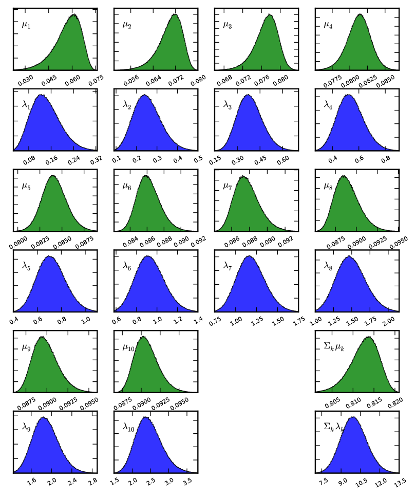
Having specified an ensemble of matrices from which to extract the eigenvalue spectra, we are now ready to perform numerical simulations. To begin with, we report in Fig. 3 the marginal probability density function of the ordered eigenvalues $\{\lambda_{k}\}_{k=1}^{v}$ and their truncated counterparts $\{\mu_{k}\}_{k=1}^{v}$ for the Wishart ensemble ${\cal W}_{10}(20,20^{-1}\cdot\mathds{I}_{10})$ at $\rho=1$, as obtained numerically from a rather large sample of matrices ($\simeq 10^{6}$ units). It will be noted that i) the effect of the truncation is severe on the largest eigenvalues, as a consequence of the analytic bounds of Corollary 2.1 and Proposition 2.2; ii) while the skewness of the lowest truncated eigenvalues is negative, it becomes positive for the largest ones. This is due to a change of relative effectiveness of eq. (3.17) i) with respect to eq. (3.17) ii).

6.2 Choice of the simulation parameters

In order to explore the dependence of ${\bar{n}}_{\rm it}$ upon $\rho$, we need to choose one or more simulation points for the latter. Ideally, it is possible to identify three different regimes in our problem: $\rho\lesssim\lambda_{1}$ (strong truncation regime), $\lambda_{1}\lesssim\rho\lesssim\lambda_{v}$ (crossover) and $\rho\gtrsim\lambda_{v}$ (weak truncation regime). We cover all of them with the following set of points:

$$\rho\,\in\,\left\{{{\rm Mo}(\lambda_{1})},\ \ldots\ ,\,{{\rm Mo}(\lambda_{v})}\right\}\,\cup\,\left\{\frac{1}{2}{{\rm Mo}(\lambda_{1})},\,2\,{{\rm Mo}(\lambda_{v})}\right\}\,,$$ (6.3)

	$v=3$	$v=4$	$v=5$	$v=6$	$v=7$	$v=8$	$v=9$	$v=10$
${{\rm\widehat{Mo}}(\lambda_{1})}$	0.1568	0.1487	0.1435	0.1383	0.1344	0.1310	0.1269	0.1258
${{\rm\widehat{Mo}}(\lambda_{2})}$	0.6724	0.4921	0.4017	0.3424	0.3039	0.2745	0.2554	0.2399
${{\rm\widehat{Mo}}(\lambda_{3})}$	1.6671	1.0112	0.7528	0.6071	0.5138	0.4543	0.4048	0.3693
${{\rm\widehat{Mo}}(\lambda_{4})}$	–	1.8507	1.2401	0.9621	0.7854	0.6684	0.5858	0.5288
${{\rm\widehat{Mo}}(\lambda_{5})}$	–	–	2.0150	1.4434	1.1269	0.9263	0.7956	0.7032
${{\rm\widehat{Mo}}(\lambda_{6})}$	–	–	–	2.1356	1.5789	1.2559	1.0527	0.9111
${{\rm\widehat{Mo}}(\lambda_{7})}$	–	–	–	–	2.2190	1.6764	1.3673	1.1603
${{\rm\widehat{Mo}}(\lambda_{8})}$	–	–	–	–	–	2.2763	1.7687	1.4624
${{\rm\widehat{Mo}}(\lambda_{9})}$	–	–	–	–	–	–	2.3210	1.8473
${{\rm\widehat{Mo}}(\lambda_{10})}$	–	–	–	–	–	–	–	2.3775

Table 1: Numerical estimates of the mode of the ordered eigenvalues $\{\lambda_{1},\dots,\lambda_{v}\}$ of $\Sigma\sim{\cal W}_{v}\left(2v,(2v)^{-1}\cdot\mathds{I}_{v}\right)$ with $v=3,\dots,10$. The estimates have been obtained from Grenander’s mode estimator [19].

where ${{\rm Mo}(\cdot)}$ stands for the mode. In principle, it is possible to determine ${{\rm Mo}(\lambda_{k})}$ with high accuracy by using analytic representations of the marginal probability densities of the ordered eigenvalues [20]. In practice, the latter become computationally demanding at increasingly large values of $v$: for instance, the determination of the probability density of $\lambda_{2}$ requires $(v!)^{2}$ sums, which is unfeasible even at $v\sim 10$. Moreover, to our aims it is sufficient to choose approximate values, provided these lie not far from the exact ones. Accordingly, we have determined the eigenvalue modes numerically from samples of $N\simeq 10^{6}$ Wishart matrices. Our estimates are reported in Table 1 for $v=3,\ldots,10$. They have been obtained from Grenander’s estimator [19],

$${{\rm Mo}(\lambda_{k})}_{rs}=\frac{1}{2}\frac{\sum_{i=1}^{N-r}\left(\lambda_{k}^{(i)}+\lambda_{k}^{(i+r)}\right)\left(\lambda_{k}^{(i)}-\lambda_{k}^{(i+r)}\right)^{-s}}{\sum_{i=1}^{N-r}\left(\lambda_{k}^{(i)}-\lambda_{k}^{(i+r)}\right)^{-s}}\,,$$ (6.4)

with properly chosen parameters $r$, $s$.

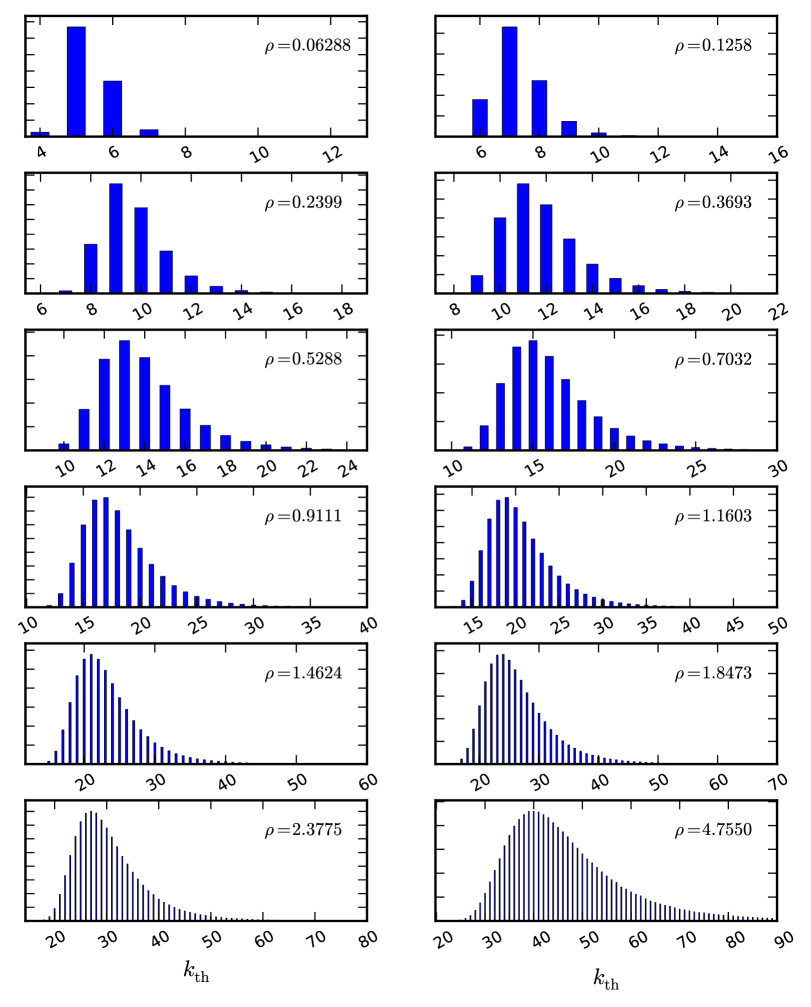
We are now in the position to investigate numerically how many terms in Ruben’s expansions must be considered as $\varepsilon$ is set to $\varepsilon_{\rm dp}=1.0\times 10^{-14}$, for our choice of the eigenvalue ensemble $\lambda\sim{\cal W}_{v}\left(2v,(2v)^{-1}\cdot\mathds{I}_{v}\right)$ and with $\rho$ set as in Table 1. As an example, we report in Fig. 4 the discrete distributions of ${k_{\rm th}}$ for the basic Gaussian integral $\alpha$ at $v=10$, the largest dimension we have simulated. As expected, we observe an increase of ${k_{\rm th}}$ with $\rho$. Nevertheless, we see that the number of Ruben’s components to be taken into account for a double precision result keeps altogether modest even in the weak truncation regime, which proves the practical usefulness of the chi–square expansions.

6.3 Fixed point iteration at work

The GJ iteration is too slow to be of practical interest. For instance, at $v=10$, $\rho\simeq{{\rm Mo}(\lambda_{1})}$ and ${\epsilon}_{\scriptscriptstyle\rm T}=1.0\times 10^{-7}$ (corresponding to a reconstruction of $\lambda$ with single floating–point precision) it is rather easy to extract realizations of $\mu$ which require $n_{\rm it}\simeq 15,000$ to converge. An improvement of the GJ scheme is achieved via over–relaxation (GJOR), i.e.

$$\left\{\begin{array}[]{l}\lambda_{{\scriptscriptstyle\rm GJOR},k}^{(0)}\,=\,\mu_{k}\,,\\[8.61108pt] \lambda_{{\scriptscriptstyle\rm GJOR},k}^{(n+1)}\,=\,\lambda_{{\scriptscriptstyle\rm GJOR},k}^{(n)}+\omega\left[T_{k}(\lambda_{{\scriptscriptstyle\rm GJOR}}^{(n)})-\lambda_{{\scriptscriptstyle\rm GJOR},k}^{(n)}\right]\,,\qquad k=1,\ldots,v\end{array}\right.\,.$$ (6.5)

Fig. 3: Monte Carlo simulation of the probability density function of the ordered eigenvalues $\lambda_{k}$ (even rows) and their truncated counterparts $\mu_{k}$ at $\rho=1$ (odd rows) for the Wishart ensemble ${\cal W}_{10}(20,20^{-1}\cdot\mathds{I}_{10})$. The last two plots (bottom right) display the distribution of the sum of eigenvalues.

Fig. 4: Monte Carlo simulation of the probability mass function of the parameter ${k_{\rm th}}$ for the Gaussian probability content $\alpha$. The histograms refer to the eigenvalue ensemble $\lambda$ of $\Sigma\sim{\cal W}_{10}(20,20^{-1}\cdot\mathds{I}_{10})$, with $\rho$ chosen as in Table 1 and $\varepsilon=1.0\times 10^{-14}$.

Evidently, at $\omega=1$ the GJOR scheme coincides with the standard GJ one. The optimal value $\omega_{\rm opt}$ of the relaxation factor $\omega$ is not obvious even in the linear Jacobi scheme, where $\omega_{\rm opt}$ depends upon the properties of the coefficient matrix of the system. For instance, if the latter is symmetric positive definite, it is demonstrated that the best choice is provided by $\omega_{\rm opt}\equiv~{}2(1+\sqrt{1-\sigma^{2}})^{-1}$, being $\sigma$ the spectral radius of the Jacobi iteration matrix [21]. In our numerical tests with the GJOR scheme, we found empirically that the optimal value of $\omega$ at $\rho\lesssim\lambda_{v}$ is close to the linear prediction, provided $\sigma$ is replaced by $||J||_{\infty}$, being $J$ defined as in sect. 3 (note that $||J||_{\infty}<1$). By contrast, the iteration diverges after few steps with increasing probability as $\rho/\lambda_{v}\to\infty$ if $\omega$ is kept fixed at $\omega=\omega_{\rm opt}$; in order to restore the convergence, $\omega$ must be lowered towards $\omega=1$ as such limit is taken.

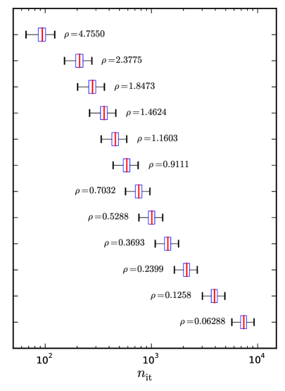
To give an idea of the convergence rate of the GJOR scheme, we show in Fig. 5 (left) a joint box–plot of the distributions of $n_{\rm it}$ at $v=10$ and ${\epsilon}_{\scriptscriptstyle\rm T}=1.0\times 10^{-7}$. From the plot we observe that the distribution of $n_{\rm it}$ shifts rightwards as $\rho$ decreases: clearly, the reconstruction is faster if $\rho$ is in the weak truncation regime (where $\mu$ is closer to $\lambda$), whereas it takes more iterations in the strong truncation regime. The dependence of ${\bar{n}}_{\rm it}$ upon $\rho$, systematically displayed in Fig. 6, is compatible with a scaling law

$$\log{\bar{n}}_{\rm it}(\rho,v,{\epsilon}_{\scriptscriptstyle\rm T})=a(v,{\epsilon}_{\scriptscriptstyle\rm T})-b(v,{\epsilon}_{\scriptscriptstyle\rm T})\log\rho\,,$$ (6.6)

$v$ ide$\hat{a}$ (jk.err.)ide ide$\hat{b}$ (jk.err.)ide 3 4.93(3) 0.940(1) 4 5.25(2) 0.940(1) 5 5.44(2) 0.948(1) 6 5.65(1) 0.953(1) 7 5.85(1) 0.948(1) 8 6.02(1) 0.951(1) 9 6.18(1) 0.946(1) 10 6.31(1) 0.948(1)

Fig. 5: (left) Box–plot of $n_{\rm it}$ in the GJOR scheme at $v=10$, with ${\epsilon}_{\scriptscriptstyle\rm T}=1.0\times 10^{-7}$ and $\rho$ chosen as in Table 1. The distributions have been reconstructed from a sample of $N\simeq 10^{3}$ eigenvalue spectra extracted from ${\cal W}_{10}(20,20^{-1}\cdot\mathds{I}_{10})$. The whiskers extend to the most extreme data point within $(3/2)(75\%-25\%)$ data range. (right) Numerical estimates of the scaling parameters $a$ and $b$ of the GJOR scheme, as obtained from jackknife fits to eq. (6.6) of data points with $\rho\lesssim 1$ and ${\epsilon}_{\scriptscriptstyle\rm T}=1.0\times 10^{-7}$. We quote in parentheses the jackknife error.

Fig. 6: Log–log plots of ${\bar{n}}_{\rm it}$ vs. $\rho$ in the GJOR scheme at ${\epsilon}_{\scriptscriptstyle\rm T}=1.0\times 10^{-7}$. The parameter $\rho$ has been chosen as in Table 1. The (red) dashed line in each plot represents our best jackknife linear fit to eq. (6.6) of data points with $\rho\lesssim 1$.

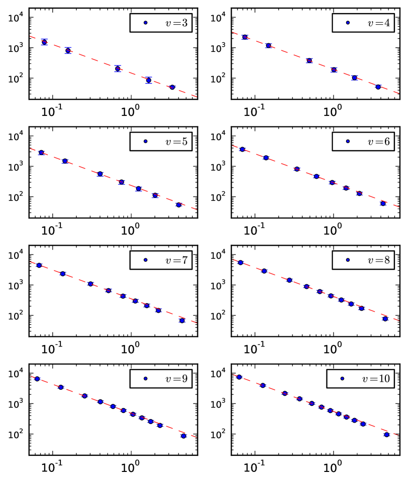
apart from small corrections occurring at large $\rho$. Eq. (6.6) tells us that ${\bar{n}}_{\rm it}$ increases polynomially in $1/\rho$ at fixed $v$. In order to estimate the parameters $a$ and $b$ in the strong truncation regime (where the algorithm becomes challenging), we performed jackknife fits to eq. (6.6) of data points with $\rho\lesssim 1$. Results are collected in Fig. 5 (right), showing that $b$ is roughly constant, while $a$ increases almost linearly in $v$. Thus, while the cost of the eigenvalue reconstruction is only polynomial in $1/\rho$ at fixed $v$, it is exponential in $v$ at fixed $\rho$. The scaling law of the GJOR scheme is therefore better represented by ${\bar{n}}_{\rm it}=C{\rm e}^{\kappa v}/\rho^{b}$, with $C$ being a normalization constant independent of $\rho$ and $v$, and $\kappa$ representing approximately the slope of $a$ as a function of $v$. Although the GJOR scheme improves the GJ one, the iteration reveals to be still inefficient in a parameter subspace, which is critical for the applications.

6.4 Boosting the GJOR scheme

A further improvement can be obtained by letting $\omega$ depend on the eigenvalue index in the GJOR scheme. Let us discuss how to work out such an adjustment. On commenting Fig. 3, we have already noticed that the largest eigenvalues are affected by the truncation to a larger extent than the smallest ones. Therefore, they must perform a longer run through the fixed point iteration, in order to converge to the untruncated values. This is a possible qualitative explanation for the slowing down of the algorithm as $\rho\to 0$. In view of it, we expect to observe some acceleration of the convergence rate, if $\omega$ is replaced, for instance, by

$$\omega\,\rightarrow\,\omega_{k}\,\equiv\,(1+\beta\cdot k)\,\omega_{\rm opt}\,,\qquad\beta\geq 0\,,\qquad k=1,\ldots,v\,.$$ (6.7)

The choice $\beta=0$ corresponds obviously to the standard GJOR scheme. Any other choice yields $\omega_{k}>\omega_{\rm opt}$. Therefore, the new scheme is also expected to display a higher rate of failures than the GJOR one at $\rho\gg\lambda_{v}$, for the reason explained in sect. 5.3. The component–wise over–relaxation proposed in eq. (6.7) is only meant to enhance the convergence speed in the strong truncation regime and in the crossover, where the improvement is actually needed.

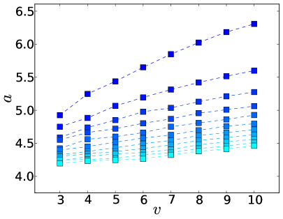
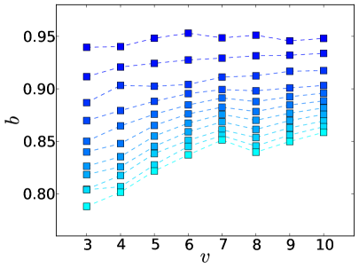
In order to confirm this picture, we have explored systematically the effect of $\beta$ on ${\bar{n}}_{\rm it}$ by simulating the reconstruction process at $v=3,\ldots,10$, with $\beta$ varying from 0 to 2 in steps of $1/5$. First of all, we have observed that the rate of failures at large $\rho$ is fairly reduced if the first $30\div 50$ iterations are run with $\omega_{k}=\omega_{\rm opt}$, and only afterwards $\beta$ is switched on. Having minimized the failures, we have checked that for each value of $\beta$, the scaling law assumed in eq. (6.6) is effectively fulfilled. Then, we have computed jackknife estimates of the scaling parameters $a$ and $b$. These are plotted in Fig. 7 as functions of $v$. Each trajectory (represented by a dashed curve) corresponds to a given value of $\beta$. Those with darker markers refer to smaller values of $\beta$ and the other way round. From the plots we notice that

• all the trajectories with $\beta>0$ lie below the one with $\beta=0$;
  

• the trajectories of $a$ display a clear increasing trend with $v$, yet their slope lessens as $\beta$ increases. By contrast, the trajectories of $b$ develop a mild increasing trend with $v$ as $\beta$ increases, though this is not strictly monotonic;
  

• the trajectories of both $a$ and $b$ seem to converge to a limit trajectory as $\beta$ increases; we observe a saturation phenomenon, which thwarts the benefit of increasing $\beta$ beyond a certain threshold close to $\beta_{\rm max}\simeq 2$.

We add that pushing $\beta$ beyond $\beta_{\rm max}$ is counterproductive, as the rate of failures becomes increasingly relevant in the crossover and eventually also in the strong truncation regime. By contrast, if $\beta\lesssim\beta_{\rm max}$ the rate of failures keeps very low for essentially all simulated values of $\rho$.

Fig. 7: Scaling parameters $a$ and $b$ of the modified GJOR scheme as functions of $v$ at ${\epsilon}_{\scriptscriptstyle\rm T}=1.0\times 10^{-7}$, with $\beta$ varying in the range $0\div 2$ in steps of $1/5$. Each trajectory (represented by a dashed curve) refers to a different value of $\beta$. Those with darker markers correspond to smaller values of $\beta$ and the other way round.

Fig. 8: The parameter $\kappa$ as a function of $\beta$. Estimates of $\kappa$ are obtained from least–squares fits of data to a linear model $a=a_{0}+\kappa\cdot v$.

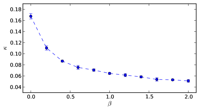
Our numerical results signal a strong reduction of the slowing down of the convergence rate. Indeed, i) means qualitatively that $C$ and $b$ are reduced as $\beta$ increases. ii) means that $\kappa$ is reduced as $\beta$ increases (this is the most important effect, as $\kappa$ is mainly responsible for the exponential slowing down with $v$). The appearance of a slope in the trajectories of $b$ as $\beta$ increases indicates that a mild exponential slowing down is also developed at denominator of the scaling law ${\bar{n}}_{\rm it}=C{\rm e}^{\kappa v}/\rho^{b}$, but the value of $b$ is anyway smaller than at $\beta=0$. Finally, iii) means that choosing $\beta>\beta_{\rm max}$ has a minor impact on the performance of the algorithm. In Fig. 8, we report a plot of the parameter $\kappa$ (obtained from least–squares fits of data to a linear model $a=a_{0}+\kappa\cdot v$) as a function of $\beta$. We see that $\kappa(\beta=0)/\kappa(\beta=2)\simeq 4$. This quantifies the maximum exponential speedup of the convergence rate, which can be achieved by our proposal. When $\beta$ is close to $\beta_{\rm max}$, ${\bar{n}}_{\rm it}$ amounts to few hundreds at $v=10$ and $\rho\simeq\lambda_{1}/2$.

7 On the ill–posedness of the reconstruction in sample space

So far we have discussed the covariance reconstruction under the assumption that $\mu=\tau_{\rho}\cdot\lambda$ represents the exact truncated counterpart of some $\lambda\in{\mathbb{R}}^{v}$ and we have looked at the algorithmic properties of the iteration schemes which operatively define $\tau^{-1}_{\rho}$. Such analysis is essential in order to characterize $\tau^{-1}_{\rho}$ mathematically, yet it is not sufficient in real situations, specifically when $\mu$ is perturbed by statistical noise.

In this section, we examine the difficulties arising when performing the covariance reconstruction in sample space. We first recall that according to Hadamard [22], a mathematical problem is well–posed provided the following conditions are fulfilled:

• there exists always a solution to the problem;

• the solution is unique;

• the solution depends smoothly on the input data.

Inverse problems are often characterized by violation of one or more of them, see for instance ref. [9]. In such cases, the standard practice consists in regularizing the inverse operator, i.e. in replacing it by a stable approximation. With regard to our problem, the reader will recognize that $H_{1}$ is violated (and the problem becomes ill–posed) as soon as the space of the input data is allowed to be a superset of ${\cal D}(\tau_{\rho}^{-1})$: once clarified how $\mu$ is concretely estimated in the applications (sects. 7.1 and 7.2), we propose a perturbative regularization of $\tau_{\rho}^{-1}$, which improves effectively the fulfillment of $H_{1}$ (sect. 7.3). By contrast, Proposition 4.3 guarantees that whenever a solution exists, it is also unique, thus $H_{2}$ is never of concern. Finally, the fulfillment of $H_{3}$ depends on how the statistical noise on $\mu$ is non–linearly inflated by the action of $\tau_{\rho}^{-1}$. For the sake of conciseness, in the present paper we just sketch the main ideas underlying the perturbative regularization of $\tau_{\rho}^{-1}$, whereas a technical implementation of it and a discussion of $H_{3}$ are deferred to a separate paper [23].

7.1 Definition of the sample truncated covariance matrix

The examples of sect. 2 assume that i) spherical truncations are operated on a representative sample ${\cal P}_{N}=\{x^{(k)}\}_{k=1}^{N}$ of $X\sim{\cal N}_{v}(0,\Sigma)$ with finite size $N$, ii) $\rho$ is known exactly and iii) the input budget for the covariance reconstruction is given by the subset

$${\cal Q}_{M}=\{x\in{\cal P}_{N}:\ ||x||^{2}<\rho\}\,,\qquad\text{with}\qquad|{\cal Q}_{M}|=M\leq N\,.$$ (7.1)

As usual in the analysis of stochastic variables in sample space, we assume that the observations $x^{(k)}$ are realizations of i.i.d. stochastic variables $X^{(k)}\sim{\cal N}_{v}(0,\Sigma)$, $k=1,\ldots,N$. Thus, $M$ is itself a stochastic variable in sample space, where it reads

$$M=\sum_{k=1}^{N}{\mathbb{I}}_{{\cal B}_{v}(\rho)}(X^{(k)})\equiv\sum_{k=1}^{N}{\mathbb{I}}_{k}\,,$$ (7.2)

with ${\mathbb{I}}_{{\cal B}_{v}(\rho)}(\cdot)$ denoting the characteristic function of ${\cal B}_{v}(\rho)$ and ${\mathbb{I}}_{k}\equiv{\mathbb{I}}_{{\cal B}_{v}(\rho)}(X^{(k)})$ being just a shortcut for its extended counterpart. It is easily recognized that $M\sim B(N,\alpha)$ is a binomial variate. If we indeed denote by $\mathfrak{E}$ the sample expectation operator (i.e. the integral with respect to the product measure of the joint variables $\{X^{(k)}\}_{k=1}^{N}$), then a standard calculation yields

$$\mathfrak{E}[M]={\mathfrak{E}}\left[\sum_{k=1}^{N}{\mathbb{I}}_{k}\right]=\sum_{k=1}^{N}{\mathfrak{E}}\left[{\mathbb{I}}_{k}\right]=\sum_{k=1}^{N}\alpha=\alpha N\,,$$ (7.3)

and

$${\mathfrak{var}}[M]={\mathfrak{E}}[M^{2}]-{\mathfrak{E}}[M]^{2}=\sum_{k=1}^{N}{\mathfrak{E}}\left[{\mathbb{I}}_{k}^{2}\right]+\sum_{k,s:\ k\neq s}^{1\ldots N}{\mathfrak{E}}\left[{\mathbb{I}}_{k}{\mathbb{I}}_{s}\right]-\alpha^{2}N^{2}$$

$$=\sum_{k=1}^{N}{\mathfrak{E}}\left[{\mathbb{I}}_{k}\right]+\sum_{k,s:\ k\neq s}^{1\ldots N}{\mathfrak{E}}\left[{\mathbb{I}}_{k}\right]{\mathfrak{E}}\left[{\mathbb{I}}_{s}\right]-\alpha^{2}N^{2}=\alpha N+\alpha^{2}N(N-1)-\alpha^{2}N^{2}=\alpha(1-\alpha)N\,.$$ (7.4)

Hence, we see that the relative dispersion of $M$ is $\text{O}(N^{-1/2})$. Now, the simplest way to measure $\Sigma$ and ${\mathfrak{S}}_{\cal B}$ respectively from the sets ${\cal P}_{N}$ and ${\cal Q}_{M}$ is via the classical estimators

$$\hat{\Sigma}_{ij} =\frac{1}{N-1}\sum_{x\in{\cal P}_{N}}(x-\bar{x})_{i}\,(x-\bar{x})_{j}\,, \bar{x}_{i}=\frac{1}{N}\sum_{x\in{\cal P}_{N}}x_{i}\,,$$ (7.5)

$$(\hat{\mathfrak{S}}_{\cal B})_{ij} =\frac{1}{M-1}\sum_{x\in{\cal Q}_{M}}(x-\tilde{x})_{i}\,(x-\tilde{x})_{j}\,, \tilde{x}_{i}=\frac{1}{M}\sum_{x\in{\cal Q}_{M}}x_{i}\,.$$ (7.6)

We define the sample estimates $\hat{\lambda}$ and $\hat{\mu}$ respectively of $\lambda$ and $\mu$ as the eigenvalue spectra of $\hat{\Sigma}$ and $\hat{\mathfrak{S}}_{\cal B}$. By symmetry arguments we see that $\tilde{x}_{i}$ is unbiased. Indeed, it holds

$$\mathfrak{E}[\tilde{x}_{i}]=\sum_{k=1}^{N}\mathfrak{E}\left[X_{i}^{(k)}\dfrac{{\mathbb{I}}_{k}}{\sum_{s=1}^{N}{\mathbb{I}}_{s}}\right]\,.$$ (7.7)

The r.h.s. of eq. (7.7) makes only sense if we conventionally define the integrand to be zero in the integration subdomain $\{X^{(k)}\notin{\cal B}_{v}(\rho),\ \forall k\}$, or equivalently if we interpret $\mathfrak{E}[\tilde{x}_{i}]$ as the conditional one $\mathfrak{E}[\tilde{x}_{i}\,|\,M>0]$ (the event $M>0$ occurs a.s. only as $N\to\infty$). Since the sample measure is even under $X^{(k)}\to-X^{(k)}$ while the integrand is odd, we immediately conclude that $\mathfrak{bias}[\tilde{x}_{i}]=0$.

7.2 Bias of the sample truncated covariance matrix

The situation gets somewhat less trivial with $\hat{\mathfrak{S}}_{\cal B}$: the normalization factor $(M-1)^{-1}$, which has been chosen in analogy with eq. (7.5), is not sufficient to remove completely the bias of $\hat{\mathfrak{S}}_{\cal B}$ at finite $N$, though we aim at showing here that the residual bias is exponentially small and asymptotically vanishing. In order to see this, we observe

$$\mathfrak{E}\left[(\hat{\mathfrak{S}}_{\cal B})_{ij}\right]=\sum_{k=1}^{N}\mathfrak{E}\left[\left(X^{(k)}_{i}-\tilde{X}_{i}\right)\left(X^{(k)}_{j}-\tilde{X}_{j}\right)\dfrac{{\mathbb{I}}_{k}}{\sum_{s=1}^{N}{\mathbb{I}}_{s}-1}\right]$$

$$=\sum_{\ell,r=1}^{v}R_{i\ell}R_{jr}\sum_{k=1}^{N}\mathfrak{E}_{\text{diag}}\left[\left(X^{(k)}_{\ell}-\tilde{X}_{\ell}\right)\left(X^{(k)}_{r}-\tilde{X}_{r}\right)\dfrac{{\mathbb{I}}_{k}}{\sum_{s=1}^{N}{\mathbb{I}}_{s}-1}\right]\,,$$ (7.8)

with $\mathfrak{E}_{\text{diag}}$ denoting the sample expectation corresponding to a multinormal measure with diagonal covariance matrix $\Lambda={\rm diag}(\lambda)={R}^{\scriptscriptstyle{\rm T}}\Sigma R$, conditioned to $M>1$. Having diagonalized the product measure, we observe that the integrand on the r.h.s. is odd for $\ell\neq r$ and even for $\ell=r$ under the joint change of variables $X^{(k)}_{\ell}\to-X^{(k)}_{\ell}$ for $k=1,\ldots,N$, similarly to what we did in sect. 2. As a consequence, it holds

$$\mathfrak{E}\left[(\hat{\mathfrak{S}}_{\cal B})_{ij}\right]=\sum_{\ell=1}^{v}R_{i\ell}R_{j\ell}\left\{\sum_{k=1}^{N}\mathfrak{E}_{\text{diag}}\left[\left(X^{(k)}_{\ell}-\tilde{X}_{\ell}\right)^{2}\dfrac{{\mathbb{I}}_{k}}{\sum_{s=1}^{N}{\mathbb{I}}_{s}-1}\right]\right\}\,,$$ (7.9)

whence we infer that the matrix $\mathfrak{E}[\hat{\mathfrak{S}}_{\cal B}]$ is diagonalized by the same matrix $R$ as $\Sigma$. From eq. (7.9) we also conclude that

$$\mathfrak{bias}[{\hat{\mathfrak{S}}_{\cal B}}]=R\,{\rm diag}(w)\,{R}^{\scriptscriptstyle{\rm T}},\qquad w_{i}\equiv\sum_{k=1}^{N}\mathfrak{E}_{\text{diag}}\left[\left(X^{(k)}_{i}-\tilde{X}_{i}\right)^{2}\dfrac{{\mathbb{I}}_{k}}{\sum_{s=1}^{N}{\mathbb{I}}_{s}-1}\right]-\mu_{i}\,,$$ (7.10)

$i=1,\ldots,v$. It should be observed that in general $w_{i}\neq\mathfrak{bias}[\hat{\mu}_{i}]$ since the computation of $\hat{\mu}_{i}$ requires the diagonalization of ${\hat{\mathfrak{S}}_{\cal B}}$, which is in general performed by a diagonalizing matrix $\hat{R}\neq R$. Nevertheless, if $w$ vanishes then $\mathfrak{bias}[{\hat{\mathfrak{S}}_{\cal B}}]$ vanishes too. Now, we observe that $w_{i}$ splits into three contributions,

$$w_{i1} =\phantom{-2}\sum_{k=1}^{N}\mathfrak{E}_{\text{diag}}\left[\left(X^{(k)}_{i}\right)^{2}\dfrac{{\mathbb{I}}_{k}}{\sum_{s=1}^{N}{\mathbb{I}}_{s}-1}\right]-\mu_{i}\,,$$ (7.11)

$$w_{i2} =-2\sum_{k=1}^{N}\mathfrak{E}_{\text{diag}}\left[X^{(k)}_{i}\tilde{X}_{i}\dfrac{{\mathbb{I}}_{k}}{\sum_{s=1}^{N}{\mathbb{I}}_{s}-1}\right]\,,$$ (7.12)

$$w_{i3} =\phantom{-2}\sum_{k=1}^{N}\mathfrak{E}_{\text{diag}}\left[\left(\tilde{X}_{i}\right)^{2}\dfrac{{\mathbb{I}}_{k}}{\sum_{s=1}^{N}{\mathbb{I}}_{s}-1}\right]\,,$$ (7.13)

which can be exactly calculated and expressed in terms of $\mu_{i}$, $\alpha$ and $N$. For instance,

$$w_{i1} =N\mathfrak{E}_{\text{diag}}\left[\frac{1}{M-1}(X_{i}^{(1)})^{2}{\mathbb{I}}_{1}\,\biggr{|}\,M>1\right]-\mu_{i}$$

$$=N\sum_{m=2}^{N}\frac{1}{m-1}\mathfrak{E}_{\text{diag}}\left[(X_{i}^{(1)})^{2}{\mathbb{I}}_{1}\,|\,M=m\right]-\mu_{i}$$

$$=N\sum_{m=2}^{N}\frac{1}{m-1}\alpha\mu_{i}{N-1\choose m-1}\alpha^{m-1}(1-\alpha)^{N-m}-\mu_{i}$$

$$=\mu_{i}\sum_{m=2}^{N}\frac{m}{m-1}{N\choose m}\alpha^{m}(1-\alpha)^{N-m}-\mu_{i}\,.$$ (7.14)

Analogously, we have

$$w_{i2}=-2\mu_{i}\sum_{m=2}^{N}\frac{1}{m-1}{N\choose m}\alpha^{m}(1-\alpha)^{N-m}\,,$$ (7.15)

$$w_{i3}=\phantom{-2}\mu_{i}\sum_{m=2}^{N}\frac{1}{m-1}{N\choose m}\alpha^{m}(1-\alpha)^{N-m}\,.$$ (7.16)

Hence, it follows

$$w_{i}=-\mu_{i}[1+\alpha(N-1)](1-\alpha)^{N-1}\,.$$ (7.17)

Since $\alpha>0$, we see that $\lim_{N\to\infty}w_{i}=0$. Thus, we conclude that ${\hat{\mathfrak{S}}_{\cal B}}$ is asymptotically unbiased.

Fig. 9: Left: numerical reconstruction of the failure probability of the iterative procedure as $v=4$ and $\Sigma={\rm diag}(0.1,0.3,0.8,2.2)$, for several values of $\rho$ and for $N=200,250,\ldots,1000$. Right: failure probability of the perturbative regularization with same parameters.

A discussion of the variance of the sample truncated covariance matrix is beyond the scope of the present paper. We just observe that, apart from the above calculation, studying the sample properties of the truncated spectrum is made hard by the fact that eigenvalues and eigenvectors of a diagonalizable matrix are intimately related from their very definition, thus such study would require a careful consideration of the distribution of the sample diagonalizing matrix $\hat{R}\neq R$ of ${\hat{\mathfrak{S}}}_{B}$.

7.3 Perturbative regularization of $\tau_{\rho}^{-1}$

When $\mu$ is critically close to the internal boundary of ${\cal D}(\tau_{\rho}^{-1})$, a sample estimate $\hat{\mu}$ may fall outside of it due to statistical fluctuations. In that case the iterative procedure described in the previous sections diverges. On the quantitative side, the ill-posedness of the reconstruction problem is measured by the failure probability

$$p_{\text{fail}}(\rho,\Sigma,N)=\mathds{P}\left[\,\hat{\mu}\notin{\cal D}(\tau_{\rho}^{-1})\ \bigr{|}\ X^{(k)}\sim{\cal N}_{v}\left(0;\Sigma\right)\,,\ k=1,\ldots,N\,\right]\,,$$ (7.18)

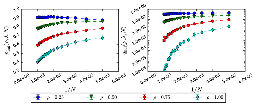
which is a highly non–trivial function of $\rho$, $\Sigma$ and $N$. An illustrative example of it is reported in Fig. 9 (left), which refers to a specific case with $v=4$ and $\Sigma={\rm diag}(0.1,0.3,0.8,2.2)$. The plot suggests that the iterative procedure becomes severely ill–posed in the regime of strong truncation.

In order to regularize the problem, we propose to go back to eq. (3.7) and consider it from a different perspective. Specifically, we move from the observation that a simplified framework occurs in the special circumstance when the eigenvalue spectra are fully degenerate, which is essentially equivalent to the set–up of ref. [1]. If $\mu_{1}=\ldots=\mu_{v}\equiv\tilde{\mu}$, by symmetry arguments it follows $\lambda_{1}=\ldots=\lambda_{v}\equiv\tilde{\lambda}$ and the other way round. Eq. (3.7) reduces in this limit to

$$\tilde{\mu}=\tilde{\lambda}\frac{F_{v+2}}{F_{v}}\left(\frac{\rho}{\tilde{\lambda}}\right)\equiv{\cal T}_{\rho}(\tilde{\lambda})\,,$$ (7.19)

It can be easily checked that the function ${\cal T}_{\rho}(\tilde{\lambda})$ is monotonic increasing in $\tilde{\lambda}$. In addition, we have

$$i\text{)}\quad\lim_{\tilde{\lambda}\to 0}{\cal T}_{\rho}(\tilde{\lambda})=0\,,\qquad\qquad ii\text{)}\lim_{\tilde{\lambda}\to\infty}{\cal T}_{\rho}(\tilde{\lambda})=\frac{\rho}{v+2}\,,$$ (7.20)

thus eq. (7.19) can be surely (numerically) inverted provided $0<\tilde{\mu}<\rho/(v+2)$. We can regard eq. (7.19) as an approximation to the original problem, eq. (3.7). When $\mu$ is not degenerate, we must define $\tilde{\mu}$ in terms of the components of $\mu$. One possibility is to average them, i.e. to choose

$$\tilde{\mu}=\frac{1}{v}\sum_{i=1}^{v}\mu_{i}\,.$$ (7.21)

Subject to this, we expect $\tilde{\lambda}$ to lie somewhere between $\lambda_{1}$ and $\lambda_{v}$. Eq. (7.19) can be thought of as the lowest order approximation of a perturbative expansion of eq. (3.7) around the point $\lambda_{\text{T}}=\{\tilde{\lambda},\ldots,\tilde{\lambda}\}$. If the condition number of $\Sigma$ is not extremely large, such an expansion is expected to quickly converge, so that a few perturbative corrections to $\lambda_{\text{T}}$ should be sufficient to guarantee a good level of approximation.

         a

Fig. 10: Left: set difference ${\cal D}({\cal T}_{\rho}^{-1})\setminus{\cal D}(\tau_{\rho}^{-1})$ in $v=2$ dimensions. Right: set difference ${\cal D}({\cal T}_{\rho}^{-1})\setminus{\cal D}(\tau_{\rho}^{-1})$ in $v=3$ dimensions.

As mentioned above, a technical implementation of the perturbative approach and a thorough discussion of its properties are deferred to a separate paper [23]. Here, we limit ourselves to observing that the definition domain of perturbation theory is ultimately set by its lowest order approximation, since corrections to eq. (7.19) are all algebraically built in terms of it, with no additional constraints. Following eq. (7.21), the domain of ${\cal T}_{\rho}^{-1}$ comes to be defined as

$${\cal D}({\cal T}_{\rho}^{-1})=\left\{\mu\in{\mathbb{R}}^{v}_{+}:\ \ \sum_{i=1}^{v}\mu_{i}\leq\frac{\rho v}{v+2}\right\}\,,$$ (7.22)

and it is clear that ${\cal D}(\tau_{\rho}^{-1})\subset{\cal D}({\cal T}_{\rho}^{-1})$ (it is sufficient to sum term by term all the inequalities contributing to eq. (3.24)). In Fig. 10, we show the set difference ${\cal D}({\cal T}_{\rho}^{-1})\setminus{\cal D}(\tau_{\rho}^{-1})$ in $v=2$ and $v=3$ dimensions. When $\mu\in{\cal D}(\tau_{\rho}^{-1})$ but its estimate $\hat{\mu}\notin{\cal D}(\tau_{\rho}^{-1})$, it may well occur $\hat{\mu}\in{\cal D}({\cal T}_{\rho}^{-1})$, i.e. the set difference acts as an absorbing shield of the statistical noise. Therefore, if we define the failure probability of the perturbative reconstruction as

$$q_{\text{fail}}(\rho,\Sigma,N)=\mathds{P}\left[\,\hat{\mu}\notin{\cal D}({\cal T}_{\rho}^{-1})\ \bigr{|}\ X^{(k)}\sim{\cal N}_{v}\left(0;\Sigma\right)\,,\ k=1,\ldots,N\,\right]\,,$$ (7.23)

we expect the inequality $q_{\text{fail}}(\rho,\Sigma,N)\ll p_{\text{fail}}(\rho,\Sigma,N)$ to generously hold. An example is given in Fig. 9 (right): we see that $q_{\text{fail}}$ becomes lower than $p_{\text{fail}}$ by orders of magnitude as soon as $\rho$ and $N$ are not exceedingly small. In this sense, the operator ${\cal T}_{\rho}^{-1}$ can be regarded as the lowest order approximation of a regularizing operator for $\tau_{\rho}^{-1}$.

8 Conclusions

In this paper we have studied how to reconstruct the covariance matrix $\Sigma$ of a normal multivariate $X\sim{\cal N}_{v}(0,\Sigma)$ from the matrix ${\mathfrak{S}}_{\cal B}$ of the spherically truncated second moments, describing the covariances among the components of $X$ when the probability density is cut off outside a centered Euclidean ball. We have shown that $\Sigma$ and ${\mathfrak{S}}_{{\cal B}}$ share the same eigenvectors. Therefore, the problem amounts to relating the eigenvalues of $\Sigma$ to those of ${\mathfrak{S}}_{{\cal B}}$. Such relation entails the inversion of a system of non–linear integral equations, which admits unfortunately no closed–form solution. Having found a necessary condition for the invertibility of the system, we have shown that the eigenvalue reconstruction can be achieved numerically via a converging fixed point iteration. In order to prove the convergence, we rely ultimately upon some probability inequalities, known in the literature as square correlation inequalities, which have been recently proved in [13].

In order to explore the convergence rate of the fixed point iteration, we have implemented some variations of the non–linear Gauss–Jacobi scheme. Specifically, we have found that over–relaxing the basic iteration enhances the convergence rate by a moderate factor. However, the over–relaxed algorithm still slows down exponentially in the number of eigenvalues and polynomially in the truncation radius of the Euclidean ball. We have shown that a significant reduction of the slowing down can be achieved in the regime of strong truncation by adapting the relaxation parameter to the eigenvalue it is naturally associated with, so as to boost the higher components of the spectrum.

We have also discussed how the iterative procedure works when the eigenvalue reconstruction is performed on sample estimates of the truncated covariance spectrum. Specifically, we have shown that the statistical fluctuations make the problem ill–posed. We have sketched a possible way–out based on perturbation theory, which is thoroughly discussed in a separate paper [23].

A concrete implementation of the proposed approach requires the computation of a set of multivariate Gaussian integrals over the Euclidean ball. For this, we have extended to the case of interest a technique, originally proposed by Ruben for representing the probability content of quadratic forms of normal variables as a series of chi–square distributions. In the paper, we have shown the practical feasibility of the series expansion for the integrals involved in our computations.

Appendix A Proof of Theorem 5.1

As already mentioned in sect. 4, the proof follows in the tracks of the original one of ref. [2]. We detail the relevant steps for $\alpha_{k}$, while for $\alpha_{jk}$ we only explain why it is necessary to distinguish between equal or different indices and the consequences for either case.

In order to prove eq. (5.7), we first express $\alpha_{k}$ in spherical coordinates, i.e. we perform the change of variable $x=ru$, being $r=||x||$ and $u\in\partial{\cal B}_{v}(1)$ (recall that ${\rm d}^{v}x=r^{v-1}{\rm d}r\,{\rm d}u$, with ${\rm d}u$ embodying the angular part of the spherical Jacobian and the differentials of $v-1$ angles); then we insert a factor of $1=\exp(r^{2}/2s)\exp(-r^{2}/2s)$ under the integral sign. Hence, $\alpha_{k}$ reads

$$\alpha_{k}(\rho;\lambda)=\frac{1}{(2\pi)^{v/2}|\Lambda|^{1/2}}\int_{0}^{\sqrt{\rho}}{\rm d}r\,r^{v-1}\frac{r^{2}}{\lambda_{k}}\exp\left(-\frac{r^{2}}{2s}\right)\int_{\partial{\cal B}_{v}(1)}{\rm d}u\ u_{k}^{2}\exp\left(-\frac{Q(u)r^{2}}{2}\right)\,.$$ (A.1)

The next step consists in expanding the inner exponential in Taylor series, viz.

$$\exp\left(-\frac{Q(u)r^{2}}{2}\right)\,=\,\sum_{m=0}^{\infty}\,\frac{1}{m!}\frac{r^{2m}}{2^{m}}(-Q)^{m}\,.$$ (A.2)

This series converges uniformly in $u$. We review the estimate just for the sake of completeness:

$$\left|\sum_{m=0}^{\infty}\,\frac{1}{m!}\frac{r^{2m}}{2^{m}}(-Q)^{m}\right|\leq\sum_{m=0}^{\infty}\frac{1}{m!}\frac{r^{2m}}{2^{m}}q_{0}^{m}=\exp\left(\frac{r^{2}q_{0}}{2}\right)\,,$$ (A.3)

being $q_{0}=\max_{i}|1/s-1/\lambda_{i}|$. It follows that we can integrate the series term by term. With the help of the uniform average operator introduced in eq. (5.3), $\alpha_{k}$ is recast to

$$\alpha_{k}(\rho;\lambda)=\sum_{m=0}^{\infty}\frac{1}{m!}\frac{1}{\lambda_{k}}\frac{1}{|\Lambda|^{1/2}}{\mathbb{M}}[(-Q)^{m}u_{k}^{2}]\frac{1}{2^{v/2+m-1}\Gamma(v/2)}\int_{0}^{\sqrt{\rho}}{\rm d}r\,r^{v+2m+1}\exp\left(-\frac{r^{2}}{2s}\right)\,.$$ (A.4)

The presence of an additional factor of $u_{k}^{2}$ in the angular average is harmless, since $|u_{k}^{2}|<1$. We finally notice that the radial integral can be expressed in terms of a cumulative chi–square distribution function on replacing $r\to\sqrt{rs}$, namely

$$\int_{0}^{\sqrt{\rho}}{\rm d}r\,r^{v+2m+1}\exp\left(-\frac{r^{2}}{2s}\right)\,=\,2^{v/2+m}s^{v/2+m+1}\Gamma\left(\frac{v}{2}+m+1\right)F_{v+2(m+1)}\left(\frac{\rho}{s}\right)\,.$$ (A.5)

Inserting eq. (A.5) into eq. (A.4) results in Ruben’s representation of $\alpha_{k}$. This completes the first part of the proof.

As a next step, we wish to demonstrate that the function $\psi_{k}$ of eq. (5.11) is the generating function of the coefficients $c_{k;m}$. To this aim, we first recall the identities

$$a^{-1/2} \,=\,(2\pi)^{-1/2}\int_{-\infty}^{\infty}{\rm d}x\,\phantom{x^{2}}\exp\left(-\frac{a}{2}x^{2}\right)\,,$$ (A.6)

$$a^{-3/2} \,=\,(2\pi)^{-1/2}\int_{-\infty}^{\infty}{\rm d}x\,x^{2}\exp\left(-\frac{a}{2}x^{2}\right)\,,$$ (A.7)

valid for $a>0$. On setting $a_{i}=[1-(1-s/\lambda_{i})z]$, we see that $\psi_{k}$ can be represented in the integral form

$$\psi_{k}(z) =\,\left(\frac{s}{\lambda_{k}}\right)^{3/2}(2\pi)^{-v/2}\int_{-\infty}^{\infty}{\rm d}x_{k}\,x_{k}^{2}\exp\left(-\frac{1}{2}\left[1-\left(1-\frac{s}{\lambda_{k}}\right)z\right]x_{k}^{2}\right)$$

$$\times\,\prod_{i\neq k}\left(\frac{s}{\lambda_{i}}\right)^{1/2}\int_{-\infty}^{\infty}{\rm d}x_{i}\,\exp\left(-\frac{1}{2}\left[1-\left(1-\frac{s}{\lambda_{k}}\right)z\right]x_{i}^{2}\right)$$

$$=\,\frac{s}{\lambda_{k}}\frac{s^{v/2}}{(2\pi)^{v/2}|\Lambda|^{1/2}}\int_{{\mathbb{R}}^{v}}{\rm d}^{v}x\,x_{k}^{2}\,\exp\left(-\frac{1}{2}zsQ(x)-\frac{{x}^{\scriptscriptstyle{\rm T}}\cdot x}{2}\right)\,,$$ (A.8)

provided $|z|<\min_{i}|1-s/\lambda_{i}|^{-1}$. As previously done, we introduce spherical coordinates $x=ru$, and expand $\exp\{-\frac{1}{2}zsQ(x)\}=\exp\{-\frac{1}{2}zsr^{2}Q(u)\}$ in Taylor series. By the same argument as above, the series converges uniformly in $u$ (the factor of $zs$ does not depend on $u$), thus allowing term by term integration. Accordingly, we have

$$\psi_{k}(z)=\frac{s}{\lambda_{k}}\frac{s^{v/2}}{(2\pi)^{v/2}|\Lambda|^{1/2}}\sum_{m=0}^{\infty}z^{m}\,\frac{s^{m}}{2^{m}m!}\int_{0}^{\infty}{\rm d}r\,r^{v+2(m+1)-1}{\rm e}^{-r^{2}/2}\int_{\partial{\cal B}_{v}(1)}{\rm d}u\,[-Q(u)]^{m}u_{k}^{2}\,.$$ (A.9)

We see that the r.h.s. of eq. (A.9) looks similar to eq. (A.4), the only relevant differences being the presence of the factor of $z^{m}$ under the sum sign and the upper limit of the radial integral. With some algebra, we arrive at

$$\psi_{k}(z)=\sum_{m=0}^{\infty}z^{m}\left\{\frac{2}{m!}\,\frac{s}{\lambda_{k}}\,\frac{s^{v/2+m}}{|\Lambda|^{1/2}}\,\frac{\Gamma(v/2+m+1)}{\Gamma(v/2)}\,{\mathbb{M}}[(-Q)^{m}u_{k}^{2}]\right\}\,.$$ (A.10)

The series coefficients are recognized to be precisely those of eq. (5.9).

In the last part of the proof, we derive the recursion fulfilled by the coefficients $c_{k;m}$. To this aim, the $m^{\rm th}$ derivative of $\psi_{k}$ has to be evaluated at $z=0$ and then identified with $m!\,c_{k;m}$. The key observation is that differentiating $\psi_{k}$ reproduces $\psi_{k}$ itself, that is to say

$$\psi^{\prime}_{k}(z)=\Psi_{k}(z)\psi_{k}(z)\,,$$ (A.11)

with

$$\Psi_{k}(z)=\frac{1}{2}\sum_{i=1}^{v}e_{k;i}\left(1-\frac{s}{\lambda_{i}}\right)\left[1-\left(1-\frac{s}{\lambda_{i}}\right)z\right]^{-1}\,,$$ (A.12)

and the auxiliary coefficient $e_{k;i}$ being defined as in eq. (5.20). Eq. (A.11) lies at the origin of the recursion. Indeed, from eq. (A.11) it follows that that $\psi_{k}^{\prime\prime}$ is a function of $\psi_{k}^{\prime}$ and $\psi_{k}$, viz. $\psi_{k}^{\prime\prime}=\Psi_{k}^{\prime}\psi_{k}+\Psi_{k}\psi_{k}^{\prime}$. Proceeding analogously yields the general formula

$$\psi_{k}^{(m)}(z)=\sum_{r=0}^{m-1}\binom{m-1}{r}\Psi_{k}^{(m-r-1)}(z)\,\psi_{k}^{(r)}(z)\,.$$ (A.13)

At $z=0$, this reads

$$m!\,c_{k;m}=\sum_{r=0}^{m-1}\frac{(m-1)!}{(m-r-1)!\,r!}\Psi_{k}^{(m-r-1)}(0)\ r!\,c_{k;r}\,.$$ (A.14)

The last step consists in proving that

$$\Psi_{k}^{(m)}(0)=\frac{1}{2}m!g_{k;m+1}\,,$$ (A.15)

with $g_{k;m}$ defined as in eq. (5.16). This can be done precisely as explained in ref. [2].

Having reiterated Ruben’s proof explicitly in a specific case, it is now easy to see how the theorem is extended to any other Gaussian integral. First of all, from eq. (A.1) we infer that each additional subscript in $\alpha_{k\ell m\ldots}$ enhances the power of the radial coordinate under the integral sign by 2 units. This entails a shift in the number of degrees of freedom of the chi–square distributions in Ruben’s expansion, amounting to twice the number of subscripts. For instance, since $\alpha_{jk}$ has two subscripts, its Ruben’s expansion starts by $F_{v+4}$, independently of whether $j=k$ or $j\neq k$. In second place, we observe that in order to correctly identify the generating functions of Ruben’s coefficients for a higher–order integral $\alpha_{k\ell m\ldots}$, we need to take into account the multiplicities of the indices $k$, $\ell$, $m$,…. As an example, consider the case of $\psi_{jk}$ ($j\neq k$) and $\psi_{kk}$. By going once more through the argument presented in eq. (A), we see that eqs. (A.6)–(A.7) are sufficient to show that eq. (5.1) is the generating function of $\alpha_{jk}$. By contrast, in order to repeat the proof for the case of $\psi_{kk}$, we need an additional integral identity, namely

$$a^{-5/2}\,=\,\frac{1}{3}\,(2\pi)^{-1/2}\int_{-\infty}^{+\infty}{\rm d}x\,x^{4}\exp\left(-\frac{a}{2}x^{2}\right)\,,$$ (A.16)

valid once more for $a>0$. Hence, we infer that $\psi_{kk}$ must depend upon $\lambda_{k}$ via a factor of $[1-(1-s/\lambda_{k})z]^{-5/2}$, whereas $\psi_{jk}$ ($j\neq k$) must depend on $\lambda_{j}$ and $\lambda_{k}$ via factors of resp. $[1-(1-s/\lambda_{j})z]^{-3/2}$ and $[1-(1-s/\lambda_{k})z]^{-3/2}$. The different exponents are ultimately responsible for the specific values taken by the auxiliary coefficients $e_{kk;i}$ and $e_{jk;i}$ of eq. (5.25).

To conclude, we observe that the estimates of the residuals ${\cal R}_{k;m}$ and ${\cal R}_{jk;m}$, presented in sect. 4 without an explicit proof, do not require any further technical insight than already provided by ref. [2] plus our considerations. We leave them to the reader, since they can be obtained once more in the tracks of the original derivation of ${\cal R}_{m}$.

References

- [1] G. M. Tallis. Elliptical and radial truncation in normal populations. The Annals of Mathematical Statistics, 34(3):940–944, 1963.
- [2] H. Ruben. Probability content of regions under spherical normal distributions, iv: The distribution of homogeneous and non-homogeneous quadratic functions of normal variables. The Annals of Mathematical Statistics, 33(2):542–570, 1962.
- [3] J. Aitchison. The statistical analysis of compositional data. Monographs on statistics and applied probability. Chapman and Hall, 1986.
- [4] V. Pawlowsky-Glahn and A. Buccianti. Compositional Data Analysis: Theory and Applications. Wiley, 2011.
- [5] J. J. Egozcue, V. Pawlowsky-Glahn, G. Mateu-Figueras, and C. Barceló-Vidal. Isometric logratio transformations for compositional data analysis. Mathematical Geology, 35:279–300, 2003.
- [6] J. Aitchison and S. Shen. Logistic Normal Distributions: Some Properties and Uses. Biometrika, 67(2):261–272, 1980.
- [7] V Pawlowsky-Glahn and J. J. Egozcue. Geometric approach to statistical analysis on the simplex. Stochastic Environmental Research and Risk Assessment, 15:384–398, 2001.
- [8] H.W. Engl, M. Hanke, and A. Neubauer. Regularization of Inverse Problems. Mathematics and Its Applications. Springer, 1996.
- [9] Laurent Cavalier. Inverse problems in statistics. In Pierre Alquier, Eric Gautier, and Gilles Stoltz, editors, Inverse Problems and High-Dimensional Estimation, Lecture Notes in Statistics, pages 3–96. Springer Berlin Heidelberg, 2011.
- [10] F. Palombi and S. Toti. A note on the variance of the square components of a normal multivariate within a Euclidean ball. Journal of Multivariate Analysis, 122:355–376, 2013.
- [11] M. Anttila, K. Ball, and I. Perissinaki. The central limit problem for convex bodies. Transactions of the American Mathematical Society, 355:4723–4735, 2003.
- [12] J. Onufry Wojtaszczyk. The square negative correlation property for generalized Orlicz balls. Geometric Aspects of Functional Analysis, Israel Seminar, pages 305–313, 2004–2005, 0803.0433.
- [13] R. Mukerjee and S. H. Ong. Variance and Covariance Inequalities for Truncated Joint Normal Distribution via Monotone Likelihood Ratio and Log-concavity. ArXiv e-prints, 2013, 1311.6018.
- [14] F. G. Friedlander and M. S. Joshi. Introduction to the theory of distributions. Cambridge University Press, 1998.
- [15] M. Abramowitz and I. A. Stegun. Handbook of Mathematical Functions with Formulas, Graphs, and Mathematical Tables. Dover Publications, New York, 1964.
- [16] K. L. Judd. Numerical Methods in Economics. The MIT Press, 1998.
- [17] T. W. Anderson. An Introduction to Multivariate Statistical Analysis, 2nd Edition. Wiley, 2 edition, 1984.
- [18] M. S. Bartlett. On the theory of statistical regression. Proc. Roy. Soc. Edinburgh, 53:260–283, 1933.
- [19] U. Grenander. Some direct estimates of the mode. The Annals of Mathematical Statistics, 36(1):131–138, 1965.
- [20] A. Zanella, M. Chiani, and M. Z. Win. On the marginal distribution of the eigenvalues of wishart matrices. Trans. Comm., 57:1050–1060, 2009.
- [21] D. M. Young. Iterative solution of large linear systems. Computer science and applied mathematics. Academic Press, 1971.
- [22] Jacques Hadamard. Sur les problèmes aux dérivés partielles et leur signification physique. Princeton University Bulletin, 13:49–52, 1902.
- [23] F. Palombi and S. Toti. A perturbative approach to the reconstruction of the eigenvalue spectrum of a normal covariance matrix from a spherically truncated counterpart. ArXiv e-prints, 2012, 1207.1256.
- [24] see http://www.cresco.enea.it/english for information.