Measure and Probability in Cosmology

Abstract

General relativity has a Hamiltonian formulation, which formally provides a canonical (Liouville) measure on the space of solutions. In ordinary statistical physics, the Liouville measure is used to compute probabilities of macrostates, and it would seem natural to use the similar measure arising in general relativity to compute probabilities in cosmology, such as the probability that the universe underwent an era of inflation. Indeed, a number of authors have used the restriction of this measure to the space of homogeneous and isotropic universes with scalar field matter (minisuperspace)—namely, the Gibbons-Hawking-Stewart measure—to make arguments about the likelihood of inflation. We argue here that there are at least four major difficulties with using the measure of general relativity to make probability arguments in cosmology: (1) Equilibration does not occur on cosmological length scales. (2) Even in the minisuperspace case, the measure of phase space is infinite and the computation of probabilities depends very strongly on how the infinity is regulated. (3) The inhomogeneous degrees of freedom must be taken into account (we illustrate how) even if one is interested only in universes that are very nearly homogeneous. The measure depends upon how the infinite number of degrees of freedom are truncated, and how one defines “nearly homogeneous.” (4) In a universe where the second law of thermodynamics holds, one cannot make use of our knowledge of the present state of the universe to “retrodict” the likelihood of past conditions.

I Introduction

Some of the most fundamental issues in cosmology concern the state of the universe at its earliest moments, for which we have very little direct observational evidence. In this situation, it is natural to attempt to make probabilistic arguments to assess the plausibility of various possible scenarios. For example, one could try to argue that it is “highly improbable” that the universe could have been in a homogeneous, isotropic, and very nearly spatially flat initial state, so that a mechanism like inflation occurring in the very early universe is necessary to explain the observed homogeneity, isotropy, and long age of the present universe. Similarly, one could try to make arguments as to whether the occurrence of inflation itself in the early universe was “probable.” Clearly, in order to make any probabilistic arguments, one needs a measure on the state space of the universe. General relativity has a Hamiltonian formulation, so—formally, at least—it gives rise to a canonical measure on phase space. When restricted to minisuperspace, this canonical measure—known as the Gibbons-Hawking-Stewart (GHS) measure—has been used to make probabilistic arguments in cosmology, such as whether inflation was probable Gibbons et al. (1987); Hawking and Page (1988); Gibbons and Turok (2008); Carroll and Tam (2010). The main purpose of this paper is to provide critical examination of the use of these types of probability arguments in cosmology.

As we shall discuss in detail in section II, the phase space of general relativity has many similarities to finite dimensional phase spaces of classical particle systems, most importantly the existence of a symplectic form which is conserved under time evolution Lee and Wald (1990). However, there are also significant differences. General relativity is a field theory, so its phase space is infinite dimensional. In the finite dimensional case, one can get the conserved canonical (Liouville) measure by taking the top exterior product $\wedge^{n}\omega$ of the conserved symplectic form $\omega$. But in the infinite dimensional case this does not make sense. Thus, to get a canonical measure for general relativity, we must truncate the degrees of freedom by imposing long and short wavelength cutoffs, so that we are effectively reduced to finitely many degrees of freedom. A long wavelength cutoff is naturally imposed by assuming that the cosmological models under consideration have compact Cauchy surfaces. A short wavelength cutoff is effectively imposed by quantum theory and/or the weak coupling of the degrees of freedom of interest to very high energy modes. With the imposition of these cutoffs, a canonical measure can be obtained from $\omega$ as in the finite degrees of freedom case.

However, an even more significant difference between general relativity and ordinary Hamiltonian systems of particles concerns the presence of constraints and the nature of these constraints. On account of the Hamiltonian and momentum constraints, not all points of phase space are allowed initial data for solutions. Thus, one must restrict consideration to the submanifold, $\mathcal{C}$, of points of phase space that satisfy the constraints. However, when pulled back to $\mathcal{C}$, the symplectic form becomes degenerate. The degeneracy directions of the pullback, $\overline{\omega}$, of the symplectic form, $\omega$, to $\mathcal{C}$ are precisely the infinitesimal gauge transformations, i.e., the changes in initial data corresponding to performing infinitesimal spacetime diffeomorphisms on the corresponding solutions. One can remove this degeneracy in a natural manner by passing to the gauge equivalence classes of initial data, i.e., by considering a new phase space whose points correspond to physically distinct spacetime solutions. One can then define a canonical measure on (a truncated version of) this space. However this gives rise to a major, additional conceptual issue: “Gauge” (= spacetime diffeomorphisms) includes “time evolution,” so once “gauge” has been eliminated from the phase space, there is no longer any notion of “time evolution.” But in the absence of nontrivial time evolution, one cannot make any arguments concerning dynamical behavior, such as equilibration, the second law of thermodynamics, etc. Note that this is a classical version of the “problem of time” that arises in canonical quantum gravity.

This issue can be dealt with by choosing a representative of each gauge orbit rather than passing to the space of gauge orbits. “Time evolution” then gets replaced by “change of description” when a different representative of each gauge orbit is chosen. The main difficulty with proceeding in this manner is that it does not appear possible to choose a unique gauge representative globally in phase space in a continuous manner, so this strategy cannot be implemented globally. Nevertheless, it is plausible that Cauchy surfaces with constant mean curvature $K=K_{*}$ are unique in certain classes of “nearly FLRW” models with compact Cauchy surfaces. For the purposes of this paper, we will assume that the condition $K=K_{*}$ picks out a unique Cauchy surface in the spacetimes under consideration here. In that case, “time evolution” is replaced by “change of description” of initial data when the choice of representative Cauchy surface is changed from from $K=K_{*}$ to $K=K^{\prime}_{*}$. Thus, $K$ effectively plays the role of “time” York (1971); Marsden and Tipler (1980), and one recovers a notion of dynamical evolution, although with a “time dependent” Hamiltonian.

The above considerations bring general relativity to a framework that is close to the framework of ordinary statistical physics. In ordinary statistical physics, the canonical measure has been successfully used to make probability arguments, and one might attempt to make similar arguments in cosmology. However, there are a number of serious difficulties in doing so. As we shall discuss in section III, one difficulty concerns the effective time dependence of the Hamiltonian and the insufficient time for equilibration to have occurred on scales comparable to the Hubble radius, thereby removing the usual justification for the use of the canonical measure. Another serious problem concerns the fact that even in minisuperspace models, the phase space of general relativity is non-compact, and the total measure of phase space is infinite. Thus, the “probability” of any subset of phase space is either $0$ (if its measure is finite), $1$ (if the measure of its complement is finite), or ambiguous (if both the set and its complement have infinite measure). In section IV, we shall discuss the calculation of the “probability of inflation” and—in agreement with a much earlier discussion by Hawking and Page Hawking and Page (1988)—explain why different authors have obtained widely different results using ostensibly the same (conserved!) GHS measure on minisuperspace. In section V, we consider inhomogeneous degrees of freedom. We briefly discuss some of the additional difficulties that arise when considering the inhomogeneous degrees of freedom in cosmology, such as placing a “short wavelength cutoff” in an expanding universe. Most of section V is devoted to deriving the modifications of the GHS measure that take the effects of inhomogeneous perturbations into account. Finally, in section VI we discuss the fact that in a universe with a thermodynamic arrow of time, one cannot “retrodict” the past by knowing the present state of the universe and determining which histories are most “probable” in the canonical measure; the second law of thermodynamics guarantees that the actual history of a system is extremely rare in the space of all possible histories that are consistent with present course-grained observations.

We conclude this introduction by mentioning an issue that we will not address in this paper. The fact that we are conscious observers undoubtedly places a bias on our observations: We are only able to directly observe portions of spacetime that can admit the presence of conscious observers. Therefore, in order to obtain the probability that a region of spacetime will be observed to have a certain property, we should multiply the a priori probability of the existence of such a region of spacetime by the probability that conscious observers exist in this region. Unfortunately, there are few things we know less about in science than the conditions needed for the existence of conscious observers (or, indeed, even what “conscious observers” are). In many discussions, it is implicitly or explicitly assumed that various conditions we observe to occur in our universe are necessary for conscious observers to exist. It therefore should not be surprising if the conclusion then drawn is that the universe should look similar to what we observe it to be, even if the a priori probability of what we observe (without taking into account the bias of our existence) is extremely small. Thus, although such anthropic arguments can be used to attempt to salvage a theory that predicts a very small a priori probability for what we observe, we do not feel that any reliable anthropic types of arguments can be made until we have a much better understanding of the likelihood that conscious observers could exist in conditions very different from those of our own universe. Thus, we shall not consider anthropic arguments in this paper, nor shall we consider any issues that involve the likelihood of the existence of observers and/or civilizations with given characteristics Freivogel et al. (2006); Bousso et al. (2008); Page (2009); De Simone et al. (2010), including the “measure problem” as discussed in, e.g., Vilenkin (2007); Guth (2007).

II The Liouville Measure for General Relativity

II.1 The Liouville Measure for Particle Mechanics

We begin by briefly reviewing how the Liouville measure on phase space is constructed in the case of usual Hamiltonian particle mechanics. For a Hamiltonian system with $n$ degrees of freedom, the phase space is $2n$ dimensional and can be labeled by the canonically conjugate coordinates $(q^{i},p_{i})$. If the Hamiltonian of the system is $\mathcal{H}(q^{i},p_{i})$, then the dynamical trajectories of the system in phase space are the integral curves of the time evolution vector field $T$ given by

$$T=\sum_{i=1}^{n}\left(\frac{\partial\mathcal{H}}{\partial p_{i}}\frac{\partial}{\partial q^{i}}-\frac{\partial\mathcal{H}}{\partial q^{i}}\frac{\partial}{\partial p_{i}}\right)\,.$$ (1)

The symplectic form on phase space is given by

$$\omega=\sum_{i=1}^{n}dp_{i}\wedge dq^{i}\,.$$ (2)

It is obvious from its definition that $d\omega=0$ and that $d{\mathcal{H}}=-T\cdot\omega$, where the “$\cdot$” denotes the contraction of $T$ into the first index of $\omega$. It then follows immediately that

$$\mathcal{L}_{T}\omega=T\cdot d\omega+d(T\cdot\omega)=-d^{2}{\mathcal{H}}=0\,.$$ (3)

By taking the wedge product of $\omega$ with itself $n$ times one obtains a volume element on phase space known as the Liouville measure $\Omega$:

$$\Omega\equiv\frac{(-1)^{n(n-1)/2}}{n!}\wedge^{n}\omega=d^{n}p\,d^{n}q\,.$$ (4)

It follows immediately from (3) that phase space volumes in the Liouville measure are preserved under time evolution,

$$\mathcal{L}_{T}\Omega=0\,.$$ (5)

One may also derive the symplectic form (and hence, the Liouville measure) starting with a Lagrangian formulation of the theory, and we will use an analog of this procedure to get the symplectic form in general relativity. We consider the space of paths $q(t)$. For a Lagrangian of the form $L(q^{i},\dot{q}^{i})$, its first variation under a variation of path from $q(t)$ to $q(t)+\delta q(t)$ is given by

$$\delta L=\sum_{i}E_{i}\delta q^{i}+\frac{d}{dt}\left(\sum_{i}p_{i}\delta q^{i}\right)\,,$$ (6)

where

$$E_{i}\equiv\frac{\partial L}{\partial q^{i}}-\frac{d}{dt}\frac{\partial L}{\partial\dot{q}^{i}}$$ (7)

are the Euler-Lagrange equations of motion and

$$p_{i}\equiv\frac{\partial L}{\partial\dot{q}^{i}}\,.$$ (8)

We write

$$\theta=\sum_{i}p_{i}\delta q^{i}$$ (9)

and define $\omega[\delta_{1}q,\delta_{2}q]$ to be the antisymmetrized second variation of $\theta$,

$$\omega[\delta_{1}q,\delta_{2}q]=\delta_{1}\left(\theta[\delta_{2}q]\right)-\delta_{2}\left(\theta[\delta_{1}q]\right)\,.$$ (10)

Here $\delta_{1}q(t)$ and $\delta_{2}q(t)$ denote two independent variations of the unperturbed path $q(t)$. From (9), we obtain

$$\omega[\delta_{1}q,\delta_{2}q]=\sum_{i}(\delta_{1}p_{i})(\delta_{2}q^{i})-(1\leftrightarrow 2)\,.$$ (11)

Thus, at time $t$, $\omega$ depends on the path variation only via the variation of $q^{i}$ and $p_{i}$ at time $t$. If we define phase space to be the space of all $(q^{i},p_{i})$, then $\omega$ is non-degenerate on this space. The quantity $\omega[\delta_{1}q,\delta_{2}q]$ at time $t$ corresponds to the symplectic form appearing in (2) contracted into the tangent vectors in phase space corresponding to the path variations $(\delta_{1}q,\delta_{2}q)$ at time $t$.

II.2 The Phase Space of General Relativity

We now consider the phase space of general relativity. There are two major differences in the construction of phase space and the symplectic form on phase space as compared with the particle mechanics case: (i) There are constraints in phase space. (ii) The phase space of general relativity is infinite dimensional.

We will restrict consideration to globally hyperbolic spacetimes with compact Cauchy surfaces, so that integrals over Cauchy surfaces will automatically converge. We will explicitly consider the case where the matter content is a minimally coupled scalar field in a potential—since our primary application will be to address probability issues in inflationary cosmology—but the discussion would be qualitatively the same for other matter fields provided only that the complete theory can be derived from a diffeomorphism covariant Lagrangian. The dynamical fields are then the spacetime metric $g_{ab}$ and the scalar field $\varphi$, and we denote them together as $\chi$:

$$\chi\equiv\left(g_{ab},\varphi\right)\,.$$ (12)

The Lagrangian 4-form is (using $8\pi G=m_{pl}^{-2}\equiv 1$ and the metric signature $(-,+,+,+)$)

$$\mathscr{L}_{abcd}\left[\chi\right]=\left(\frac{1}{2}R-\frac{1}{2}\nabla^{e}\varphi\nabla_{e}\varphi-V(\varphi)\right)\epsilon_{abcd}\,,$$ (13)

where $R$ is the scalar curvature of $g_{ab}$, and $\epsilon_{abcd}$ is the volume form associated with $g_{ab}$. The scalar field’s stress-energy tensor is

$$T_{ab}=\nabla_{a}\varphi\nabla_{b}\varphi-g_{ab}\left(\frac{1}{2}\nabla^{c}\varphi\nabla_{c}\varphi+V(\varphi)\right)\,.$$ (14)

We follow the prescription of Lee and Wald (1990) (see also Iyer and Wald (1994)), to construct the symplectic form on the phase space of this Lagrangian field theory. When we vary the fields, $\delta\chi=\left(\delta g_{ab},\delta\varphi\right)$, the resulting variation of the Lagrangian is

$$\delta\mathscr{L}_{abcd}\left[\chi;\delta\chi\right]=\left(E^{ef}\delta g_{ef}+E_{\varphi}\delta\varphi\right)\epsilon_{abcd}+\left(d\theta\right)_{abcd}\,,$$ (15)

where

$$E^{ab}\equiv-\frac{1}{2}\left(G^{ab}-T^{ab}\right)$$ (16)

and

$$E_{\varphi}\equiv-\left(\nabla^{a}\nabla_{a}\varphi-\frac{dV}{d\varphi}\right)\,,$$ (17)

so that $E^{ab}=0$ and $E_{\varphi}=0$ are the field equations for $\chi$. The symplectic potential 3-form appearing in (15) is given by

$$\theta_{bcd}\left[\chi;\delta\chi\right]=\frac{1}{2}\biggl{(}\nabla_{e}\delta g^{ae}-\nabla^{a}\delta g-2\left(\nabla^{a}\varphi\right)\delta\varphi\biggr{)}\epsilon_{abcd}\,,$$ (18)

where all indices are raised by $g^{ab}$. In parallel with (10), for any two field variations $\delta_{1}\chi$ and $\delta_{2}\chi$, we define

$$\omega_{bcd}\left[\chi;\delta_{1}\chi,\delta_{2}\chi\right]\equiv\delta_{1}\left(\theta_{bcd}\left[\chi;\delta_{2}\chi\right]\right)-\delta_{2}\left(\theta_{bcd}\left[\chi;\delta_{1}\chi\right]\right)\,.$$ (19)

It follows from taking an antisymmetrized second variation of (15) that if $\delta_{1}\chi$ and $\delta_{2}\chi$ are solutions of the linearized field equations, then

$$(d\omega)_{abcd}=0\,.$$ (20)

Performing the variations on (18), we obtain

$$\omega_{bcd}=\frac{1}{2}\Biggl{\{} \frac{1}{2}(\delta_{1}g^{ae})(\nabla_{e}\delta_{2}g)-(\delta_{1}g_{ef})(\nabla^{e}\delta_{2}g^{af})+\frac{1}{2}(\delta_{1}g_{ef})(\nabla^{a}\delta_{2}g^{ef})$$ (21)

$$-\frac{1}{2}(\delta_{1}g)(\nabla^{a}\delta_{2}g)+\frac{1}{2}(\delta_{1}g)(\nabla_{e}\delta_{2}g^{ae})+2(\nabla_{e}\varphi)(\delta_{1}g^{ae})(\delta_{2}\varphi)$$

$$-(\nabla^{a}\varphi)(\delta_{1}g)(\delta_{2}\varphi)-2(\nabla^{a}\delta_{1}\varphi)(\delta_{2}\varphi)\Biggr{\}}\epsilon_{abcd}-\left(1\leftrightarrow 2\right)\,.$$

We define $\omega\left[\chi;\delta_{1}\chi,\delta_{2}\chi\right]$ by integrating $\omega_{bcd}$ over a Cauchy surface $\Sigma$,

$$\omega\left[\chi;\delta_{1}\chi,\delta_{2}\chi\right]\equiv\int_{\Sigma}\omega_{bcd}\,.$$ (22)

It follows immediately from (20) that if $\delta_{1}\chi$ and $\delta_{2}\chi$ are linearized solutions, then $\omega$ is independent of choice of $\Sigma$. If we work in coordinates $x^{\mu}$ where $\Sigma$ is a surface of constant $x^{0}$, then we obtain,

$$\omega=\frac{1}{2}\int_{\Sigma}d^{3}x\sqrt{-g}\Biggl{\{} \frac{1}{2}(\delta_{1}g^{0\mu})(\nabla_{\mu}\delta_{2}g)-(\delta_{1}g_{\mu\nu})(\nabla^{\mu}\delta_{2}g^{0\nu})+\frac{1}{2}(\delta_{1}g_{\mu\nu})(\nabla^{0}\delta_{2}g^{\mu\nu})$$ (23)

$$-\frac{1}{2}(\delta_{1}g)(\nabla^{0}\delta_{2}g)+\frac{1}{2}(\delta_{1}g)(\nabla_{\mu}\delta_{2}g^{0\mu})+2(\nabla_{\mu}\varphi)(\delta_{1}g^{0\mu})(\delta_{2}\varphi)$$

$$-(\nabla^{0}\varphi)(\delta_{1}g)(\delta_{2}\varphi)-2(\nabla^{0}\delta_{1}\varphi)(\delta_{2}\varphi)\Biggr{\}}-\left(1\leftrightarrow 2\right)\,.$$

This can be rewritten as

$$\omega=\int_{\Sigma}d^{3}x\left\{\frac{1}{2}(\delta_{1}\pi^{ab})(\delta_{2}h_{ab})+(\delta_{1}\pi_{\varphi})(\delta_{2}\varphi)\right\}-(1\leftrightarrow 2)\,,$$ (24)

where $h_{ab}$ is the spatial metric on $\Sigma$ induced by $g_{ab}$, the conjugate momentum $\pi^{ab}$ is given by

$$\pi^{ab}=\sqrt{h}\left(K^{ab}-Kh^{ab}\right)$$ (25)

(where $K^{ab}$ is the extrinsic curvature of $\Sigma$), and $\pi_{\varphi}$ is given by

$$\pi_{\varphi}=\frac{\partial\mathscr{L}}{\partial(\nabla_{0}\varphi)}=-\sqrt{-g}\,\nabla^{0}\varphi\,.$$ (26)

When written in the form (24), it is clear that at “time” $\Sigma$, $\omega$ depends on the field variations $\delta_{1}\chi$ and $\delta_{2}\chi$ only through the variations of $h_{ab}$, $\pi^{ab}$, $\varphi$, and $\pi_{\varphi}$ on $\Sigma$. Thus, if we define phase space, $\mathcal{P}$, to be the space of all fields $(h_{ab},\pi^{ab},\varphi,\pi_{\varphi})$ on $\Sigma$—where $h_{ab}$ is a Riemannian metric, $\pi^{ab}$ is a tensor density, $\varphi$ is a scalar field, and $\pi_{\varphi}$ is a scalar density—then $\omega$ is non-degenerate on $\mathcal{P}$ and defines a symplectic form.

Up to this point, our construction of the phase space of general relativity has been in direct parallel to the particle mechanics case, with the only significant difference being that $\mathcal{P}$ is infinite dimensional. However, a new issue now arises from the fact that general relativity has constraints—i.e., not all points of phase space are dynamically accessible—and we are only interested in the points in phase space that satisfy the constraints. However, the pullback, $\overline{\omega}$, of $\omega$ to the constraint surface, $\mathcal{C}$, is degenerate. In fact, the degeneracy directions of $\overline{\omega}$ are exactly the “pure gauge” variations: $\delta\chi$ is a degeneracy direction of $\overline{\omega}$ if and only if $\delta\chi$ corresponds to a field variation arising from an infinitesimal spacetime diffeomorphism, i.e., $\delta\chi=\mathcal{L}_{\xi}\chi$ for some vector field $\xi^{a}$. If we wish to obtain a volume measure on phase space from $\overline{\omega}$, it is essential that $\overline{\omega}$ be non-degenerate. We can make $\overline{\omega}$ non-degenerate by “factoring out” the degeneracy directions, i.e., by passing to the space, $\widetilde{\mathcal{P}}$, of orbits of $(h_{ab},\pi^{ab},\varphi,\pi_{\varphi})$ under spacetime diffeomorphisms. In other words, the “physical phase space,” $\widetilde{\mathcal{P}}$, of general relativity can be taken to be the space of gauge orbits on $\mathcal{C}$, and $\overline{\omega}$ induces a nondegenerate symplectic form on this space. However, since “time evolution” is implemented by spacetime diffeomorphisms, once we have passed to the space of gauge orbits, there is no remaining dynamics. Each point in the physical phase space represents one spacetime, once and for all, and there is no “motion through phase space” as there was in the particle mechanics case. Thus, a form of Liouville’s theorem holds for the physical phase space of general relativity (for any choice of measure), but it is entirely trivial: Volumes are preserved under time evolution, since there is no such thing as time evolution! Clearly, this form of Liouville’s theorem will not be useful for making statistical physics arguments.

However, a nontrivial notion of “time evolution” can be reintroduced as follows. Instead of passing to the space of gauge orbits, we can instead try to choose a representative of each gauge orbit. Ideally, one would wish to find a surface, $\mathcal{S}$, in $\mathcal{C}$ with the property that each gauge orbit in $\mathcal{C}$ intersects $\mathcal{S}$ once and only once. The space $\mathcal{S}$—with symplectic form given by the pullback of $\overline{\omega}$ to $\mathcal{S}$—could then be used to represent the physical phase space. One could then ask how the description of the physical phase space would change if one made a different gauge choice, i.e., if one used a different surface $\mathcal{S}^{\prime}$. This “change of description” would correspond to “time evolution” (i.e., change of the choice of “representative Cauchy surface” in spacetime for each solution) together with additional changes in description induced by spatial diffeomorphisms. Note that, by the statement below (22), the map taking $({\mathcal{S}},\overline{\omega})$ to $({\mathcal{S}}^{\prime},\overline{\omega})$ that associates points lying on the same gauge orbit preserves the symplectic structure. Thus, the “change of description” map has the same basic character as ordinary time evolution in Hamiltonian mechanics.

Unfortunately, however, it clearly will not be possible to globally choose a smooth surface $\mathcal{S}$ in $\mathcal{C}$ with the property that each gauge orbit intersects $\mathcal{S}$ once and only once; to do so would be tantamount to giving a prescription to uniquely fix coordinates for arbitrary solutions. The best one could realistically hope for is to find a family of surfaces $\{{\mathcal{S}}_{\alpha}\}$ that work in localized regions of $\mathcal{C}$, i.e., such that each gauge orbit intersects at least one ${\mathcal{S}}_{\alpha}$ and no gauge orbit intersects any individual ${\mathcal{S}}_{\alpha}$ more than once. For spacetimes with a compact Cauchy surface (as are being considered here), the choice of representative time slice given by setting the trace, $K$, of the extrinsic curvature equal to a given constant, $K_{*}$, is an excellent candidate for defining a surface, ${\mathcal{S}}_{\alpha}$, that has the desired property for a wide class of trajectories in $\mathcal{C}$. Specifically, if the strong energy conditions holds, Brill and Flaherty Brill and Flaherty (1976) have proven uniqueness of a constant mean curvature foliation, and existence is known to hold in a wide class of models Bartnik (1988), although counterexamples are also known Bartnik (1988); see Rendall (1996a, b) for further discussion. However, we cannot directly apply any of these results here because the models we consider in this paper with a scalar field in a potential do not satisfy the strong energy condition. Nevertheless, for FLRW models (see the next subsection), existence of constant mean curvature slices is obvious—they are the time slices picked out by the homogeneous and isotropic symmetry—and $K$ ($=3H$, where $H$ is the Hubble constant) evolves via

$$\dot{H}=-\frac{1}{2}\dot{\varphi}^{2}+\frac{\kappa}{a^{2}}\,.$$ (27)

Thus, $H$ is monotonic if the spatial curvature $\kappa$ is $0$ or $-1$, although it need not be monotonic for $\kappa=+1$. It appears plausible that solutions that are sufficiently close to FLRW models with $\kappa=0,-1$ can be uniquely foliated by Cauchy surfaces of constant mean curvature, $K$. Our main interest in this paper is in cosmological models that are close to $\kappa=0$ FLRW models, and we will assume that in the region of $\mathcal{C}$ under consideration here, the equation $K=K_{*}$ (where $K_{*}$ is any positive constant) uniquely selects a Cauchy surface for each solution. For simplicity, we will also assume that a prescription has been given to uniquely fix spatial coordinates on the surface $K=K_{*}$.

The “time evolution” discussed above then corresponds to how the initial data $(h_{ab},\pi^{ab},\newline \varphi,\pi_{\varphi})$ changes when we go from the Cauchy surface $K=K_{*}$ to the Cauchy surface $K={K^{\prime}_{*}}$. Thus, $K$ effectively plays the role of “time” (sometimes called “York time” York (1971); Marsden and Tipler (1980)). This effective time evolution is generated by the Hamiltonian

$$\mathcal{H}=\mathcal{N}C+\mathcal{N}^{a}C_{a}\,,$$ (28)

where $C$ is the Hamiltonian constraint and $C_{a}$ is the momentum constraint (see, e.g., Wald (1984)):

$$C=\frac{1}{2}\sqrt{h}\left[-^{(3)}R+h^{-1}\pi^{ab}\pi_{ab}-\frac{1}{2}h^{-1}\left(\pi^{a}_{\phantom{a}a}\right)^{2}\right]$$ (29)

$$C^{a}=-\sqrt{h}\,D_{b}\left(h^{-1/2}\pi^{ab}\right)\,.$$ (30)

Here the lapse, $\mathcal{N}$, and the shift, $\mathcal{N}^{a}$ must be chosen so as to preserve the gauge conditions; specifically, the lapse must be chosen so as to maintain the spatial constancy of $K$ and the shift must be chosen to preserve whatever spatial coordinate conditions have been imposed. Thus, $\mathcal{N}$ and $\mathcal{N}^{a}$ will depend upon $(h_{ab},\pi^{ab},\varphi,\pi_{\varphi})$, and their dependence on these variables will, in general, be non-local in space. Since $\mathcal{N}$ and $\mathcal{N}^{a}$ as well as $C$ and $C_{a}$ depend on $K_{*}$, the Hamiltonian evolution defined by $\mathcal{H}$ is analogous to ordinary time evolution with a time dependent Hamiltonian. Note that $\mathcal{H}=0$ when evaluated on the constraint surface $\mathcal{C}$ in $\mathcal{P}$, but its gradient in directions off of $\mathcal{C}$ is nonzero, so it generates non-trivial “time evolution” in the above sense.

The above considerations provide us with a notion of time evolution in general relativity on a phase space with a conserved symplectic form. However, the phase space of general relativity is infinite dimensional, and it does not make mathematical sense to attempt take an “infinite wedge product” analogous to (4) to define a volume measure on phase space. We will deal with this difficulty by simply assuming that the effective number of degrees of freedom is actually finite. Since we are, in any case, considering only spacetimes with compact Cauchy surfaces, there are no degrees of freedom corresponding to “arbitrarily long wavelengths,” so the assumption of effectively having only finitely many degrees of freedom amounts to imposing a short wavelength cutoff on modes. Such a cutoff in the degrees of freedom may be expected to arise at the Planck scale due to a discreteness of space or other fundamental differences between the true theory of nature and classical general relativity. However, an effective cutoff will occur in any case well before the Planck scale due to the fact that modes of the metric and scalar field that are of sufficiently “high energy” will not get excited and can thereby be ignored. If we consider only finitely many degrees of freedom and neglect any coupling to the degrees of freedom that are being ignored, then we may define a conserved Liouville measure via (4), in close analogy to particle mechanics.

In section V we will briefly discuss some of the difficulties arising from performing such a truncation of the degrees of freedom of general relativity. We will then analyze the effects of the (large number of) degrees of freedom that are not being truncated on the measure of “nearly FLRW” universes. However, in the next subsection, we will consider the measure obtained on phase space by the above construction when one truncates all of the degrees of freedom except for the homogeneous modes (“minisuperspace”). This will illustrate our general construction in a simple, concrete case and will also enable a comparison with previous work Gibbons et al. (1987); Hawking and Page (1988); Gibbons and Turok (2008); Carroll and Tam (2010).

II.3 The Liouville Measure on Minisuperspace

We now consider Friedmann–Lemaître–Robertson–Walker (FLRW) metrics

$$ds^{2}=-dt^{2}+a^{2}(t)\gamma_{ij}dx^{i}dx^{j}\,,$$ (31)

where $\gamma_{ij}$ is a time independent Riemannian metric on a 3-space of constant curvature:

$$^{(3)}R_{ijkl}=\kappa\left(\gamma_{ik}\gamma_{jl}-\gamma_{il}\gamma_{jk}\right)\,,$$ (32)

with $\kappa=-1,0,+1$ for hyperbolic, flat, and spherical 3-geometries, respectively. As above (see (13)), the matter consists of a homogeneous scalar field $\varphi(t)$ in the potential $V(\varphi)$. Inserting two perturbations towards other FLRW models

$$\delta g_{ab} =2a(t)\delta a(t)\gamma_{ab}$$ (33)

$$\delta\varphi =\delta\varphi(t)$$

into (23) yields

$$\omega=\int d^{3}x\sqrt{\gamma}\left\{-6a(\delta_{1}\dot{a})(\delta_{2}a)+3\dot{\varphi}a^{2}(\delta_{1}a)(\delta_{2}\varphi)+a^{3}(\delta_{1}\dot{\varphi})(\delta_{2}\varphi)\right\}-(1\leftrightarrow 2)\,.$$ (34)

This can be rewritten as

$$\omega=\int d^{3}x\sqrt{\gamma}\left\{(\delta_{1}p_{a})(\delta_{2}a)+(\delta_{1}p_{\varphi})(\delta_{2}\varphi)\right\}-(1\leftrightarrow 2)$$ (35)

where we have defined

$$p_{a} =-6a\dot{a}$$ (36)

$$p_{\varphi} =a^{3}\dot{\varphi}\,.$$

Thus, the initial data of the previous subsection—consisting of the tensor fields $(h_{ab},\pi^{ab},\varphi,\pi_{\varphi})$ on $\Sigma$—now reduces simply to the quantities $(a,p_{a},\varphi,p_{\varphi})$, which depend only on $t$. Thus, when reduced to minisuperspace, the infinite dimensional phase space $\mathcal{P}$ of the previous subsection becomes $4$-dimensional. Note that $\omega$ is well defined only when the volume of space, $a^{3}\int d^{3}x\sqrt{\gamma}$, is finite, i.e., only for the case of a compact Cauchy surface, as we have been assuming. Thus, for $\kappa=0$, we consider only the case where the universe is a 3-torus; for $\kappa=-1$, we consider only cases where the universe is compactified similarly. For the remainder of the paper we will assume that the spatial coordinates have been scaled so that $\int d^{3}x\sqrt{\gamma}=1$. This enables us to write

$$\omega=\left\{(\delta_{1}p_{a})(\delta_{2}a)+(\delta_{1}p_{\varphi})(\delta_{2}\varphi)\right\}-(1\leftrightarrow 2)\,.$$ (37)

Note that even in the case $\kappa=0$, $a$ has a well defined physical meaning: $a^{3}$ is the total volume of space. Comparing (37) to (2) and (11), we see that the symplectic form on minisuperspace is given by

$$\omega=dp_{a}\wedge da+dp_{\varphi}\wedge d\phi\,,$$ (38)

in agreement with Gibbons, Hawking, and Stewart (GHS) Gibbons et al. (1987).

The next step in deriving the measure on minisuperspace is to pull back $\omega$ to the constraint surface to get $\overline{\omega}$. In the homogeneous case, there is only one constraint, the Hamiltonian constraint, usually written in the form

$$H^{2}=\frac{1}{3}\left[\frac{1}{2}\dot{\varphi}^{2}+V(\varphi)\right]-\frac{\kappa}{a^{2}}\,,$$ (39)

where $H\equiv\dot{a}/a$ is the Hubble ‘constant’. Substituting from (36), we obtain

$$\frac{p_{a}^{2}}{6a}-\frac{p_{\varphi}^{2}}{a^{3}}+6\kappa a-2a^{3}V(\varphi)=0\,.$$ (40)

Since the constraint surface is $3$-dimensional (and $3$ is an odd number), the pullback, $\overline{\omega}$, of the symplectic form to the constraint surface is automatically degenerate. However, in accord with the ideas of the previous subsection, we will obtain a non-degenerate symplectic form if we pull $\overline{\omega}$ back to a surface $\mathcal{S}$ that intersects each “gauge orbit” (i.e., dynamical trajectory) exactly once. We choose $\mathcal{S}$ to be the surface $H=H_{*}$; this is guaranteed to work for $\kappa=0,-1$, but need not define a unique slice for $\kappa=+1$, as noted above (see (27)). Since $\mathcal{S}$ is $2$-dimensional, the Liouville measure on $\mathcal{S}$ is just the pullback of $\omega$ to $\mathcal{S}$,

$$\Omega_{\textsc{ghs}}=\omega\bigr{|}_{\mathcal{S}}\,.$$ (41)

In the case of a massive scalar field

$$V(\varphi)=\frac{1}{2}m^{2}\varphi^{2}\,,$$ (42)

we can write the constraint in the form

$$\dot{\varphi}^{2}+m^{2}\varphi^{2}-6\kappa\alpha^{2}=6H^{2}\,,$$ (43)

where we have defined

$$\alpha\equiv 1/a\,.$$ (44)

The surface $\mathcal{S}$ is then the 2-dimensional surface in the space $(m\varphi,\dot{\varphi},\sqrt{6}\alpha)$ defined by setting $H=H_{*}$ in (43). For $\kappa=-1$ this surface is a hemisphere (since $\alpha>0$) of radius $\sqrt{6}H_{*}$, for $\kappa=0$ it is a ($\alpha>0$ half) cylinder of radius $\sqrt{6}H_{*}$ centered on the $\alpha$ axis, and for $\kappa=+1$ it is a ($\alpha>0$ half) one-sheet hyperboloid of minimum radius $\sqrt{6}H_{*}$ centered on the $\alpha$ axis.

It is convenient to use the coordinates $(\alpha,\varphi)$ on $\mathcal{S}$. These coordinates do not properly cover $\mathcal{S}$, since, as can be seen from (43), each allowed value of $(\alpha,\varphi)$ corresponds to two points of $\mathcal{S}$, one for each of the two possible signs of $\dot{\varphi}$—except for the zero measure set defined by $\dot{\varphi}=0$. The coordinates are non-singular on each of the two non-overlapping patches with $\dot{\varphi}>0$ and $\dot{\varphi}<0$, but become singular where $\dot{\varphi}=0$. In either of these nonsingular coordinate patches, the pullback of the symplectic form can be written

$$\omega\bigr{|}_{\mathcal{S}}=\frac{-6\dot{H}(\alpha,\varphi,H_{*})}{\alpha^{4}\dot{\varphi}(\alpha,\varphi,H_{*})}d\varphi\wedge d\alpha\,,$$ (45)

where $\dot{\varphi}(\alpha,\varphi,H_{*})$ is determined by (43) (with $H=H_{*}$) up to a sign depending on which coordinate patch the point under consideration lies in, and $\dot{H}(\alpha,\varphi,H_{*})$ is given by (27).

For $\kappa=0,-1$, $\dot{H}$ is always negative, and we therefore can write the GHS measure as the positive measure on $\mathcal{S}$ (switching back from $\alpha$ to $a$)

$$\Omega_{\textsc{ghs}}=\frac{-6a^{2}\dot{H}(a,\varphi,H_{*})}{\left|\dot{\varphi}(a,\varphi,H_{*})\right|}d\varphi da=\left(\frac{3a^{2}\left(6H_{*}^{2}-m^{2}\varphi^{2}+4\kappa a^{-2}\right)}{\sqrt{6H_{*}^{2}-m^{2}\varphi^{2}+6\kappa a^{-2}}}\right)d\varphi da\,,$$ (46)

in agreement with expressions given in Gibbons and Turok (2008); Carroll and Tam (2010). Liouville’s theorem then says that the measure of any set of trajectories (universes) is independent of the choice of $H_{*}$, as can be verified explicitly by using the evolution equations.

For $\kappa=+1$, (46) still holds, but the numerator now can be negative in some regions. This is a direct manifestation of the fact that the surface $\mathcal{S}$ given by $H=H_{*}$ does not have the property that each trajectory intersects $\mathcal{S}$ only once. In effect, the GHS measure assigns negative weight to the trajectories that cross $\mathcal{S}$ in the “wrong” direction $\left(\dot{H}>0\right)$. However, we can salvage a version of Liouville’s theorem in this case by considering only the measure of subsets $U\subset\mathcal{S}$ that include all trajectory crossings, i.e., subsets $U$ with the property that if $p\in U$ then every intersection of the trajectory determined by $p$ with $\mathcal{S}$ also lies in $U$. If we consider only trajectories that satisfy $H\rightarrow\infty$ in the asymptotic past and $H\rightarrow-\infty$ in the asymptotic future Hawking and Page (1988); Belinsky et al. (1985), then the total number of crossings of $\mathcal{S}$ will be odd, and the measure of any subset $U$ of the above form will be positive. This measure will be independent of the choice of $H_{*}$.

Returning to the case of general $\kappa$, it is easily seen that if we integrate (46) over the allowed range of $\varphi$ and $a$, we obtain

$$\int_{\mathcal{S}}\Omega_{\textsc{ghs}}=\infty\,,$$ (47)

as has been previously noted by a number of authors Hawking and Page (1988); Gibbons and Turok (2008); Carroll and Tam (2010). Thus, even for this simplest minisuperspace case, the total volume of the physical phase space is infinite. In section IV, we will discuss the resulting difficulties that arise if one attempts to make probability arguments using a measure where the measure of the total space is infinite.

III Difficulties with Equilibration

For ordinary systems in statistical physics—such as a box of gas—the Liouville measure is used to determine the probability distribution for observables of interest. More precisely, for a time independent system with $n$ degrees of freedom, the Liouville measure $\Omega=\wedge^{n}\omega$ gives rise to a measure $\Omega_{M}$ (the “microcanonical ensemble”) on the constant energy surface $\mathcal{H}=E_{0}$ by the formula ${\Omega}=\Omega_{M}\wedge d\mathcal{H}$. This has been successfully used to compute probabilities when the system has energy $E_{0}$. Despite assertions sometimes made to the contrary, the justification for using this measure is not based upon “ignorance”—nothing can be derived from ignorance—but rather on the dynamical evolution properties of the system. For a suitably ergodic system, Birkhoff’s theorem asserts that for almost all states, the fraction of time spent in a region of the constant energy surface is proportional to the $\Omega_{M}$-measure of that region. Thus, if we let $\mathcal{O}$ be the region of the constant energy surface corresponding to a particular macroscopic property of the system, then if one examines the system at a “random time” during its dynamical history, the probability that the system will possess the given macroscopic property should be proportional to the $\Omega_{M}$-measure of $\mathcal{O}$.

Of course, the amount of time needed by the system to properly explore all portions of its surface of constant energy is of order the Poincaré recurrence time, which is much longer than any timescale relevant to human observations. Nevertheless, there are much shorter “equilibration timescales” that should yield sufficient time for the system to explore enough of its surface of constant energy to justify the use of the Liouville measure to calculate probabilities. For example, for a box of gas, there is a “collision timescale” governing the amount of time needed for a given particle to significantly change its momentum and a “diffusion timescale” governing the amount of time needed for a given particle to move across the box. If one waits a time much longer than either of these timescales—but much shorter than a Poincaré recurrence time—then the system should have evolved sufficiently to “forget” any “special” initial conditions, and the use of the Liouville measure to calculate probabilities should be justified.

From the above discussion, it is evident that use of the Liouville measure to calculate probabilities will not be justified in the following (non-exclusive) circumstances: (i) the system is not ergodic, i.e., it does not explore all of its surface of constant energy; (ii) one has not waited a time much greater than the equilibration time after the system was prepared; (iii) the system has a time dependent Hamiltonian that is varying on a timescale that is small or comparable to the equilibration time.

A situation in which case (i) occurs is a system where there are additional conserved quantities besides energy. However, in many cases, this difficulty can be dealt with by simply adjoining the additional conserved quantities to energy as additional “state parameters.” If the system is ergodic on the level surfaces of all of the state parameters, then probability arguments similar to those where the system is ergodic on the constant energy surfaces can be made. However, a much more problematic occurrence of case (i) arises if the system is such that the surfaces of constant energy are non-compact and have infinite $\Omega_{M}$-measure, since then the system will not be able to suitably explore all of its available phase space. An example of such a system is a spatially unconfined gas. Another example is a gas of point particles confined by a box but interacting via Newtonian gravity. If there is no restriction on how close the particles can approach each other, the surfaces of constant energy will have infinite $\Omega_{M}$-measure, since the potential energy can decrease without bound, allowing the kinetic energy (and therefore the momenta) to increase without bound. The system will dynamically evolve in such a way that groups of particles become more and more tightly bound and the overall system becomes hotter and hotter, but “equilibrium” will never be achieved and one will not be able to use statistical physics arguments to predict the details of the evolution.

In case (ii), the system will “remember” its initial state, so the probabilities for observation of a macroscopic property corresponding to region $\mathcal{O}$ may depend as much or more on the manner of preparation as on the $\Omega_{M}$-measure of $\mathcal{O}$. Case (iii) is essentially a variant of case (ii), but in case (iii) it will not help to “wait longer,” since even the energy of the system at a late time $t$ will continue to depend on the initial state and the details of the history of how the Hamiltonian varied with time.

From the discussion of the previous section, it is clear that general relativity manifests all three of the above characteristics. Even in the minisuperspace case, the physical phase space of general relativity is non-compact and its total measure is infinite, so it is manifestly impossible for any solution to suitably “explore its phase space.” Thus, one is automatically in case (i). Furthermore, the timescale for dynamical variation of inhomogeneous degrees of freedom corresponding to modes of wavelength comparable to the Hubble radius is of order of the age of the universe, so, clearly, there is insufficient time for equilibration of such degrees of freedom (case (ii) above). Indeed, even for subsystems that are much smaller than the Hubble radius but still large enough that self-gravitation is important, the “equilibration time” will be much larger than the age of the universe: As remarked above, for point particles interacting via Newtonian gravity, the phase space has infinite volume and no equilibrium is ever achieved. General relativity effectively provides a cutoff to this behavior via the formation of black holes, so it may be possible for an isolated, confined system to achieve equilibrium. Nevertheless, the timescale for matter to form and/or fall into black holes (and for the black holes to merge) will be very large, so even if case (i) does not apply, we are in the situation of case (ii). Finally, as we have seen in subsection II.2, the Hamiltonian of general relativity depends upon the “time,” $K_{*}$, and thus is effectively time dependent with respect to the degrees of freedom whose dynamics are sensitive to the Hubble expansion. Thus, the very long wavelength degrees of freedom are in case (iii).

In summary, for isolated subsystems whose size is much smaller than the Hubble radius and for which self-gravitation is not important, there is no reason why ergodic-like behavior should not occur. If such subsystems have been provided sufficient time to equilibrate, one should expect the usual arguments of statistical physics to apply, and the Liouville measure should provide probabilities for observing macrostates. However, to determine a probability distribution for the macroscopic state of degrees of freedom whose scale is comparable to the Hubble radius, one will need to know both the probability distribution for initial conditions and the evolutionary history of the universe. Even for subsystems that are much smaller than the Hubble radius, if self-gravitation is important in the dynamics, the equilibration time is so long that initial conditions will not be “erased.”

Thus, we claim that the only way to justify the use of the Liouville measure in cosmology would be to postulate that the initial conditions of the universe were chosen at random from a probability distribution given by the Liouville measure. In other words, one must postulate a “blindfolded creator” Hollands and Wald (2002) throwing darts toward a board of initial conditions for the universe that was built using the Liouville measure. This is a very different justification of the Liouville measure from that used in ordinary statistical physics, and has the status of an unsupported hypothesis.

Nevertheless, for the remainder of this paper, we will accept the validity of the Liouville measure. In the next section, we discuss the difficulties/ambiguities in obtaining probabilities from the Liouville measure associated with the fact that, even in minisuperspace models, the total measure of physical phase space is infinite.

IV Difficulties Due to Infinite Total Measure; The Probability of Inflation

We have seen in section II that—after truncation to a finite number of degrees of freedom—a Liouville measure, $\Omega$, can be defined on the physical phase space $\mathcal{S}$. Let $X$ denote a physical property of interest and let $A_{X}\subset\mathcal{S}$ denote the region of physical phase space that possesses that property. Then, if it were the case that $\Omega({\mathcal{S}})<\infty$, one could assign a probability, $P(X)$, to $X$ via

$$P(X)=\frac{\Omega(A_{X})}{\Omega(\mathcal{S})}\,.$$ (48)

However, in the actual case where $\Omega({\mathcal{S}})=\infty$ (see (47)), the situation divides into three cases: (1) If $\Omega(A_{X})<\infty$, then one can unambiguously assign $P(X)=0$. (2) If $\Omega({\mathcal{S}}\setminus A_{X})<\infty$, then one can unambiguously assign $P(X)=1$. (3) If both $\Omega(A_{X})=\infty$ and $\Omega({\mathcal{S}}\setminus A_{X})=\infty$, then $P(X)$ is ambiguous and cannot be assigned a value without specifying additional information, such as a “regularization procedure.” Here, by a “regularization procedure” we mean a nested sequence of subsets $\{{\mathcal{S}}_{n}\}$ with $\cup_{n}{\mathcal{S}}_{n}={\mathcal{S}}$ and $\Omega({\mathcal{S}}_{n})<\infty$ for all $n$. Given such a sequence $\{{\mathcal{S}}_{n}\}$, we could attempt to define $P(X)$ by

$$P(X)=\lim_{n\rightarrow\infty}\frac{\Omega(A_{X}\cap{\mathcal{S}}_{n})}{\Omega({\mathcal{S}}_{n})}\,.$$ (49)

The difficulty is that in case (3) it is easy to see that one can get any answer one wishes for $P(X)$ (including no answer at all, i.e., non-existence of the limit) by a suitable choice of $\{{\mathcal{S}}_{n}\}$.

This situation is well illustrated by the following simple example (also discussed in Guth (2007)). Let $\mathbb{N}$ denote the set of positive integers and let $\Omega$ be the measure on $\mathbb{N}$ that assigns to each subset of $\mathbb{N}$ the number of elements of that subset. Let $X$ be the property of “evenness”, so that $A_{X}$ is the subset of even integers. What is the probability of an integer being even? If we try to directly apply (48), we obtain $P(X)=\infty/\infty$, which is ambiguous. However, we can obtain a well defined result by choosing a suitable “regularization procedure.” For example, if we order the integers by size as $\{1,2,3,\dots\}$ and let ${\mathcal{S}}_{n}$ denote the integers appearing in the first $n$ terms of this sequence, (49) yields $P(X)=1/2$. On the other hand, if we ordered the integers as $\{1,3,2,5,7,4,\dots\}$ and let ${\mathcal{S}}^{\prime}_{n}$ denote the first $n$ terms of this sequence, (49) yields $P(X)=1/3$. This illustrates how $P(X)$ depends on the choice of regularization. In this example, one could argue that the ordering $\{1,2,3,\dots\}$ is more “natural” than the ordering $\{1,3,2,5,7,4,\dots\}$, so that the “correct” value of $P(X)$ is $1/2$. However, the key point here is is that the determination of $P(X)$—if, indeed, it can be “determined” at all—requires more input than $\Omega$.

The issue of the “probability of inflation” for minisuperspace models with the GHS measure (see subsection II.3 above) provides an excellent illustration of this type of ambiguity. Using a natural regularization procedure, Gibbons and Turok Gibbons and Turok (2008) obtained an extremely small probability that the universe would have undergone $N\gg 1$ $e$-foldings of inflation. However, using a seemingly equally natural regularization procedure Carroll and Tam Carroll and Tam (2010) obtained a probability very close to unity that the universe would have undergone a large number of $e$-foldings of inflation. A clear explanation of the origin of this type of discrepancy was given long ago by Hawking and Page Hawking and Page (1988). However, since their explanation does not appear to be widely known and since similar discrepancies have been noted in other, related contexts Ashtekar and Sloan (2011), Corichi and Karami (2011), we shall provide a full discussion here.

We consider the minisuperspace models of section II.3 with $V(\varphi)=\frac{1}{2}m^{2}\varphi^{2}$ and $\kappa=0$. We assume that $m\ll 1$ (in units where $8\pi G=\hbar=c=1$), since, otherwise (see footnote 8 below), it will not be possible for (many $e$-foldings of) inflation to occur. The equations of motion (39) and (27) then reduce to

$$H^{2}=\frac{1}{6}\left(\dot{\varphi}^{2}+m^{2}\varphi^{2}\right)$$ (50)

$$\dot{H}=-\frac{1}{2}\dot{\varphi}^{2}\,.$$ (51)

The equation of motion for the scalar field (which can be derived from the above two equations) takes the form

$$\ddot{\varphi}+3H\dot{\varphi}+m^{2}\varphi=0\,.$$ (52)

The GHS measure (46) on the surface $\mathcal{S}$ given by $H=H_{*}$ reduces (up to a numerical factor) to

$$\Omega_{\textsc{ghs}}=\sqrt{6H_{*}^{2}-m^{2}\varphi^{2}\,}\,a^{2}dad\varphi\,.$$ (53)

The allowed range of $\varphi$ is

$$|\varphi(H_{*})|\leq\sqrt{6}\frac{H_{*}}{m}\,,$$ (54)

but the allowed range of $a(H_{*})$ is $(0,\infty)$, so the total measure of $\mathcal{S}$ is infinite, as previously noted.

In the context of this model, we pose the following question: What is the probability, $P(N)$, in the GHS measure that the universe underwent at least $N\gg 1$ $e$-foldings of inflation during times when $H\leq 1$ (in units where $8\pi G=\hbar=c=1$)?

We can estimate the number of $e$-folds of inflation that will occur in these models as follows. During slow roll inflation, the potential energy dominates the kinetic energy, $\dot{\varphi}^{2}\ll m^{2}\varphi^{2}$, and we can approximate (50) and (52) by the slow roll equations

$$H^{2}\approx\frac{1}{6}m^{2}\varphi^{2}$$ (55)

$$3H\dot{\varphi}+m^{2}\varphi\approx 0\,,$$ (56)

from which it follows that during slow roll we have

$$\dot{\varphi}\approx\sqrt{\frac{2}{3}}m\,.$$ (57)

If inflation occurs, it should end when $\dot{\varphi}^{2}\approx m^{2}\varphi^{2}$, so the value of $\varphi$ when inflation ends is

$$\varphi_{f}\approx\pm\sqrt{\frac{2}{3}}\,,$$ (58)

i.e., inflation ends when $\varphi$ gets too close to the bottom of the potential. Let $\varphi_{i}$ denote the value of $\varphi$ when $H=1$

$$\varphi_{i}\equiv\varphi\bigr{|}_{H=1}$$ (59)

At $H=1$, the quantity $\dot{\varphi}\left(H=1\right)=\sqrt{6-m^{2}\varphi_{i}^{2}}$ may differ appreciably from the slow roll value (57). Nevertheless, as can be seen from figure 1, if $\varphi_{i}$ is large enough so that inflation will eventually occur, then $\dot{\varphi}$ will approach the slow roll value before $\varphi$ has a chance to change much, so the value of $\varphi$ at which inflation begins is approximately $\varphi_{i}$. Consequently, the number of $e$-folds of slow roll inflation is approximately given by

$$N \equiv\ln\left(\frac{a_{f}}{a_{i}}\right)=\int_{t_{i}}^{t_{f}}Hdt=\int_{\varphi_{i}}^{\varphi_{f}}\frac{H}{\dot{\varphi}}d\varphi$$ (60)

$$\approx-\int_{\varphi_{i}}^{\varphi_{f}}\frac{\frac{1}{\sqrt{6}}m\varphi}{\sqrt{\frac{2}{3}}m}d\varphi=\frac{1}{4}\left(\varphi_{i}^{2}-\varphi_{f}^{2}\right)\approx\frac{1}{4}\varphi_{i}^{2}\,.$$

Thus, in our approximate treatment of the dynamics, for $N\gg 1$, the points in phase space for which at least $N$ $e$-folds of inflation occur at $H\leq 1$ are the ones for which

$$\left|\varphi_{i}\right|\gtrsim 2\sqrt{N}\,.$$ (61)

Whether or not inflation occurs in a given universe only depends on the initial value of $\varphi$. In particular, it does not depend on the initial value of $a$—as one would expect, since the value of $a$ doesn’t affect the dynamics when the spatial curvature vanishes.

   

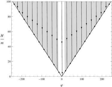
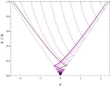
Figure 1: The black curves in the left plot are some numerically calculated (flat FLRW-$\varphi$) solutions, chosen so as to be evenly spaced in $\varphi$ at the early time $H=100m$, and with $\dot{\varphi}\geq 0$ at this early time (the solutions with $\dot{\varphi}\leq 0$ can be obtained by reflection). Only the behavior of $\varphi$ (horizontal axis) as a function of $H$ (vertical axis) is shown; the behavior of $a$ is not shown, as the $\varphi$ dynamics is independent of the value of $a$. A solution will undergo at least 60 $e$-folds of slow roll inflation if and only if it originates in one of the shaded regions. The right plot is a blow-up of the left plot near the origin. The solid curves are the solutions that have exited slow roll (i.e., they contain all the solutions drawn in the left plot, which are too close together at late times to distinguish on the plot) and the dashed curves are solutions that have never inflated.
     For the universes that undergo inflation, we see that $\varphi$ remains practically constant until $\dot{\varphi}$ reaches to the slow-roll value. Then the solution undergoes slow roll inflation along one of the diagonals (which are close to, but slightly offset from, the turning points $\varphi=\pm\sqrt{6}H/m$) until $H$ becomes small enough ($H_{f}\sim m$) and inflation ends. If we take the measure surface at an early time (large $H/m$), most of the solutions start out in the shaded region, but if we take the measure surface at a later time, a smaller fraction start out in the shaded region. As we discuss, this does not violate Liouville’s theorem, since solutions are “spreading out” in the other phase space dimension, $a$.

Although the measure of physical phase space is infinite, the range of $\varphi$ is bounded by (54) for any choice of $H_{*}$, so the infinity arises entirely from the unbounded range of $a$. Therefore, a very simple and natural way of “regularizing” the measure is to put in a cutoff, $a_{c}$, in $a$ and then take the limit as $a_{c}\rightarrow\infty$. Since the measure (53) factorizes in $\varphi$ and $a$ and the dynamics of $\varphi$ does not depend upon $a$, we obtain

$$P(N)=\lim_{a_{c}\rightarrow\infty}\frac{\,\displaystyle\left(\int_{0}^{a_{c}}a^{2}da\right)\left(\int_{\varphi_{i}\geq 2\sqrt{N}}\sqrt{6H_{*}^{2}-m^{2}\varphi^{2}\,}d\varphi\right)\,}{\,\displaystyle\left(\int_{0}^{a_{c}}a^{2}da\right)\left(\int_{0}^{\sqrt{6}\frac{H_{*}}{m}}\sqrt{6H_{*}^{2}-m^{2}\varphi^{2}\,}d\varphi\right)\,}\,,$$ (62)

where the $\varphi$-integral in the numerator is taken over the values of $\varphi$ at $H=H_{*}$ that come from trajectories with $\varphi\geq 2\sqrt{N}$ at $H=1$. Thus, we can simply cancel the integrals over $a$ and—after performing the $\varphi$-integral appearing in the denominator—we obtain the following well-defined formula for $P(N)$:

$$P(N)=\frac{2m}{3\pi H_{*}^{2}}\int_{\varphi_{i}\geq 2\sqrt{N}}\sqrt{6H_{*}^{2}-m^{2}\varphi^{2}\,}d\varphi\,.$$ (63)

By Liouville’s theorem (see section II), one might expect this expression to be independent of the choice of $H_{*}$. In fact, however, this expression is not independent of $H_{*}$. As we shall now show, if one evaluates $P(N)$ at $H_{*}\gg m$, one obtains a value very close to $1$ (in agreement with Carroll and Tam Carroll and Tam (2010)), whereas if one evaluates $P(N)$ at $H_{*}\sim m$ one obtains a value very close to $0$ (in agreement with Gibbons and Turok Gibbons and Turok (2008)). As we shall then explain, this strong $H_{*}$-dependence of (63) arises from the innocuous-looking regularization we performed in $a$.

Early-time evaluation ($H_{*}\gg m$): As can be seen from figure 1, $\varphi$ is nearly constant between $H=1$ and $H=H_{*}$ for trajectories that have not yet started inflation, so (63) reduces to

$$P(N) \approx\frac{2m}{3\pi H_{*}^{2}}\int_{2\sqrt{N}}^{\sqrt{6}\frac{H_{*}}{m}}\sqrt{6H_{*}^{2}-m^{2}\varphi^{2}\,}d\varphi$$ (64)

$$=\frac{4}{\pi}\int_{\zeta}^{1}\sqrt{1-x^{2}}dx$$

$$=\frac{2}{\pi}\left[\cos^{-1}\left(\zeta\right)-\zeta\sqrt{1-\zeta^{2}}\right]\,,$$

where $\zeta\equiv\sqrt{\frac{2m^{2}N}{3H_{*}^{2}}}$. For $\zeta\ll 1$, we can make the approximation

$$P(N)\approx 1-\frac{4}{\pi}\zeta\,.$$ (65)

For the choices $H_{*}=1/\sqrt{3}$ and $m=3\times 10^{-6}$ considered by Carroll and Tam Carroll and Tam (2010) , this expression yields $P(60)\approx 0.99996$, which agrees with their calculation.

Late-time evaluation ($H_{*}=H_{f}\sim m$): This choice of $H_{*}$ corresponds to the end of inflation for trajectories that have undergone inflation (see footnote 8). The slow roll approximation is no longer valid at this time, so the calculation can best be done by appealing to Liouville’s theorem and evaluating the phase space volume of interest at $H=1$. However, in order to apply Liouville’s theorem, we must return to the regulated expression (62), namely

$$P(N)=\lim_{a_{c}\rightarrow\infty}\frac{2m}{\pi H_{f}^{2}a_{c}^{3}}\int_{0}^{a_{c}}a^{2}da\int_{\varphi_{i}\geq 2\sqrt{N}}\sqrt{6H_{f}^{2}-m^{2}\varphi^{2}\,}d\varphi\,.$$ (66)

The joint integral over $a$ and $\varphi$ is just the GHS measure of the universes that underwent at least $N$ $e$-foldings of inflation and have $a\leq a_{c}$ when $H=H_{f}$. During the time before a trajectory starts inflating, the stress-energy tensor of $\varphi$ can be approximated by that of a perfect fluid with equation of state $p=\rho$ Hawking and Page (1988). During this period $a\propto t^{1/3}$, so $a\propto H^{-1/3}$, while $\varphi$ remains practically constant, $\varphi=\varphi_{i}$. Once $H$ becomes small enough, slow roll inflation will begin; by (55), the value of $H$ when inflation begins is

$$H_{s}\approx\frac{1}{\sqrt{6}}m\varphi_{i}\,.$$ (67)

Using (60), we then have

$$\frac{a\bigr{|}_{H=H_{f}}}{a\bigr{|}_{H=1}}=\frac{a\bigr{|}_{H=H_{f}}}{a\bigr{|}_{H=H_{s}}}\frac{a\bigr{|}_{H=H_{s}}}{a\bigr{|}_{H=1}}\approx e^{N}H_{s}^{-1/3}\approx e^{\varphi_{i}^{2}/4}\left(\frac{m\varphi_{i}}{\sqrt{6}}\right)^{-1/3}\,.$$ (68)

Thus, the condition $a\bigr{|}_{H=H_{f}}\leq a_{c}$ is approximately equivalent to the condition $a\bigr{|}_{H=1}<a_{c}\left(\frac{m\varphi_{i}}{\sqrt{6}}\right)^{1/3}e^{-\varphi_{i}^{2}/4}$. Thus, if we evaluate the GHS measure of the trajectories that we are considering at $H=1$, we obtain (neglecting overall numerical factors of order unity)

$$P(N) \propto\lim_{a_{c}\rightarrow\infty}\frac{1}{ma_{c}^{3}}\int_{2\sqrt{N}}^{\sqrt{6}/m}d\varphi\sqrt{6-m^{2}\varphi^{2}}\int_{0}^{a_{c}\left(\frac{m\varphi}{\sqrt{6}}\right)^{1/3}e^{-\varphi^{2}/4}}a^{2}da$$ (69)

$$\propto\int_{2\sqrt{N}}^{\sqrt{6}/m}d\varphi\sqrt{6-m^{2}\varphi^{2}}\,\varphi\,e^{-3\varphi^{2}/4}$$

$$\approx\int_{2\sqrt{N}}^{\sqrt{6}/m}d\varphi\sqrt{6\,}\,\varphi\,e^{-3\varphi^{2}/4}$$

$$\propto\left(e^{-3N}-e^{-9m^{2}/2}\right)$$

$$\approx e^{-3N}\,.$$

Note that the factors of $a_{c}$ canceled in the second line, so the expression is cutoff independent (and therefore there was no need to take the limit as $a_{c}\rightarrow\infty$ after that point). The dependence $P(N)\sim\exp(-3N)$ agrees with the results of Gibbons and Turok Gibbons and Turok (2008) and yields $P(N)\sim 10^{-80}$ for $N\sim 60$.

Thus, the situation with regard to obtaining the probability of inflation in minisuperspace using the GHS measure can now be seen to be closely analogous to that of obtaining the probability that an integer is even in the example given at the beginning of this section. In the integer example, one must first “regularize” the measure by imposing a “cutoff” that restricts one to subsets with finitely many integers. Similarly, in the minisuperspace case, one must first “regularize” the measure by putting in a “cutoff” in phase space that restricts one to subsets of finite volume. In the integer example, a natural cutoff can be imposed by ordering the integers by size and putting in a cutoff at $n$. Similarly, in the minisuperspace case, one can order the models by their “size”, $a$, at “time” $H_{*}$ and put in a cutoff at $a_{c}$. The difficulty is that the subsets of phase space with $a\leq a_{c}$ at “time” $H=H_{*}$ are very different in “shape” from the subsets of phase space with $a\leq a^{\prime}_{c}$ at “time” $H=H^{\prime}_{*}$. In particular, the universes with $a\leq a_{c}$ at an early time $H_{*}\gg m$ that will undergo inflation will be systematically “pushed out” to much larger values of $a$ at a late time $H_{*}\sim m$ than universes that do not inflate. Therefore if one regularizes by imposing a cutoff in $a$ at a late time, one will find that a much smaller percentage of universes will have inflated, as our calculations above explicitly show.

Should one impose a cutoff in $a$ at, say, the Planck time (see Corichi and Karami (2011)) and conclude that inflation is highly probable? Or, should one impose a cutoff in $a$ at a late time Turok (2011) and conclude that inflation is highly improbable? Or, should one impose an entirely different regularization scheme and perhaps draw an entirely different conclusion? Our purpose here is not to answer these questions but to emphasize that, even in this simple minisuperspace model, one needs more information than the GHS measure to obtain the probability of inflation.

V Contribution of Inhomogeneous Degrees of Freedom

In the previous section, we restricted our considerations to minisuperspace, i.e., the two dimensional submanifold of homogeneous, isotropic (FLRW) solutions. As discussed in section II, the pullback of the symplectic form to minisuperspace yields the GHS measure, which we used for the calculations of the previous section. However, minisuperspace is a set of measure zero in the full phase space. Even if we are only interested in “nearly FLRW” solutions, it is far from clear that the GHS measure will give a valid estimate of the phase space measure of the spacetimes that are “close” to a given FLRW solution. This difficulty is well illustrated by the following simple example (see figure 2): Consider the plane ${\bf R}^{2}$, with measure $\Omega=dxdy$, consider the line $y=0$ with measure $\Omega\bigr{|}_{y=0}=dx$, and consider the (union of the) yellow and red shaded regions. If we choose a point in the shaded regions of the plane “at random” with respect to the measure $\Omega$, we will find that it is more likely that the point lies in the red region than the yellow. But if we try to estimate this probability by choosing a point on the line “at random” with respect to the measure $\Omega\bigr{|}_{y=0}=dx$, we will get the wrong answer, i.e., we will find that it is more likely that it lies in the yellow region. It is quite possible that the situation for the phase space of general relativity could be quite similar: Specifically, the plane with measure $\Omega=dxdy$ could be analogous to the full phase space of general relativity with the measure of subsection II.2; the line $y=0$ with measure $\Omega\bigr{|}_{y=0}=dx$ could be analogous to minisuperspace with the GHS measure of subsection II.3; the (union of the) yellow and red shaded regions could be analogous to the spacetimes that, physically, are “close” to FLRW models; and the yellow and red regions could correspond to different properties of interest, e.g., the yellow region could correspond to universes that do not inflate, and the red region could correspond to universes that do. The minisuperspace calculation would then erroneously predict a low probability of inflation, since the full phase space calculation would give a high probability of inflation.

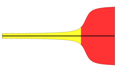
Figure 2: A region of the plane ${\bf R}^{2}$. The black line $y=0$ lies more in the yellow region than in the red region, but the red region is larger. In the “real” measure, $\Omega=dx\,dy$, a randomly chosen point is more likely to lie in the red region. But in the restricted measure, $\Omega\bigr{|}_{y=0}=dx$, a randomly chosen point is more likely to lie in the yellow region.

In this section, we will calculate the effects of including inhomogeneities on the measure of nearly FLRW models, thereby obtaining the modifications to the GHS measure produced by the type of effect illustrated in figure 2. Before presenting these calculations, however, we briefly discuss three significant difficulties of principle—for which we have no satisfactory resolutions—regarding the inclusion of inhomogeneous degrees of freedom, even when we restrict consideration to nearly FLRW models.

V.1 Difficulties Arising in the Treatment of Inhomogeneous Degrees of Freedom

The most serious difficulty arising in the treatment of inhomogeneous degrees of freedom is that there are infinitely many of them. As discussed in section II, in order to effectively reduce the system to a finite dimensional phase space, it is necessary to impose a short wavelength cutoff. There are obvious difficulties in imposing such a cutoff, since there is arbitrariness in the choice of cutoff, and, whatever choice is made, there undoubtedly will remain some coupling between the long wavelength degrees of freedom that are being kept, and the short wavelength degrees of freedom that are being discarded. However, in cosmology, there is an additional major issue of principle that arises from the fact that the physical wavelength of a mode is time dependent. In particular, if inflation occurs, a degree of freedom corresponding to a linearized perturbation of wavelength of order of the Planck scale at a time prior to inflation could correspond to a wavelength of order of the Hubble radius or larger in the present universe. If one imposes a short wavelength cutoff at a fixed physical scale such as the Planck scale, then the dimension of the phase space will vary with time, making it impossible to apply Liouville’s theorem or any usual statistical physics arguments. On the other hand, if one puts in a cutoff at a fixed co-moving wavelength so that the number of degrees of freedom does not change with time, then, in order to consider physically relevant degrees of freedom in the present universe, it may be necessary to consider degrees of freedom with wavelength smaller than the Planck length in the very early universe.

Another difficulty is that the notion of whether an inhomogeneous cosmology is “nearly FLRW” is a highly time dependent notion. Our own universe is believed to have been extremely homogeneous and isotropic on all scales during a much earlier phase, but is highly inhomogeneous on small scales now. On the other hand, most universes that are nearly homogeneous and isotropic at a Hubble constant corresponding to the present value, $H_{0}$, in our universe were extremely inhomogeneous at a much earlier phase Carroll and Tam (2010). Thus, the universes that are “nearly FLRW” at $H=H_{0}$ comprise a very different class of universes than those that are “nearly FLRW” at $H\gg H_{0}$.

Finally, even if we select a particular value, $H=H_{*}$, to impose a short wavelength cutoff and impose the requirement that inhomogeneities be “small,” it is not obvious how to define “smallness.” We will make such a choice in our calculations below, but one could argue that other choices are equally “natural,” and it is clear that the results will depend in a significant way upon the definition of “smallness.”

V.2 The Symplectic Form for Perturbations of FLRW

In section II.3 we evaluated the symplectic form of general relativity, $\omega[\chi;\delta_{1}\chi,\delta_{2}\chi]$, when $\delta_{1}\chi$ and $\delta_{2}\chi$ are homogeneous perturbations off an FLRW background $\chi$; the result of this calculation is given by (38). In this subsection, we will evaluate $\omega[\chi;\delta_{1}\chi,\delta_{2}\chi]$ when $\delta_{1}\chi$ and $\delta_{2}\chi$ are arbitrary (inhomogeneous) perturbations off of an FLRW background. This will enable us to obtain the Liouville measure on the space of “nearly-FLRW” universes, which we shall do in the next subsection.

We will mostly follow the notation of Mukhanov et al. Mukhanov et al. (1992) (although we use the opposite metric signature). In conformal time,

$$\eta=\int\frac{dt}{a}\,,$$ (70)

the metric of an FLRW universe takes the form

$$ds^{2}=a^{2}(\eta)\left(-d\eta^{2}+\gamma_{ij}dx^{i}dx^{j}\right)\,,$$ (71)

and the Friedmann equations take the form

$$\widetilde{H}^{2}+\kappa=\frac{1}{3}\left(\frac{1}{2}(\varphi_{0}^{\prime})^{2}+a^{2}V(\varphi_{0})\right)$$ (72)

$$\frac{a^{\prime\prime}}{a}+\kappa=-\frac{1}{3}\left(\frac{1}{2}(\varphi_{0}^{\prime})^{2}-2a^{2}V(\varphi_{0})\right)\,,$$ (73)

where ^′ denotes differentiation with respect to $\eta$, and

$$\widetilde{H}\equiv\frac{a^{\prime}}{a}=\dot{a}=aH\,.$$ (74)

We write,

$$\xi_{a}\equiv\nabla_{a}\eta\,,$$ (75)

and we define $D_{a}$ to be the derivative operator associated with $\gamma_{ab}$.

As is well known, there is a natural way to decompose any perturbation of an FLRW solution into its scalar, vector, and tensor parts Bardeen (1980); Mukhanov et al. (1992),

$$\delta g_{ab}=\left(\delta g_{ab}\right)_{\text{scalar}}+\left(\delta g_{ab}\right)_{\text{vector}}+\left(\delta g_{ab}\right)_{\text{tensor}}\,,$$ (76)

where

$$\left(\delta g_{ab}\right)_{\text{scalar}} = 2\,a^{2}\left(-\phi\xi_{a}\xi_{b}+\xi_{(a}D_{b)}B-\psi\gamma_{ab}+D_{a}D_{b}E\right)$$ (77)

$$\left(\delta g_{ab}\right)_{\text{vector}} = a^{2}\left(\xi_{(a}U_{b)}+D_{(a}V_{b)}\right)$$ (78)

$$\left(\delta g_{ab}\right)_{\text{tensor}} = a^{2}h_{ab}\,.$$ (79)

Here $U^{a}$ and $V^{a}$ are tangent to the spatial slices and are divergence free ($D_{a}U^{a}=D_{a}V^{a}=0$), whereas $h_{ab}$ is also tangent to the spatial slices, traceless ($h^{a}_{\phantom{a}a}=0$), and divergence free ($D^{a}h_{ab}=0$). In addition to the metric, we must also perturb the scalar field $\varphi$,

$$\varphi(\eta,x^{i})=\varphi_{0}(\eta)+\delta\varphi(\eta,x^{i})\,,$$ (80)

and $\delta\varphi$ is classified as belonging to the scalar part of the perturbation.

It is well known that the different perturbation types are decoupled in the linearized limit, i.e. the linearized Einstein equations break up into independent scalar, vector, and tensor pieces. The symplectic form, given by (23), is quadratic in the perturbations, but it is not difficult to see that the “cross terms” between the different perturbation types integrate to zero, so we have

$$\omega=\omega_{\text{scalar}}+\omega_{\text{vector}}+\omega_{\text{tensor}}\,,$$ (81)

where $\omega_{\text{scalar}}$ only contains terms quadratic in scalar perturbations, $\omega_{\text{vector}}$ only contains terms quadratic in vector perturbations, and $\omega_{\text{tensor}}$ only contains terms quadratic in tensor perturbations.

We will now calculate the scalar, vector, and tensor perturbation contributions to the symplectic form, $\omega$, and its pullback, $\overline{\omega}$, to the constraint submanifold.

V.2.1 Scalar Perturbations

Scalar perturbations naturally decompose into a “homogeneous part” (corresponding to perturbations towards other FLRW models) and an “inhomogeneous part” (for which the spatial integrals of $\phi$, $\psi$, and $\delta\varphi$ vanish). The computation of $\omega[\chi;\delta_{1}\chi,\delta_{2}\chi]$, when $\delta_{1}\chi$ and $\delta_{2}\chi$ are homogeneous perturbations was already done in section II.3. There are no cross terms in $\omega$ between homogeneous and inhomogeneous perturbations, so it remains only to calculate $\omega[\chi;\delta_{1}\chi,\delta_{2}\chi]$, when $\delta_{1}\chi$ and $\delta_{2}\chi$ are inhomogeneous perturbations.

From (77) and (80), we see that there are 5 scalar functions, $(\phi,\psi,B,E,\delta\varphi)$, defining an inhomogeneous scalar perturbation. However, there is gauge freedom to eliminate two of these functions via $\delta g_{ab}\rightarrow\delta g_{ab}+\nabla_{(a}v_{b)}$ with $v_{a}=\alpha\xi_{a}+D_{a}\beta$. Thus, there are three independent gauge-invariant variables Bardeen (1980), and we will use the choice of variables given in Mukhanov et al. (1992):

$$\Phi =\phi+\frac{1}{a}\left[a\left(B-E^{\prime}\right)\right]^{\prime}$$ (82)

$$\Psi =\psi-\frac{a^{\prime}}{a}(B-E^{\prime})$$

$$\sigma =\delta\varphi+\varphi_{0}^{\prime}(B-E^{\prime})\,.$$

In terms of these variables, the scalar linearized Einstein’s equations are Mukhanov et al. (1992)

$$D^{2}\Psi-3\widetilde{H}\left(\widetilde{H}\Phi+\Psi^{\prime}\right)+3\kappa\Psi=\frac{1}{2}\left[\varphi_{0}^{\prime}\left(\sigma^{\prime}-\varphi_{0}^{\prime}\Phi\right)+a^{2}\left.\frac{dV}{d\varphi}\right|_{\varphi_{0}}\sigma\right]$$ (83)

$$D_{i}\bigl{(}\widetilde{H}\Phi+\Psi^{\prime}-\frac{1}{2}\varphi_{0}^{\prime}\sigma\bigr{)}=0$$ (84)

$$\biggl{[}\Psi^{\prime\prime}+\widetilde{H}\left(\Phi^{\prime}+2\Psi^{\prime}\right)+\left(2\widetilde{H}^{\prime}+\widetilde{H}^{2}\right)\Phi-\kappa\Psi +\frac{1}{2}D^{2}(\Phi-\Psi)\biggr{]}\delta^{i}_{\phantom{i}j}-\frac{1}{2}D^{i}D_{j}(\Phi-\Psi)$$ (85)

$$=\frac{1}{2}\left[\left(\sigma^{\prime}-\varphi_{0}^{\prime}\Phi\right)\varphi_{0}^{\prime}-a^{2}\left.\frac{dV}{d\varphi}\right|_{\varphi_{0}}\sigma\right]\delta^{i}_{\phantom{i}j}$$

where spatial indices are raised by $\gamma^{ij}$, and $D^{2}\equiv D^{i}D_{i}$. Equation (85) implies that

$$\Phi=\Psi\,.$$ (86)

Plugging an FLRW solution and two inhomogeneous perturbations of the form (77, 80) into the formula, (23), for $\omega$, and using (82) and (86), we obtain

$$\omega_{\begin{subarray}{c}\text{scalar}\\ \text{inhom}\end{subarray}}=- 2a^{2}\int_{\Sigma}d^{3}x\sqrt{\gamma}\left\{3\Phi_{1}^{\prime}\Phi_{2}+\frac{1}{2}\left[4\varphi_{0}^{\prime}\Phi_{1}\sigma_{2}-\sigma_{1}^{\prime}\sigma_{2}\right]\right\}-(1\leftrightarrow 2)$$ (87)

$$+\left(\text{\small terms that vanish when the linearized Einstein equations are satisfied}\right)\,.$$

Here we have integrated by parts and dropped surface terms, since we are only considering universes with compact spatial slices. We have not explicitly written out the terms that vanish when the linearized Einstein equations are satisfied, since for the calculation of the Liouville measure, we will pull back the symplectic form to the constraint submanifold, and these terms will vanish. Note that, as we discussed in section II, the symplectic form should have “pure gauge” variations as its degeneracies when pulled back to the constraint surface; this can be seen explicitly in 87 since, when the linearized Einstein equations are satisfied, the non-vanishing terms have been written exclusively in terms of gauge invariant variables.

Using (83), (84), and (86) to eliminate $\sigma$ and $\sigma^{\prime}$ in terms of $\Phi$ and $\Phi^{\prime}$, we obtain

$$\omega_{\begin{subarray}{c}\text{scalar}\\ \text{inhom}\end{subarray}}=- \frac{4a^{2}}{(\varphi_{0}^{\prime})^{2}}\int_{\Sigma}d^{3}x\sqrt{\gamma}\Bigl{\{}\Phi_{1}^{\prime}\left(D^{2}+3\kappa\right)\Phi_{2}\Bigr{\}}-(1\leftrightarrow 2)$$ (88)

$$+\left(\text{\small terms that vanish when the linearized Einstein equations are satisfied}\right)\,.$$

We can further rewrite this expression by eliminating $\Phi^{\prime}$ in terms of the gauge invariant density contrast Carroll and Tam (2010)

$$\delta\equiv\frac{\delta\rho+\rho_{0}^{\prime}(B-E^{\prime})}{\rho_{0}}$$ (89)

where

$$\rho\equiv-\frac{1}{2}\nabla^{a}\varphi\nabla_{a}\varphi+V(\varphi)\,.$$ (90)

Using (83), we find that when the linearized Einstein equations hold, we have

$$\delta=\frac{2}{a^{2}\rho_{0}}\left[D^{2}\Phi-3\widetilde{H}\left(\widetilde{H}\Phi+\Phi^{\prime}\right)+3\kappa\Phi\right]\,.$$ (91)

We thereby obtain

$$\omega_{\begin{subarray}{c}\text{scalar}\\ \text{inhom}\end{subarray}} =\frac{2a\rho_{0}}{3H\dot{\varphi}_{0}^{2}}\int_{\Sigma}d^{3}x\sqrt{\gamma}\Bigl{\{}\delta_{1}\left(D^{2}+3\kappa\right)\Phi_{2}\Bigr{\}}-(1\leftrightarrow 2)$$ (92)

$$\qquad+\left(\text{\small terms that vanish when the linearized Einstein equations are satisfied}\right)\,,$$

where we have used (70) and (74) to switch from conformal time to proper time.

We can expand a general inhomogeneous perturbation in eigenfunctions of the Laplacian $D^{2}$ (which has a discrete spectrum since our spatial slices are compact). Let $f_{(n)}(x^{i})$ for $n=0,1,2,...$ satisfy

$$D^{2}f_{(n)}=-k_{n}^{2}f_{(n)}$$ (93)

with $k_{0}=0$ and $k_{n}$ nondecreasing in $n$, and

$$\int_{\Sigma}d^{3}x\sqrt{\gamma}f_{(m)}f_{(n)}=\delta_{n,m}\,,$$ (94)

where we remind the reader that we have normalized $\gamma_{ij}$ so that $\int_{\Sigma}d^{3}x\sqrt{\gamma}\equiv 1$. We expand

$$\Phi =\sum_{n=1}^{\infty}\Phi^{(n)}f_{(n)}$$ (95)

$$\delta =\sum_{n=1}^{\infty}\delta^{(n)}f_{(n)}\,.$$

Substituting these expansions into (92), pulling the expression back to the constraint submanifold, and adding in the homogeneous contribution $\omega_{\textsc{ghs}}$, we obtain

$$\overline{\omega}_{\text{scalar}}=\overline{\omega}_{\textsc{ghs}}+\sum_{n=1}^{\infty}\overline{\omega}_{\text{scalar}}^{(n)}\,,$$ (96)

where

$$\overline{\omega}_{\text{scalar}}^{(n)}=\frac{2a\rho_{0}\left(k_{n}^{2}-3\kappa\right)}{3H\dot{\varphi}_{0}^{2}}d\Phi^{(n)}\wedge d\delta^{(n)}=\frac{a\left(H^{2}+\kappa a^{-2}\right)\left(k_{n}^{2}-3\kappa\right)}{H\bigl{(}3H^{2}-V(\varphi_{0})+3\kappa a^{-2}\bigr{)}}d\Phi^{(n)}\wedge d\delta^{(n)}\,.$$ (97)

Finally, we comment that an irrotational fluid with equation of state $P=w\rho$ can be treated within our formalism by setting $V=0$ and replacing $X\equiv(-\frac{1}{2}\nabla^{a}\varphi\nabla_{a}\varphi)$ with $X^{\ell}$ in the Lagrangian (13), with $\ell=\frac{1+w}{2w}$. Carrying out the analogous calculations in the case $\kappa=0$, we obtain

$$\overline{\omega}_{\text{fluid}}^{(n)}=\frac{2k_{n}^{2}a\rho_{0}}{3H\left(\rho_{0}+p_{0}\right)}d\Phi^{(n)}\wedge d\delta^{(n)}\,.$$ (98)

This agrees with the expression obtained by Carroll and Tam Carroll and Tam (2010) for the case $p=\rho/3$.

V.2.2 Vector Perturbations

From (78), we see that there are two divergence-free spatial vectors, $U_{i}$ and $V_{i}$, defining a vector perturbation. However, there is gauge freedom to eliminate one of these vector fields via $\delta g_{ab}\rightarrow\delta g_{ab}+\nabla_{(a}v_{b)}$ with $v_{a}$ divergence free and tangent to the spatial slices. The combination

$$\overline{V}_{i}\equiv U_{i}-V_{i}^{\prime}$$ (99)

is gauge invariant Mukhanov (2005). One can calculate that the only term appearing in the integrand of $\omega_{\text{vector}}$ is proportional to $\left[(V_{1})^{i}D^{2}(\overline{V}_{2})_{i}-(1\leftrightarrow 2)\right]$. However, the constraint equation is Mukhanov (2005)

$$D^{2}\overline{V}_{i}=0\,,$$ (100)

where the right hand side is zero because the stress energy tensor has no vector part for scalar field matter. Thus, we have

$$\overline{\omega}_{\text{vector}}=0\,.$$ (101)

V.2.3 Tensor Perturbations

The tensor perturbation (79) involves a symmetric, traceless, and divergence-free spatial tensor field, $h_{ij}$. There are no constraints on $h_{ij}$ or its time derivative arising from Einstein’s equation, and $h_{ij}$ is gauge invariant. Plugging two tensor perturbations (79) into the formula (23) for the symplectic form, we obtain

$$\omega_{\text{tensor}}=-\frac{1}{4}a^{2}\int_{\Sigma}d^{3}x\sqrt{\gamma}\left((h_{1})_{ij}\frac{d(h_{2})^{ij}}{d\eta}-(1\leftrightarrow 2)\right)\,.$$ (102)

Let $\left(f_{(n)}\right)_{ij}$ for $n=1,2,...$ denote an orthonormal basis of divergence free and traceless eigentensors of $D^{2}$, i.e.,

$$D^{2}\left(f_{(n)}\right)_{ij}=-\widetilde{k}_{n}^{2}\left(f_{(n)}\right)_{ij}\,,$$ (103)

with $\widetilde{k}_{n}$ nondecreasing in $n$, and

$$\int_{\Sigma}d^{3}x\sqrt{\gamma}\left(f_{(n)}\right)_{ij}\left(f_{(m)}\right)^{ij}=\delta_{n,m}\,$$ (104)

(we remind the reader that spatial indices are raised by $\gamma^{ij}$). We expand

$$h_{ij}=\sum_{n=1}^{\infty}h^{(n)}(\eta)\left(f_{(n)}\right)_{ij}\,.$$ (105)

(Note that we are including both polarizations in the sum.) We obtain

$$\omega_{\text{tensor}}=-\frac{1}{4}\,a^{2}\sum_{n=1}^{\infty}dh^{(n)}\wedge d\left(h^{(n)}\right)^{\prime}=\frac{1}{4}\,a^{3}\sum_{n=1}^{\infty}d\dot{h}^{(n)}\wedge dh^{(n)}\,.$$ (106)

The formula for $\overline{\omega}_{\text{tensor}}$ is identical, as there are no tensor constraints.

V.3 Modifying the GHS Measure by Including Inhomogeneities, and the Effect on the Probability of Inflation

As discussed is section II, in order to obtain a finite dimensional phase space, we impose a short wavelength cutoff. We do so by discarding all scalar modes that have $n>\mathcal{N}_{1}$ and all tensor modes that have $n>\mathcal{N}_{2}$. (Note that if we put the cutoffs at approximately the same values of wavelength, i.e., if $k^{2}_{\mathcal{N}_{1}}\approx\widetilde{k}^{2}_{\mathcal{N}_{2}}$, then we will have $\mathcal{N}_{2}\sim 2\mathcal{N}_{1}$, since there are two tensor polarizations.) Imposing these cutoffs and combining (96) with (106), we obtain the following expression for the symplectic form for perturbations of FLRW, pulled back to the constraint surface:

$$\overline{\omega}=\overline{\omega}_{\textsc{ghs}}+\frac{2a\rho_{0}}{3H\dot{\varphi}_{0}^{2}}\sum_{n=1}^{\mathcal{N}_{1}}\left(k_{n}^{2}-3\kappa\right)d\Phi^{(n)}\wedge d\delta^{(n)}+\frac{1}{4}\,a^{3}\sum_{n=1}^{\mathcal{N}_{2}}d\dot{h}^{(n)}\wedge dh^{(n)}\,.$$ (107)

As discussed in section II, to obtain a nondegenerate symplectic form, we further restrict to the surface $\mathcal{S}$ defined by $K=3H_{*}$, i.e., we impose $H=H_{*}$ on the background FLRW spacetime and $\delta K=0$ on the perturbations. In addition, as mentioned in II.2, we must fix the spatial coordinates as well. However, our variables describing inhomogeneous perturbations have been written in a gauge invariant form, so there is no change in their functional form when we restrict to $\delta K=0$ and fix spatial coordinates. Furthermore, homogeneous spatial diffeomorphisms act trivially on the homogeneous perturbations. Thus, we obtain

$$\omega\bigr{|}_{\mathcal{S}} =\left(\frac{3a^{2}\left(6H_{*}^{2}-m^{2}\varphi^{2}+4\kappa a^{-2}\right)}{\sqrt{6H_{*}^{2}-m^{2}\varphi^{2}+6\kappa a^{-2}}}\right)d\varphi\wedge da$$ (108)

$$\quad+\frac{a\left(H_{*}^{2}+\kappa a^{-2}\right)}{H_{*}\bigl{(}3H_{*}^{2}-V(\varphi_{0})+3\kappa a^{-2}\bigr{)}}\sum_{n=1}^{\mathcal{N}_{1}}\left(k_{n}^{2}-3\kappa\right)d\Phi^{(n)}\wedge d\delta^{(n)}$$

$$\quad+\frac{1}{4}\,a^{3}\sum_{n=1}^{\mathcal{N}_{2}}d\dot{h}^{(n)}\wedge dh^{(n)}\,,$$

where we have used the explicit form of the GHS measure, (46), derived in section II.3.

To obtain the Liouville measure on our truncated, $2(1+\mathcal{N}_{1}+\mathcal{N}_{2})$-dimensional phase space, we take the top exterior product of $\omega\bigr{|}_{\mathcal{S}}$, thereby obtaining

$$\Omega\equiv \frac{1}{(1+\mathcal{N}_{1}+\mathcal{N}_{2})!}\wedge^{(1+\mathcal{N}_{1}+\mathcal{N}_{2})}\omega\bigr{|}_{\mathcal{S}}$$ (109)

$$=\left(\frac{3a^{2}\left(6H_{*}^{2}-m^{2}\varphi^{2}+4\kappa a^{-2}\right)}{\sqrt{6H_{*}^{2}-m^{2}\varphi^{2}+6\kappa a^{-2}}}\right)d\varphi\wedge da$$

$$\quad\wedge\left(\frac{a\left(H_{*}^{2}+\kappa a^{-2}\right)}{H_{*}\bigl{(}3H_{*}^{2}-V(\varphi_{0})+3\kappa a^{-2}\bigr{)}}\right)^{\mathcal{N}_{1}}\prod_{n=1}^{\mathcal{N}_{1}}\left(k_{n}^{2}-3\kappa\right)d\Phi^{(n)}\wedge d\delta^{(n)}$$

$$\quad\wedge\left(\frac{1}{4}\,a^{3}\right)^{\mathcal{N}_{2}}\prod_{n=0}^{\mathcal{N}_{2}}d\dot{h}^{(n)}\wedge dh^{(n)}\,.$$

This expression for the $2(1+\mathcal{N}_{1}+\mathcal{N}_{2})$-form $\Omega$ is, of course, valid only when evaluated at exact FLRW models. However, if we restrict consideration to solutions that are sufficiently close to FLRW models, we should be able to neglect the dependence of $\Omega$ on $(\Phi^{(1)},\delta^{(1)},\dots,\Phi^{(\mathcal{N}_{1})},\delta^{(\mathcal{N}_{1})},\dot{h}^{(1)}h^{(1)},\dots,\dot{h}^{(\mathcal{N}_{2})}h^{(\mathcal{N}_{2})})$ and continue to use (109) to calculate phase space volumes of regions sufficiently near FLRW models.

We now wish to integrate $\Omega$ over a range of perturbation variables corresponding to “small inhomogeneities,” so as to obtain the “true” measure of nearly FLRW spacetimes (see figure 2 and the associated discussion at the beginning of this section). To do so, we need to decide how to define “small inhomogeneities”, i.e., how to choose which universes are “nearly FLRW”. Following Carroll and Tam Carroll and Tam (2010), we will choose the variables $\Phi$ and $\delta$ to indicate the “size” of scalar perturbations, since $|\Phi|\ll 1$ means that the metric perturbation is small compared to the background metric, and $|\delta|\ll 1$ means that the density perturbation is small compared to the background density. For the tensor perturbations, we will choose $h$ and $\dot{h}/H$ as indicators of “size,” since $|h|\ll 1$ means the metric perturbation is small, and $|\dot{h}|\ll H$ means that the perturbation of the extrinsic curvature is small compared to the background. Thus, we provisionally define “nearly FLRW” universes at “time” $H_{*}$ to be those that have $|\Phi(H=H_{*})|\leq\epsilon$, $|\delta(H=H_{*})|\leq\epsilon$, $|h(H=H_{*})|\leq\epsilon$, and $|\dot{h}(H=H_{*})|\leq H_{*}\epsilon$ for some $\epsilon>0$. (Here, for simplicity, we have taken $\epsilon$ to be independent of $n$ and the same for scalar and tensor modes.) Then, the modified GHS measure on minisuperspace, which takes the “thickening” effects of inhomogeneities into account, is given by

$$\widetilde{\Omega}_{\textsc{ghs}} \equiv\int\limits_{\begin{subarray}{c}|\Phi^{(n)}|\leq\epsilon\\ |\delta^{(n)}|\leq\epsilon\\ |h^{(n)}|\leq\epsilon\\ |{\dot{h}}^{(n)}|\leq\epsilon H_{*}\\ \end{subarray}}{\Omega}\quad$$ (110)

$$=\,\left(\frac{4\epsilon^{2}a\left(H_{*}^{2}+\kappa a^{-2}\right)}{H_{*}\bigl{(}3H_{*}^{2}-V(\varphi_{0})+3\kappa a^{-2}\bigr{)}}\right)^{\mathcal{N}_{1}}\cdot\left(\prod_{n=1}^{\mathcal{N}_{1}}\left(k_{n}^{2}-3\kappa\right)\right)\cdot\left(\epsilon^{2}a^{3}H_{*}\right)^{{\mathcal{N}_{2}}}\cdot\Omega_{\textsc{ghs}}\,,$$

where $\Omega_{\textsc{ghs}}$ is given by equation (46). For the case of $\kappa=0$ and $V(\varphi)=\frac{1}{2}m^{2}\varphi^{2}$, and choosing $\mathcal{N}_{2}=2\mathcal{N}_{1}\equiv 2\mathcal{N}$, we obtain

$$\widetilde{\Omega}_{\textsc{ghs}}\propto\left(\frac{a^{7}H_{*}^{3}}{6H_{*}^{2}-m^{2}\varphi_{0}^{2}}\right)^{\mathcal{N}}\Omega_{\textsc{ghs}}=\left(\frac{a^{7}H_{*}^{3}}{6H_{*}^{2}-m^{2}\varphi_{0}^{2}}\right)^{\mathcal{N}}\sqrt{6H_{*}^{2}-m^{2}\varphi_{0}^{2}\,}\,a^{2}dad\varphi_{0}\,.$$ (111)

Note that $\widetilde{\Omega}_{\textsc{ghs}}$ varies with $a$ as $a^{2+7\mathcal{N}}$, so including more perturbation modes makes the large-$a$ divergence more severe. In particular, including the effect of perturbations on the measure does not alleviate the difficulties discussed in section IV associated with the infinite total measure of minisuperspace.

It is easily seen that $\widetilde{\Omega}_{\textsc{ghs}}$ has a non-integrable divergence (for $\mathcal{N}\geq 2$) as $\varphi_{0}\rightarrow\pm\sqrt{6}H_{*}/m$, which lies at the boundary of the range of $\varphi_{0}$ allowed by the Hamiltonian constraint (50), and corresponds to $\dot{\varphi}_{0}\rightarrow 0$. The origin of this divergence can be traced to the fact that $\Phi^{(n)}$ and $\delta^{(n)}$ become linearly dependent at $\varphi_{0}=\pm\sqrt{6}H_{*}/m$. Thus, as $\varphi_{0}\rightarrow\pm\sqrt{6}H_{*}/m$, a box of “size” $\epsilon$ in $\Phi^{(n)}$ and $\delta^{(n)}$ allows an unboundedly large range of other variables such as

$$\dot{\sigma}^{(n)}\approx\frac{m^{2}\varphi_{0}}{H_{*}\dot{\varphi}_{0}^{2}}\left(\frac{m^{2}\varphi_{0}^{2}}{6}\delta^{(n)}+\frac{2k_{n}^{2}}{3a^{2}}\Phi^{(n)}\right)\,,$$ (112)

where $\sigma$ was defined by (82). We will therefore supplement our definition of “nearly FLRW” universes by imposing the additional requirement that $|\dot{\sigma}^{(n)}|\ll m|\varphi_{0}|$ when $\dot{\varphi}_{0}$ is close to zero. This eliminates the divergence at $\varphi_{0}\rightarrow\pm\sqrt{6}H_{*}/m$ that occurs in (111) without affecting our formula for the measure when $\varphi_{0}$ is not close to $\pm\sqrt{6}H_{*}/m$.

Let us now compute the probability of inflation in parallel with the analysis of section IV, but using the measure $\widetilde{\Omega}_{\textsc{ghs}}$ rather than $\Omega_{\textsc{ghs}}$. First, we perform an “early-time evaluation” ($H_{*}\gg m$) of the probability of inflation. For fixed $a$, the GHS measure is peaked at $\varphi_{0}=0$ and decreases to zero as $\varphi_{0}$ approaches the boundary of its allowed range, so the GHS measure is peaked on universes that have the least amount of inflation. By contrast, $\widetilde{\Omega}_{\textsc{ghs}}$ is more peaked near the boundary of the allowed range of $\varphi_{0}$, where the most inflation occurs. Thus, the probability of inflation computed using $\widetilde{\Omega}_{\textsc{ghs}}$ at early times will be even higher than the (extremely high) value obtained in section IV using $\Omega_{\textsc{ghs}}$.

On the other hand, suppose we perform a late-time evaluation ($H_{*}\sim m$) of the probability of inflation. In this case, the main effect of including the perturbation modes comes from the change in the $a$ dependence of the measure from $\Omega_{\textsc{ghs}}\propto a^{2}$ to $\widetilde{\Omega}_{\textsc{ghs}}\propto a^{2+7\mathcal{N}}$. Carrying out the analysis in parallel with section IV, we obtain

$$P(N)\sim e^{-(3+7\mathcal{N})N}\,,$$ (113)

which is much smaller than the (extremely small) probability of inflation calculated in section IV using $\Omega_{\textsc{ghs}}$.

As in section IV, our purpose here is not to advocate for performing the calculations at early times or at late times, nor to advocate for our particular choice of definition of “nearly FLRW” spacetimes. Rather, our purpose is merely to illustrate in a concrete manner the additional issues that arise—and the additional choices that need to be made—when one takes the inhomogeneous degrees of freedom into account.

VI Impossibility of Retrodiction

In the previous sections, we have highlighted difficulties that arise when one attempts to use the natural Liouville measure of general relativity to calculate probabilities in cosmology, such as the probability of inflation. Some of the difficulties are a direct consequence of the fact that the measure of phase space is infinite. A possible approach to dealing with this problem is to use our knowledge of (or beliefs about) the present universe to reduce the relevant region of phase space to one that has finite volume. In particular, we know/believe that the present universe is nearly an FLRW model. We do not know the present value of the scalar factor, $a$, of this background FLRW model, but we can simply assume that it takes some particular value $a_{0}$. Suppose we restrict consideration to the region, $A$, of phase space corresponding to universes that differ by a suitably small (but finite) amount from this background FLRW model at the time when the trace of the extrinsic curvature is equal to the present value, $H_{0}$, of the Hubble constant. If we let $B$ denote the subset of universes that undergo suitably many $e$-foldings of inflation, then one might argue that—taking account of our knowledge of the present state of the universe—the probability that our universe underwent an era of inflation should be given by

$$P=\frac{\Omega(B\cap A)}{\Omega(A)}\,,$$ (114)

where $\Omega$ is the canonical measure of general relativity, and the right side is now well defined, since $A$ and $B\cap A$ have finite measure. Indeed, this formula essentially corresponds to the calculation of the previous subsection taking $H_{*}=H_{0}$; a calculation of this nature was also carried out in Carroll and Tam (2010). We refer to this type of calculation as a “retrodiction” because it uses present conditions as an input to determine the likelihood of past conditions. The purpose of this section is to argue that, in a universe in which the second law of thermodynamics is valid, this type of calculation is essentially guaranteed to give the wrong answer, i.e., it will assign an extremely low probability to what actually did happen in the past. This “futility of retrodiction” has been discussed in depth by Eckhardt Eckhardt (2006), and we refer the reader to that reference for additional discussion.

In ordinary statistical mechanics, we can use knowledge about the present macrostate of a system to successfully predict the likely future evolution of the system. This is done by considering all of the possible microstates that are consistent with the present macrostate and evolving them forward in time using the (microscopic) dynamical equations. If it is found that an overwhelming majority (in the Liouville measure) of these microstates will have some given property at some specified time in the future, then we can be confident in predicting that the physical system will have that property at that specified time. We refer to this type of argument as a “trajectory counting argument”. The key point is that although one can use a trajectory counting argument to predict the future, one cannot use a trajectory counting argument to “retrodict” the past. The time reversal invariance of the microscopic dynamics assures us that most trajectories through phase space that pass through a present non-equilibrium macrostate have entropy that is increasing both into the future and into the past. However, it appears that we live in a universe in which the second law of thermodynamics holds, where entropy increases only in one time direction (“the future”). In practice, we find that trajectory counting arguments do give correct results when used to make predictions; i.e., systems do not appear to be evolving towards some “special final state.” However, because entropy in our universe decreases towards the past, trajectory counting arguments will always give incorrect answers when used to make retrodictions.

A simple example will illustrate this point. Suppose that at 12:00 there is a cup of water with a temperature slightly above freezing and with a small ice cube floating in it. It is known that the cup was isolated since at least 11:59, and it will remain isolated until at least 12:01. Was there a larger ice cube at 11:59? A trajectory counting argument for this case would consider all possible histories that have a small ice cube in the cup at 12:00 and calculate the fraction (in the Liouville measure) of those histories for which there is a larger ice cube in the cup at 11:59. Very few trajectories have this property; the overwhelming majority have a smaller ice cube (or only liquid water) at 11:59. Indeed, since this system is time reversal invariant, the trajectory counting argument will give the same answer whether we go forward or backward in time. The trajectory counting argument will correctly predict that there will be less ice by 12:01. It will incorrectly retrodict that there was less ice at 11:59.

The same behavior applies in cosmology. If, as above, we let $A$ be the set of universes that can be described as “nearly-FLRW today,” then most universes in $A$ were extremely inhomogeneous at early times Carroll and Tam (2010). Indeed, if we consider almost any universe that looks like ours now and reverse-evolve it into the past, we would find that inhomogeneities would generically grow (into the past)—so much that they could no longer be described by the linearized theory. Inflation (or, “deflation,” since we are evolving backwards) would surely not occur at early times. In other words, in the set of all possible histories that are consistent with our current conditions, the most numerous type of history (in the Liouville measure) is one in which the universe was highly inhomogeneous in the past—with many regions of “delayed big bangs,” i.e., “white holes”—and just managed to smooth itself out enough by our present time so that it could be approximately described today as a linear perturbation of FLRW.

As we have just argued, in a universe in which the second law of thermodynamics holds, we cannot test a hypothesis about the past by retrodiction, i.e., we cannot test it by determining whether the hypothesized occurrence is generic in the space off all possible histories consistent with present observation. Rather, to ascertain what happened in the past, we make hypotheses about the past based on considerations such as simplicity (à la “Occam’s Razor”) and mathematical elegance. Once we have made such a hypothesis, we can test it using prediction rather than retrodiction. If a simple and/or elegant hypothesis about the past makes predictions—via trajectory counting arguments—that are in agreement with observation, this is taken as evidence in favor of the hypothesis. The simpler and more elegant the hypothesis and the more it accounts for, the stronger we consider the evidence in its favor. In a universe in which the second law of thermodynamics is obeyed, this is essentially the only way to get information about the past state. For example, we deduce that light element nucleosynthesis must have occurred in the early universe not by taking the nuclear abundances of the present universe and retrodicting past de-synthesis, but by making very simple hypotheses about the state of the early universe and predicting the abundances we see today. The evidence for light element nucleosynthesis is strong because much is explained from a simple hypothesis.

In a similar manner, we assert that if one wishes to make an argument in favor of inflation having occurred in the early universe, this argument must be based upon its being a simple and/or elegant hypothesis that accounts for observed phenomena. Any argument about the “likelihood” of inflation based upon the Liouville (or other) measure on phase space will require a justification for the use of this measure (see section III) as well as a justification for the regularizations used to obtain probabilities from this measure (see sections IV and V). Furthermore, as we have argued in this section, we cannot obtain any useful information about whether inflation occurred in the early universe by determining whether it is generic in the space of all universes that look like ours today.