Virtual Parallel Computing and a Search Algorithm using Matrix Product States

Abstract

We propose a form of parallel computing on classical computers that is based on matrix product states. The virtual parallelization is accomplished by representing bits with matrices and by evolving these matrices from an initial product state that encodes multiple inputs. Matrix evolution follows from the sequential application of gates, as in a logical circuit. The action by classical probabilistic one-bit and deterministic two-bit gates such as NAND are implemented in terms of matrix operations and, as opposed to quantum computing, it is possible to copy bits. We present a way to explore this method of computation to solve search problems and count the number of solutions. We argue that if the classical computational cost of testing solutions (witnesses) requires less than $O(n^{2})$ local two-bit gates acting on $n$ bits, the search problem can be fully solved in subexponential time. Therefore, for this restricted type of search problem, the virtual parallelization scheme is faster than Grover’s quantum algorithm.

Interference and the ability to follow many history paths simultaneously make quantum systems attractive for implementing computations deutsch85 . Efficient algorithms exploring these properties have been proposed to solve practical problems such as number factoring shor94 and unsorted database search grover97 . However, we still do not have a sufficiently large and resilient quantum computer to take advantage of these algorithms. It is, thus, very desirable to try to find better and more efficient ways to compute with classical systems. In this regard, recent advances in our understanding of quantum many-body systems provide some guidance. It is well understood now that the time evolution of a large class of one-dimensional interacting systems can be efficiently simulated by expressing their wave functions in a matrix product state form and by using a time-evolving block decimation (TEBD) vidal . A key aspect of this success is data compression: even though many-body interactions tend to increase the rank of the matrices over time, it is possible to use truncation along the evolution to keep the matrices relatively small, such that the resulting wave function approximates quite accurately the exact one without an exponential computation cost verstraete2008 . In quantum systems, it is well understood that local interactions do not quickly entangle one-dimensional many-body state, justifying the matrix truncation cirac2009 ; hamma2011 .

In this Letter, we describe a method of classical computation that utilizes matrix product states (MPS) to implement search and other similar tasks. Compression, when possible, provides additional speedup. Formally, instead of working with wave functions and quantum amplitudes, we describe the state of the computer in terms of a stochastic probability distribution written as traces of matrix product states associated to bit configurations. The idea of expressing classical probability distributions in the form of MPS is not new derrida1993 , but the focus so far has been on using it to study nonequilibrium phenomena of physical systems (see for instance Ref. temme2010, ; johnson2010, ). As we show below, a MPS formulation of classical probability distributions can also be employed to create a virtual parallel machine where all possible outcomes of an algorithm are obtained for all $2^{n}$ inputs of an $n$-bit register. Information about these outcomes is encoded and compressed in the matrices forming the MPS. By itself this “parallelism” is not obviously useful; it is, however, if a certain problem can use the probability of a single outcome at a time. This is the case of a search problem that seeks, for a given $y$, the value of $x$ such that $y=f(x)$ for an algorithmically computable function $f$. Then, the focus is not on all values of the output, but on only one given $y$. We shall show below that in this case matrix computing can be useful. In particular, from the probability of $y$, the method directly provides the number of input values $x$ satisfying the functional constraint $y=f(x)$.

In our matrix computing, insertion and removal of bits are allowed and one-bit and two-bit gates can be implemented much like in a conventional computer. Our one-bit gates are probabilistic while our two-bit gates are deterministic. Two-bit gates rely on a singular value decomposition (SVD) to maintain the MPS form of the probability distribution. All these operations preserve the positivity and the overall normalization of the probability even though we work with nonpositive matrices.

Matrix computing formulation – Consider a set of binary variables $\{x_{j}=0,1\}_{j=1,\ldots,n}$ describing a set of $n$ bits, with $|x_{1}\,x_{2}\ldots x_{n}\rangle\equiv|x\rangle$ denoting a particular configuration of this system. In analogy to quantum mechanics, we define the vector

$$|P\rangle=\sum_{x_{n},\ldots,x_{1}=0,1}P(x_{1},\ldots,x_{n})\,|x_{1}\ldots x_{n}\rangle,$$ (1)

where

$$P(x_{1},\ldots,x_{n})=\mbox{tr}\left(M_{1}^{x_{1}}\cdots M_{n}^{x_{n}}\right).$$ (2)

Here, each $M_{j}^{x_{j}}$ is a real matrix of dimensions $D_{j-1}\times D_{j}$. The trace can be dropped if we consider the first and last matrices to be row and column vectors, i.e., $D_{0}=D_{n}=1$. The state vector is normalized in the following sense: define $|\Sigma\rangle=\sum_{x_{1},\ldots,x_{n}=0,1}|x_{1}\ldots x_{n}\rangle$, then $Z=\langle\Sigma|P\rangle=1$ since $\sum_{x}P(x)=1$.

Starting from an initial probability distribution $P_{0}(x_{1},\ldots,x_{n})$, the vector $|P\rangle$ evolves as a sequence of one-bit and nearest-neighbor two-bit gates is applied to the bit matrices. These bit operations form a logical circuit, which is tailored according to a particular computational problem, for instance, the algorithmic computation of a function $f(x)$. Below, we describe how bit operations are implemented.

$\bullet$ One-bit gates: We will use probabilistic one-bit gates, which take states $0,1$ to states $0,1$ with probabilities $p,1-p$ and $q,1-q$:

$$0\xrightarrow{\;\;p\;\;}0\quad{\rm or}\quad 0\xrightarrow{1-p}1$$

$$1\xrightarrow{1-q}0\quad{\rm or}\quad 1\xrightarrow{\;\;q\;\;}1\;.$$

The probabilities can be encoded into a transfer function $t^{\tilde{a},a}$ that takes a logic input $a=0,1$ into a logic output $\tilde{a}=0,1$. Explicitly: $t^{0,0}=p$, $t^{1,0}=1-p$, $t^{0,1}=1-q$, $t^{1,1}=q$. A one-bit gate acting on bit $j$ yields a new matrix

$$\tilde{M}_{j}^{x_{j}}=\sum_{x^{\prime}_{j}=0,1}t^{x_{j},x^{\prime}_{j}}\;M_{j}^{x^{\prime}_{j}}\;.$$ (3)

The transfer function satisfies the sum rule $\sum_{{\tilde{a}}=0,1}t^{\tilde{a},a}=1$, which ensures that the normalization $Z=1$ is maintained as the system evolves. Examples of one-bit gates are: (a) Deterministic NOT, with $p=0$ and $q=0$, (b) RAND, with $p=1/2$ and $q=1/2$, which randomizes the bit, (c) RST, with $p=1$ and $q=0$, which resets the bit to 0.

$\bullet$ Two-bit gates: We will consider only deterministic two-bit gates. Given two logical functions $A(a,b)$ and $B(a,b)$, we construct the transfer function $T^{\tilde{a}\tilde{b},ab}$, taking bits with states $a$ and $b$ to bits with states $\tilde{a}$ and $\tilde{b}$, respectively:

$$T^{\tilde{a}\tilde{b},ab}=\begin{cases}1,&\text{$\tilde{a}=A(a,b)$\ and\ $\tilde{b}=B(a,b)$},\\ 0,&\text{otherwise}.\end{cases}$$ (4)

Similarly to one-bit gates, the normalization after two-bit gates is preserved by the sum rule $\sum_{{\tilde{a}},{\tilde{b}}=0,1}T^{\tilde{a}\tilde{b},ab}=1$. The evolved matrices must satisfy

$$\;\tilde{M}_{j-1}^{x_{j-1}}\,\tilde{M}_{j}^{x_{j}}=\sum_{x^{\prime}_{j-1},x^{\prime}_{j}=0,1}T^{x_{j-1}x_{j},x^{\prime}_{j-1},x^{\prime}_{j}}\,M_{j-1}^{x^{\prime}_{j-1}}\;M_{j}^{x^{\prime}_{j}},$$ (5)

and we use the SVD to decompose the result of the gate operation on the right-hand side of Eq. (5) as a product of two matrices, as in the left-hand side of the equation, for all the four cases $x_{j-1},x_{j}=0,1$.

Let us demonstrate this construction with a concrete example. Consider the following logical operation on bits $j-1$ and $j$: $A_{\rm NAND}(a,b)=a$ and $B_{\rm NAND}(a,b)=\overline{a\land{}b}$. The first bit is unaffected, while the second one evolves into the NAND operation between the two bits. In this case, $T^{01,00}=T^{01,01}=T^{11,10}=T^{10,11}=1$, with all other elements set to zero. We use the transfer function to determine the four blocks (for $x_{j-1},x_{j}=0,1$) of a matrix ${\cal M}^{\rm NAND}_{j-1,j}$ of dimension $2D_{j-2}\times 2D_{j}$:

$${\cal M}^{\rm NAND}_{j-1,j}=\left(\begin{array}[]{c|cc}0&M_{j-1}^{0}M_{j}^{0}+M_{j-1}^{0}M_{j}^{1}\\ \\ \hline\cr\\ M_{j-1}^{1}M_{j}^{1}&M_{j-1}^{1}M_{j}^{0}\end{array}\right).$$ (6)

To factor the matrix ${\cal M}_{j-1,j}$ back into a product, we employ an SVD,

$${\cal M}_{j-1,j}\stackrel{{\scriptstyle\rm SVD}}{{=}}\left(\begin{array}[]{c}\tilde{M}_{j-1}^{0}\\ \\ \tilde{M}_{j-1}^{1}\end{array}\right)\left(\begin{array}[]{cc}\tilde{M}_{j}^{0}&\tilde{M}_{j}^{1}\end{array}\right).$$ (7)

In this process, the common dimension $D_{j-1}$ may change and likely increase. This is an issue of fundamental important, which we shall return when we discuss a search algorithm.

$\bullet$ Bit insertions and removals: For computational tasks such addition and multiplication, it is important to be able to insert and remove bits. These operations are straightforward for MPS. Insertion of a new bit (say, initially set to 0) in between bits $j-1$ and $j$ amounts to replacing $M_{j-1}^{x_{j-1}}M_{j}^{x_{j}}$ with $M_{j-1}^{x_{j-1}}M_{\alpha}^{x_{\alpha}}M_{j}^{x_{j}}$, where $M_{\alpha}^{1}$ and $M_{\alpha}^{0}$ are $D_{j-1}\times D_{j-1}$ null and identity matrices, respectively, and the total sum over bit configurations in the vector $|P\rangle$ [see Eq. (1)] has now to include the binary variable $x_{\alpha}=0,1$. Removal of a bit is done by absorbing its matrix into the one of an adjacent bit, namely, by tracing it out; for instance, we use $\sum_{x_{j}=0,1}M_{j}^{x_{j}}M_{j+1}^{x_{j+1}}=\tilde{M}_{j+1}^{x_{j+1}}$ to remove bit $j$.

How can matrix computing be used to solve certain computational problems? – Here we shall present computational algorithms that explore the virtual parallelism encoded in matrix product states. To be concrete, consider the following search problem as an example:

• Given a function $y=f(x)$ that can be computed algorithmically with $O(n^{d})$ gates and a certain value for $y$, we would like to search for an input $x$ that yields as output $y=f(x)$.

The reason why matrix computation is useful for this search problem can be argued as follows. Matrix product states can express the probability values of all possible $m$-bit outputs $y\equiv y_{1}\,y_{2}\dots y_{m}$ if one starts with a product state encoding all possible $n$-bit inputs $x\equiv x_{1}\,x_{2}\dots x_{n}$, namely, $P(x)=2^{-n}$ for all $x$. Of course, if we were interested in all the probabilities, we would have to compute an exponentially large ($2^{m}$) number of traces of products of matrices. But this is not what is needed to perform the search above: we are interested in just one output $y$ for this problem. We, thus, proceed in the following steps.

1. Starting with all bits $x_{i}$, $i=1,\dots,n$, randomized with equal probabilities $1/2$ for being $0$ or $1$, we compute the final output matrices $M_{j}^{y_{j}}$, $j=1,\ldots,m$, resulting from the action of the circuit that evaluates $f(x)$.

2. We compute the probability $P(y)$ for the given $y$ we are interested in. If $P(y)\geq 2^{-n}$, then there is at least one value of $x$ such that $y=f(x)$.

3. We then fix one of the input bits, say $x_{1}$, to be $0$, instead of randomizing it. We recompute the output matrices $M_{j}^{y_{j}}$, $j=1,\ldots,m$, and the new probability $P(y)$. Again we test if the probability is above the threshold, $P(y)\geq 2^{-n+1}$ in this case. If the probability fell below the threshold, we must reset $x_{1}$ to $1$. (Notice that since there may be more than one $x$ for a given $y$, that $P(y)$ stays above threshold does not mean that switching to $x_{1}=1$ is necessarily forbidden, but we shall stick instead to $x_{1}=0$ in this case to avoid unnecessary iterations.)

4. We repeat step 3 fixing now input bit $x_{2}$, then repeat it again fixing input bit $x_{3}$, and so on until we finally fix input bit $x_{n}$. At the end of $n$ steps, having fixed all the $n$ bits of the input, we have arrived at one value for $x$ such that $y=f(x)$.

Let us discuss the computational cost of such algorithm. To simplify the discussion, let us present it in terms of the largest matrix dimension $D$ in the computations, which we shall relate to the number $n_{g}$ of gates involved in the computation of the function $f(x)$. All SVD steps involve matrices with rank smaller or equal to $D$; therefore, the cost associate to gate operations is no more than $O(n_{g}\times D^{3})$. One has also to compute the trace of the matrix products for a fixed $y$ to yield the probability $P(y)$, and this takes time no more than $O(n\times D^{3})$. We then have to repeat the procedure fixing bit-by-bit the $x_{i}$, $i=1,\dots,n$. Therefore, in the worst case it takes a time $O(n\times\mbox{max}\{n_{g},n\}\times D^{3})$ to find $x$.

The largest computational cost comes from the SVD and trace steps, which depend on the rank $D$ of the matrices. The crucial issue is how $D$ scales with either the number of bits $n$ or the number of gates $n_{g}$ for a given algorithm to compute $f(x)$. We shall prove below the following result: the maximum dimension of any matrix in a computation using $n_{g}$ nearest-neighbor gates in a system with $n$ bits is bounded by $D\leq D_{\rm max}(n,n_{g})=\min\left(2^{\lfloor\sqrt{2n_{g}}\rfloor},2^{\lfloor n/2\rfloor}\right)$. The consequence of this result on the computational time is as follows. As we argued above, the search algorithm takes a time $O(n\times\mbox{max}\{n,n_{g}\}\times D^{3})$. For a function $y=f(x)$ that can be computed with $n_{g}\sim n^{d}$ gates, the time to search for an $x$ that gives a fixed $y$ has two different behaviors depending on whether $d<2$ or $d\geq 2$. If $d<2$, $D_{\rm max}\sim 2^{\sqrt{2}\,n^{d/2}}$, and thus the search takes, in the worst possible case, a time $O(n^{d+1}\times 2^{3\sqrt{2}\,n^{d/2}})$ using matrix computing algorithms. If instead $d\geq 2$, $D_{\rm max}$ saturates to $D_{\rm max}\sim 2^{n/2}$ and in the worst possible case the computation (without discarding singular values) takes exponential time. In other words, there is a transition between subexponential and exponential behavior at $d_{c}=2$. It, thus, follows that for any function $f(x)$ that can be computed with $n_{g}<O(n^{2})$ gates, the full search problem can be solved faster using matrix computing than using Grover’s quantum algorithm, which scales as $O(2^{n/2})$.

Proof of the bound on the largest bond dimension – Upon application of a two-bit gate on bits $j-1$ and $j$, the dimension $D_{j-1}$ will increase as follows. Starting with $D_{j-2}\times D_{j-1}$ matrices $M^{x_{j-1}}_{j-1}$ and $D_{j-1}\times D_{j}$ matrices $M^{x_{j}}_{j}$, one assembles a $2D_{j-2}\times 2D_{j}$ matrix ${\cal M}^{\rm gate}_{j-1,j}$ [see the example of the NAND gate in Eq. (6)]. The SVD step will lead to $D_{j-2}\times\tilde{D}_{j-1}$ matrices $\tilde{M}^{x_{j-1}}_{j-1}$ and $\tilde{D}_{j-1}\times D_{j}$ matrices $\tilde{M}^{x_{j}}_{j}$, where the new bond dimension $\tilde{D}_{j-1}=\min(2D_{j-2},2D_{j})$. It is useful to work on a logarithmic scale and define $h_{j}=\log_{2}D_{j}$. Thus, we can write $\tilde{h}_{j-1}=\min(h_{j-2},h_{j})+1$.

Let us next prove that at any step in the algorithmic evolution the “entanglement heights” $h_{j}$ satisfy the condition $|h_{j}-h_{j-1}|\leq 1,\forall j$, which we shall refer to as the height difference constraint (hdc). The proof is done by induction. At the initial state of the calculation, one starts with the product state of all possible equally weighted inputs $x$, which correspond to $1\times 1$ matrices or, equivalently, all $h_{j}=0$, so that $|h_{j}-h_{j-1}|=0\leq 1$, thus satisfying the condition. Now suppose that the condition is satisfied at step $\tau$; we can show that it is then also satisfied at step $\tau+1$, when a two-bit gate is applied between two adjacent bits $j-1$ and $j$. None of the heights other than $h_{j-1}\to\tilde{h}_{j-1}$ are changed, therefore, the hdc condition $|h_{j}-h_{j-1}|\leq 1$ remains satisfied for all $i<j-1$ and $i>j$, and it just remains to be shown that it is satisfied for $i=j-1$ and $i=j$. Consider the case where $h_{j-2}\leq h_{j}$ (the other case $h_{j}\leq h_{j-2}$ is analogous). In this case $\tilde{h}_{j-1}=h_{j-2}+1$, satisfying the condition $|\tilde{h}_{j-1}-h_{j-2}|\leq 1$. Now $h_{j}-\tilde{h}_{j-1}=h_{j}-h_{j-2}-1=(h_{j}-h_{j-1})+(h_{j-1}-h_{j-2})-1$, and using that $h_{j}-h_{j-1}\leq 1$ and $h_{j-1}-h_{j-2}\leq 1$, as well as that $h_{j-2}\leq h_{j}$, we have that $|h_{j}-\tilde{h}_{j-1}|\leq 1$. It, thus, follows that the hdc condition $|h_{j}-h_{j-1}|\leq 1,\forall j$ is satisfied at all steps in the calculation. An example of a configuration of entanglement heights satisfying the hdc is show in Fig. 1.

If all we do to evolve the state is to apply two-bit gates, we have shown that $|h_{j}-h_{j-1}|\leq 1,\forall j$. It is easy to see that after a bit insertion the condition is still satisfied, because the change in height is zero on the two sides of the inserted bit (corresponding to a square matrix), with all other relative height differences unchanged. The removal (tracing out) of bits is slightly more subtle. Right after the removal, there are large jumps across the region where the bits were removed, but these can be brought up to satisfy the hdc by applying a series of two-bit identity gates [$A(a,b)=a$ and $B(a,b)=b$] sweeping from left-to-right followed by another from right-to-left. These sweeps remove the height “faults” (and actually tend to decrease the overall height). Therefore we arrive at the result that the hdc condition is satisfied after all operations, two-bit gates, bit insertions, and bit deletions (after the identity sweeps).

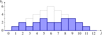
Figure 1: Example of a configuration of entanglement heights ($h_{j}=\log_{2}D_{j}$) satisfying the height difference constraint $|h_{j}-h_{j-1}|\leq 1,\forall j$ when $n=12$. The dashed line shows the configuration with maximum heights.

Let us now show that the maximum height resulting from the application of $n_{g}$ two-bit gates is bounded by $h_{\rm max}\leq\lfloor\sqrt{2\,n_{g}}\rfloor$. The application of a single two-bit gate on bits $j-1$ and $j$ changes the height $h_{j-1}\to\tilde{h}_{j-1}=\min(h_{j-2},h_{j})+1$. Because the relative heights of neighboring bonds cannot differ by more than 1 unit due to the hdc, the maximum amount that the height $\tilde{h}_{j-1}$ can increase with respect to $h_{j-1}$ is by 2 (which occurs when $h_{j-2}=h_{j}=h_{j-1}+1$). Therefore one can write that $S=\sum_{i}h_{i}\leq 2\,n_{g}$. Now, suppose that the maximum height is $h_{\rm max}$ at some bond labelled by $i_{\rm max}$ (located to the right of bit $i_{\rm max}$); because the heights $h_{0}$ to the left of the 1st bit and $h_{n}$ to the right of the $n$th bit are both equal to 0 at all times, and because of the hdc condition, there are constraints on how quickly the heights can grow from 0 to $h_{\rm max}$ at $i_{\rm max}$ and then decrease down to 0 again. The climb and descent that minimize the area $S$ can be trivially seen to be a triangle where $h_{j}$ increases linearly from $j=i_{\rm max}-h_{\rm max}$ to $j=i_{\rm max}$, and then decreases linearly until $j=i_{\rm max}+h_{\rm max}$. The area of this triangle is $S_{\rm min}=h_{\rm max}^{2}$, and any other height profile that reaches the same maximum height $h_{\rm max}$ has equal or larger area. Therefore, $h_{\rm max}^{2}\leq S\leq 2\,n_{g}$, and thus we arrive at the conclusion that $h_{\rm max}\leq\lfloor\sqrt{2\,n_{g}}\rfloor$, i.e., the bound on the maximum entanglement height for a given number of gates. Furthermore, because of the hdc and the fact that $h_{0}=h_{n}=0$, the entanglement height for a fixed $j$ is bounded by $h_{j}\leq\min(j,n-j)$, and the overall maximum $h_{\rm max}=\lfloor n/2\rfloor$ is reached at the center of the chain, $j=\lfloor n/2\rfloor$ and $j=\lceil n/2\rceil$ (which coincide when $n$ is even).

Putting all the conditions together, we arrive at $h_{\rm max}\leq\min\left(\lfloor\sqrt{2\,n_{g}}\rfloor,\lfloor n/2\rfloor\right)$, or equivalently, the bound $D\leq D_{\rm max}(n,n_{g})=\min\left(2^{\lfloor\sqrt{2n_{g}}\rfloor},2^{\lfloor n/2\rfloor}\right)$ which we used to obtain the absolute maximum running time of the search algorithm.

Conclusions – We have shown that it is possible to achieve virtual parallelization in single-processor classical computers using one-bit and two-bit local gates acting on matrix product states over $n$ bits. Based on this method, we propose a search algorithm that runs in subexponential time when the cost to check a witness requires less than $O(n^{2})$ two-bit gates. This critical bound in the circuit size was obtained assuming a worst-case scenario for the matrix dimension growth as a function of the number of two-bit gates. However, for particular circuits, the actual rank of the matrices may grow slower than this estimate, in which case some speedup is possible. In addition, during gate operations and matrix decompositions, if the singular values decay sufficiently fast, it may be possible to reduce matrix rank growth through truncation, similarly to the standard procedure used in quantum methods such as the TEBD vidal and its classical version for stochastic evolution, the cTEBD temme2010 ; johnson2010 . This question is open to future investigation.

The method is not limited to one-dimensional bit arrays and could, in principle, be extended to higher dimension tensor products. Finally, we point out that the method also naturally counts the number of satisfying assignments of a given Boolean formula, which is a problem of much importance in computer science.

This work was supported in part by the NSF grants CCF-1116590 and CCF-1117241. The authors thank P. Wocjan for useful discussions.

References

- (1) D. Deutsch, Proc. R. Soc. Lond. A 400, 97 (1985).
- (2) P. W. Shor, SIAM J. Sci. Stat. Comput. 26, 1484 (1997).
- (3) L. K. Grover, Phys. Rev. Lett. 79, 325 (1997).
- (4) G. Vidal, Phys. Rev. Lett. 91, 147902 (2003); G. Vidal, ibid 93, 040502 (2004).
- (5) F. Verstraete, V. Murg, and J. I. Cirac, Adv. Phys. 57, 143 (2008).
- (6) J. I. Cirac and F. Verstraete, J. Phys. A 42, 504004 (2009).
- (7) A. Hamma, S. Santra, and P. Zanardi, arXiv:1109.4391.
- (8) B. Derrida, M. R. Evans, H. Hakim, and V. Pasquier, J. Phys. A 26, 1493 (1993).
- (9) K. Temme and F. Verstraete, Phys. Rev. Lett. 104, 210502 (2010).
- (10) T. H. Johnson, S. R. Clark, and D. Jaksch, Phys. Rev. E 82, 036702 (2010).