Variance of Linear Statistic for Plancherel Young Diagrams

Abstract

In this paper we compute the precise asymptotics of the variance of linear statistic of descents on a growing interval for Plancherel Young diagrams (following Vershik and Kerov, diagrams are considered rotated by $\pi/4$). We also give an example of a local configuration with linearly growing variance in a fixed regime and prove the central limit theorem for this configuration in the given regime.

1 Introduction

Young diagram $\lambda$ with $n$ cells is a table, rows of which represent a partition of $n$ to the sum of nonincreasing summands $\lambda_{1}\geq\lambda_{2}\geq...\geq\lambda_{m}>0,\,\lambda_{1}+...+\lambda_{m}=n$. Set $n=|\lambda|$. We denote $\mathbb{Y}_{n}$ the set of Young diagrams with $n$ cells. Following Vershik and Kerov we will draw diagrams rotated by $\dfrac{\pi}{4}$:

For a diagram $\lambda$ define a sequence $(c_{i}(\lambda))\in\{0,1\}^{\mathbb{Z}}$ as follows:

$$\begin{cases}c_{k}(\lambda)=1,&k=\lambda_{i}-i,\text{for some }i;\\ c_{k}(\lambda)=0,&\text{otherwise}.\end{cases}$$

This sequence has the following geometrical interpretation. Consider a function $\Phi_{\lambda}$ whose graph represents the upper edge of a rotated diagram. The sequence $c_{i}(\lambda)$ is the sequence of descents of a rotated diagram, that is, $\Phi_{\lambda}$ is a continuous piecewise-linear function with the following property:

$$\begin{cases}\Phi_{\lambda}^{\prime}(x)=1,&c_{[x]}(\lambda)=0;\\ \Phi_{\lambda}^{\prime}(x)=-1,&\text{otherwise}.\end{cases}$$

The probability measure $\mathbb{P}l^{(n)}$ on $\mathbb{Y}_{n}$ is given by the formula

$$\mathbb{P}l^{(n)}(\lambda)=\frac{(\dim\lambda)^{2}}{n!},$$

where $\dim\lambda$ is the dimension of the irreducible representation of the symmetric group $\mathbb{S}_{n}$ corresponding to $\lambda$. This measure is called the Plancherel measure.

It is shown in [2] and [7] that the local distribution of $c_{i}(\lambda)$ as ${|\lambda|\to\infty}$ is governed by the discrete determinantal sine-process. For the reader’s convenience we recall the statement of Theorem 2 from [2]: for an arbitrary subset $\{d_{1},...,d_{s}\}\subset\mathbb{Z}$ and a sequence $(x_{n}),\lim\limits_{n\to\infty}x_{n}/\sqrt{n}=u\in(-2,2)$ the following holds:

$$\lim\limits_{n\to\infty}\mathbb{E}_{\mathbb{P}l^{(n)}}(c_{x_{n}+d_{1}}(\lambda)c_{x_{n}+d_{2}}(\lambda)...c_{x_{n}+d_{s}}(\lambda))=\det\left[K_{\sin}(d_{i}-d_{j},\arccos(u/2))\right]_{1\leq i,j\leq s},$$

where $K_{\sin}(x,\phi)$ is the sine kernel,

$$K_{\sin}(x,\phi)=\frac{\sin(\phi(x-y))}{\pi(x-y)}.$$

(for the more general statement see [2]).

In this paper we are concerned with the linear statistic $\displaystyle{\sum_{i\in I}c_{i}}$ of descents for Plancherel Young diagrams. The main result of this paper is the precise asymptotics for the variance of the linear statistic of $c_{i}$:

Theorem 1.

For all $a,b\in(-2,2)$ and all sequences ${x_{n}},{y_{n}}$ such that $\lim\limits_{n\to\infty}{\dfrac{x_{n}}{\sqrt{n}}=a}$, $\lim\limits_{n\to\infty}\dfrac{y_{n}}{\sqrt{n}}=b$ and $\lim\limits_{n\to\infty}(y_{n}-x_{n})=+\infty$, the following holds:

$$\lim\limits_{n\to\infty}\frac{Var_{\mathbb{P}l^{(n)}}\left(\displaystyle{\sum\limits_{i=x_{n}}^{y_{n}}}c_{i}(\lambda)\right)}{\log(y_{n}-x_{n})}=\frac{1}{\pi^{2}}.$$ (1)

Plan of the proof and organization of the paper

To prove Theorem 1 we use the theorem established, independently and simultaneously, by Borodin, Okounkov and Olshanski [2] and Johansson [7], which claims that the poissonization of the Plancherel measure is the discrete Bessel determinantal point process. In Section 3 we analyze the asymptotics of the poissonized variance in the left part of (1). In Section 4 switch to the asymptotics with respect to the Plancherel measure (depoissonization) is described. Estimates of the Bessel kernel that we need in Section 3 are proved in Section 5.

Using general properties of determinantal point processes it is easy to obtain an upper bound for the variance of frequency of general local patterns on Young diagram. In Section 6 we give an example of local patterns with linearly growing variance and prove the central limit theorem for them.

Acknowledgements

I am deeply grateful to Alexander Bufetov for the statement of the problem and for many helpful discussions. I am deeply grateful to Vadim Gorin, Sevak Mkrtchyan and Grigori Olshanski for helpful discussions.

2 Poissonization

To prove Theorem 1 we use the poissonization([2], [7]). Set $\mathbb{Y}=\bigcup\limits_{n=1}^{\infty}\mathbb{Y}_{n}$, and for $\eta\in\mathbb{C}$ let

$$\mathbb{P}l_{\eta}(\lambda)=e^{-\eta}\sum_{k=0}^{\infty}\frac{\eta^{k}}{k!}\mathbb{P}l^{(k)}(\lambda),\,\eta\in\mathbb{C},$$

be the poissonization of Plancherel measure (set $\mathbb{P}l^{(k)}(\lambda)=0$ when $|\lambda|\neq k$). Borodin, Okounkov, Olshanski in [2] and Johansson in [7] showed that $\mathbb{P}l_{\eta}$ induces the determinantal point process on the set of Young diagrams: denote $\eta=\theta^{2}$; for an arbitrary subset $\{x_{1},...,x_{s}\}\subset\mathbb{Z}$ the following holds:

$$\mathbb{E}_{\mathbb{P}l_{\theta^{2}}}(c_{x_{1}}(\lambda)c_{x_{2}}(\lambda)...c_{x_{s}}(\lambda))=\det\left[J(x_{i},x_{j},\theta^{2})\right]_{1\leq i,j\leq s},$$

where $J(x,y,\theta^{2})$ is the Bessel kernel defined by

$$J(x,y,\theta^{2})=\theta\frac{J_{x}(2\theta)J_{y+1}(2\theta)-J_{x+1}(2\theta)J_{y}(2\theta)}{x-y}.$$

(from now on we understand variance and expectation with respect to $\mathbb{P}l_{\theta^{2}}$ for $\theta\in\mathbb{C}$ formally).

It was shown in [2] and [7] that local patterns of a Young diagram are governed by the sine-process (i.e. the Bessel kernel degenerates to the sine kernel as $n\to\infty$).

There are continuous versions of sine and Bessel processes, see [14], [5], [13]. The central limit theorem for the continuous sine-process was proved in [5]. The central limit theorem for the continuous Bessel process was proved in [13]. Note that in both cases one has a logarithmic growth of the variance of the linear statistics. See [14] for the central limit theorem and other general results for determinantal point processes.

Following [4] and using the well-known identity

$$J(x,x,\theta^{2})=\sum\limits_{y\in\mathbb{Z}}\left(J(x,y,\theta^{2})\right)^{2},$$

which represents the fact that the linear operator defined by the kernel $J$ is a projection (see [2]), we rewrite the poissonized variance from 1 in the following way:

$$Var_{\theta^{2}}\left(\sum\limits_{x}^{y}c_{i}(\lambda)\right)=\sum\nolimits_{i\in[x_{n},y_{n}]}\sum\nolimits_{j\notin[x_{n},y_{n}]}\left(J(i,j,\theta^{2})\right)^{2},$$

where $Var_{\theta^{2}}$ is the variance with respect to the poissonization of the Plancherel measure $\mathbb{P}l_{\theta^{2}}$. Now we formulate the poissonized version of Theorem 1.

Proposition 2.1.

There is a constant $\gamma>0$ such that for all $a,b\in(-2,2)$ and all sequences ${x_{n}},{y_{n}}$ such that $\lim\limits_{n\to\infty}\dfrac{x_{n}}{\sqrt{n}}=a$, $\lim\limits_{n\to\infty}\dfrac{y_{n}}{\sqrt{n}}=b$ and ${\lim\limits_{n\to\infty}(y_{n}-x_{n})=\infty}$ the following holds:

$$\left|\frac{\displaystyle{\sum\nolimits_{i\in[x_{n},y_{n}]}\sum\nolimits_{j\notin[x_{n},y_{n}]}}\left(J(i,j,\theta^{2})\right)^{2}}{\log(y_{n}-x_{n})}-\frac{1}{\pi^{2}}\right|\exp(-\gamma|\sqrt{n}-\theta|)=o(1).$$ (2)

Similar proposition is stated in [1]. Note that Proposition 2 immediately yields an asymptotical formula for the variance of poissonized measure $Pl_{n},{n>0}$, and from the Soshnikov’s central limit theorem from [14] we get

Proposition 2.2.

For all $a,b\in(-2,2)$ and all sequences ${x_{n}},{y_{n}}$ such that ${\lim\limits_{n\to\infty}\dfrac{x_{n}}{\sqrt{n}}=a}$, ${\lim\limits_{n\to\infty}\dfrac{y_{n}}{\sqrt{n}}=b}$ and $\lim\limits_{n\to\infty}(y_{n}-x_{n})=+\infty$ the following holds:

$$\frac{\sum_{i\in[x_{n},y_{n}]}c_{i}(\lambda)-\mathbb{E}_{n}(\sum_{i\in[x_{n},y_{n}]}c_{i}(\lambda))}{\frac{1}{\pi}\sqrt{\log(y_{n}-x_{n})}}\xrightarrow[d]{}\mathcal{N}(0,1)$$

as $n\to\infty$.

Here $\xrightarrow[d]{}$ means convergence in distribution.

The central limit theorem for the integral of the deviation of a Young diagram from its limit shape is proved in [6], [8]. The central limit theorem for the point-wise deviation is stated in [1].

It is clear from the sine kernel asymptotics that expectation of linear statistic $\mathbb{E}\left(\sum c_{i}\right)$ grows linearly in ${(y_{n}-x_{n})}$.

One may come back to the Plancherel measure from its poissonization using the depoissonization lemma (Lemma 3.1 in [2]) and some of its modifications (Lemmas 3.1 - 3.2 in [4]).

Fix $0<\alpha<1/4$.

Depoissonization Lemma 1.

Let $\{f_{n}\}$ be a sequence of entire functions,

$$f_{n}=e^{-z}\sum_{k=0}^{\infty}\frac{f_{nk}}{k!}z^{k},$$

and assume that there exist constants $f_{\infty}$ and $\gamma$ such that

$$\max_{|z|=n}f_{n}(z)=O(e^{\gamma\sqrt{n}})$$

and

$$\max_{|z/n-1|\leq n^{-\alpha}}|f_{n}(z)-f_{\infty}|e^{-\gamma|z-n|/\sqrt{n}}=o(1)$$

as $n\rightarrow\infty$. Then

$$\lim_{n\rightarrow\infty}f_{nn}=f_{\infty}.$$

Depoissonization Lemma 2.

Let $\{f_{n}\}$ be a sequence of entire functions,

$$f_{n}=e^{-z}\sum_{k=0}^{\infty}\frac{f_{nk}}{k!}z^{k},$$

and assume that there exist constants $f_{\infty}$, $\gamma$, $C_{1}$, $C_{2}$ such that

$$\max_{|z|=n}|f_{n}(z)|\leq C_{1}e^{\gamma\sqrt{n}},$$

$$\max_{|z/n-1|\leq n^{-\alpha}}|f_{n}(z)-f_{\infty}|e^{-\gamma|z-n|/\sqrt{n}}\leq C_{2}.$$

Then there exists a constant $C=C(\gamma,C_{1},C_{2})$ such that for all ${n>0}$ we have

$$|f_{nn}-f_{\infty}|<C.$$

Depoissonization Lemma 3.

Assume that $\delta>0$ and there exist constants $f_{\infty},\gamma_{1},\gamma_{2},\gamma_{3},C_{1}$, $\tilde{C},C_{2},C_{3}>0,$ such that

$$\max_{|z|=n}|f_{n}(z)|\leq C_{1}(e^{\gamma_{1}\sqrt{n}}),$$

$$\max_{|z/n-1|<n^{-\alpha}}|f_{n}(z)|e^{-\frac{\gamma_{2}|z-n|}{\sqrt{n}}}\leq C_{2},$$

$$\max_{|z/n-1|<n^{\delta-1}}|f_{n}(z)-f_{\infty}|e^{-\frac{\gamma_{3}|z-n|}{\sqrt{n}}}\leq C_{3}.$$

Let $a_{n}$ be a sequence of positive numbers, $|a_{n}|<\tilde{C}$, and assume that

$$\max_{|z/n-1|<n^{\delta-1}}|f_{n}(z)-f_{\infty}|e^{\frac{-\gamma_{1}|z-n|}{\sqrt{n}}}\leq C_{1}a_{n}.$$

Then there exists a constant $C=C(\gamma_{1},\gamma_{2},\gamma_{3},C_{1},\tilde{C},C_{2},C_{3})$ such that for all ${n>0}$ we have

$$|f_{nn}-f_{\infty}|<Ca_{n}.$$

3 Asymptotics of the poissonized variance

3.1 Estimates of the Bessel kernel

To prove Proposition 2.1 we need the following estimates of the discrete Bessel kernel (we postpone the proof to the last Section). Set

$$u_{x}=x/\sqrt{n},u_{y}=y/\sqrt{n},\phi_{x}=\arccos(u_{x}/2),\phi_{y}=\arccos(u_{y}/2).$$

Proposition 3.1 (points are far from the edge of the spectrum).

Let

$$|x|<2\sqrt{n}-n^{\delta_{1}},\,|y|<2\sqrt{n}-n^{\delta_{2}},\,\delta_{1},\delta_{2}>1/6.$$

Then

$$|J(x,y,\theta^{2})|\leq\frac{C\exp(\gamma|\theta-\sqrt{n}|)}{|e^{i\phi_{x}}-e^{i\phi_{y}}|\sqrt[4]{2-u_{x}}\sqrt[4]{2-u_{y}}\sqrt{n}}+$$

$$+\exp\left(-n^{c(-1/6+\max(\delta_{1},\delta_{2}))}+\gamma|\theta-\sqrt{n}|\right).$$

Proposition 3.2 (one of the points is at the edge of the spectrum).

Let

$$|x|<2\sqrt{n}-n^{\delta},2\sqrt{n}-n^{1/6}<|y|<2\sqrt{n}+n^{1/6},\delta>1/6.$$

Then

$$|J(x,y,\theta^{2})|\leq\left(\frac{C}{n^{5/12}\left(2-u_{x}\right)^{3/4}}+O(e^{-n^{c(\delta-1/6)}})\right)\exp(\gamma|\theta-\sqrt{n}|).$$

Proposition 3.3 (one of the points is beyond the edge of the spectrum).

Let

$$|x|<2\sqrt{n},|y|>2\sqrt{n}+n^{\delta},\delta>1/6.$$

Then

$$|J(x,y,\theta^{2})|\leq\left(Ce^{-n^{c(\delta-1/6)}}\right)\exp(\gamma|\theta-\sqrt{n}|).$$

3.2 Proof of Proposition 2.1

We now rewrite the estimate from Proposition 3.1.

$$\frac{C}{|e^{i\phi_{x}}-e^{i\phi_{y}}|\sqrt[4]{2-u_{x}}\sqrt[4]{2-u_{y}}\sqrt{n}}\leq\frac{C}{|\sqrt{2-u_{x}}-\sqrt{2-u_{y}}|\sqrt[4]{2-u_{x}}\sqrt[4]{2-u_{y}}\sqrt{n}},$$

Using the equality

$$(a^{2}-b^{2})ab=(a^{4}-b^{4})\frac{ab}{a^{2}+b^{2}},$$

we get

$$J(x,y,\theta^{2})\leq\frac{C\exp{\gamma|\theta-\sqrt{n}|}}{|x-y|}\left(\frac{\sqrt[4]{2-u_{x}}}{\sqrt[4]{2-u_{y}}}+\frac{\sqrt[4]{2-u_{y}}}{\sqrt[4]{2-u_{x}}}\right).$$

Divide the interval of summation into three parts:

$$R_{1}=\{(i,\,j)\in\mathbb{Z}^{2}|\,i\in(x+\delta,\,y-\delta),\,j\notin[x,\,y]\}$$

$$R_{2}=\{(i,\,j)\in\mathbb{Z}^{2}|\,(i\in[x,\,x+\delta],\,j\notin[i-\delta-1,\,x-1]\cup[x,y])\vee$$

$$\vee(i\in[y-\delta,\,y],\,j\notin[y+1,\,i+\delta+1]\cup[x,y])\}$$

$$M=\{(i,\,j)\in\mathbb{Z}^{2}|\,(i\in[x,\,x+\delta],\,j\in[i-\delta-1,\,x-1])\vee$$

$$\vee(i\in[y-\delta,\,y],\,j\in[y+1,\,i+\delta+1])\}$$

where $\delta=\varepsilon(x-y)$ will be chosen later. Following [3] we are going to estimate the sum from parts $R_{1}$ and $R_{2}$, which may be neglected, and compute it in M.

Estimate in $R_{1}$:

Write down the sum from $R_{1}$:

$$\sum_{i\in(x+\delta,y-\delta)}\sum_{j\notin[x,y]}J^{2}(i,j,\theta^{2})=\sum_{i\in(x+\delta,y-\delta)}\sum_{j=-\infty}^{x-1}J^{2}(i,j,\theta^{2})+\\ +\sum_{i\in(x+\delta,y-\delta)}\sum_{j=y+1}^{\infty}J^{2}(i,j,\theta^{2}).$$ (3)

We estimate the first summand (the second one may be estimated similarly)

Summing in $j$ we have:

$$\sum_{j=y+1}^{\infty}J^{2}(i,j,\theta^{2})=\sum_{j=y+1}^{2\sqrt{n}-n^{1/6}}J^{2}(i,j,\theta^{2})+\\ +\sum_{j=2\sqrt{n}-n^{1/6}}^{2\sqrt{n}+n^{1/6}}J^{2}(i,j,\theta^{2})+\sum_{j=2\sqrt{n}+n^{1/6}}^{\infty}J^{2}(i,j,\theta^{2}).$$ (4)

We estimate the first summand from (4):

$$\exp(-\gamma|\theta-\sqrt{n}|)\sum_{j=y+1}^{2\sqrt{n}-n^{1/6}}J^{2}(i,j,\theta^{2})\leq\\ \leq\sum_{j=y+1}^{2\sqrt{n}-n^{1/6}}\frac{C}{(j-i)^{2}}\left(\frac{\sqrt[4]{2-u_{i}}}{\sqrt[4]{2-u_{j}}}+\frac{\sqrt[4]{2-u_{j}}}{\sqrt[4]{2-u_{i}}}\right)^{2}\leq\\ \leq\sum_{j=y+1}^{2\sqrt{n}-n^{1/6}}\frac{C}{(j-i)^{2}}\left(\frac{\sqrt{2-u_{i}}}{\sqrt{2-u_{j}}}+\frac{\sqrt{2-u_{j}}}{\sqrt{2-u_{i}}}\right)\leq\\$$ (5)

$$\leq C\intop_{y+1}^{2\sqrt{n}-n^{1/6}}\frac{1}{(t-i)^{2}}\left(\frac{\sqrt{2\sqrt{n}-i}}{\sqrt{2\sqrt{n}-t}}+\frac{\sqrt{2\sqrt{n}-t}}{\sqrt{2\sqrt{n}-i}}\right)dt=\\ =-C\frac{1}{t-i}\frac{\sqrt{2\sqrt{n}-t}}{\sqrt{2\sqrt{n}-i}}\bigg{|}_{y+1}^{2\sqrt{n}-n^{1/6}}=\\ =-C\left(\frac{n^{1/6}}{(2\sqrt{n}-i-n^{1/6})\sqrt{2\sqrt{n}-i}}-\frac{\sqrt{2\sqrt{n}-y-1}}{(y+1-i)\sqrt{2\sqrt{n}-i}}\right)\leq\\ \leq\frac{C}{y-i+1}.$$ (6)

Now sum in $i$:

$$\sum_{i\in(x+\delta,y-\delta)}\frac{C}{y-i+1}\leq C\ln(\frac{y-x}{\delta}).$$

Now estimate the second summand:

$$\sum_{j=2\sqrt{n}-n^{1/6}}^{2\sqrt{n}+n^{1/6}}J^{2}(i,j,\theta^{2})\leq\sum_{j=2\sqrt{n}-n^{1/6}}^{2\sqrt{n}+n^{1/6}}\frac{C\exp(\gamma|\theta-\sqrt{n}|)}{n^{5/6}\left(2-u_{i}\right)^{3/2}}=C\frac{\exp(\gamma|\theta-\sqrt{n}|)n^{1/12}}{(2\sqrt{n}-i)^{3/2}}.$$

Sum this estimate in $i$:

$$\sum_{i\in(x+\delta,y-\delta]}\frac{n^{1/12}}{(2\sqrt{n}-i)^{3/2}}\leq Cn^{1/12}\intop_{x}^{y}\frac{1}{(2\sqrt{n}-t)^{3/2}}dt=\\ =Cn^{1/12}\left(\frac{1}{\sqrt{2\sqrt{n}-t}}\right)\bigg{|}_{x}^{y}\leq\frac{Cn^{1/12}}{\sqrt{2\sqrt{n}-y}}\leq\\ \leq Cn^{1/12-1/4}=o(1).$$ (7)

The third summand is exponentially small by Proposition 3.3.

Estimate in $R_{2}$:

$$\sum_{i\in[y-\delta,\,y]}\sum_{j\notin[y+1,\,i+\delta+1]}J^{2}(x,y,\theta^{2})\leq\sum_{i\in[y-\delta,\,y]}\frac{\exp(\gamma|\theta-\sqrt{n}|)}{\delta}=O(1)\exp(\gamma|\theta-\sqrt{n}|).$$

Asymptotics in $M$:

From the Debye asymptotics for the Bessel function we get:

$$J(x,y,\theta^{2})=\frac{\sin(\phi_{y}(x-y))}{\pi(x-y)}+o(\exp(\gamma|\theta-\sqrt{n}|)),$$ (8)

(see the proof of Lemma 3.5 in [2]) which implies

$$\sum_{i\in[y-\delta,\,y]}\sum_{j\in[y+1,\,i+\delta+1]}J^{2}(x,y,\theta^{2})=\\ =\sum_{i\in[y-\delta,\,y]}\sum_{j\in[y+1,\,i+\delta+1]}\frac{1}{\pi^{2}}\frac{\sin^{2}(\phi_{y}(i-j))}{(i-j)^{2}}(1+o(1))+o(e^{\gamma|n-\theta^{2}|/\sqrt{n}}),$$ (9)

In sums of this kind replacement of $\sin^{2}(\cdot)$ by its mean value $\frac{1}{2}$ does not change the asymptotics. More precisely, we now use Lemma 4.6 from [3] on our kernel making the change in parameters as follows:

$$i=\xi_{1}+y-\delta,\,j=\xi_{2}+y+1.$$

We obtain

$$\sum_{i\in[y-\delta,\,y]}\sum_{j\in[y+1,\,i+\delta+1]}\frac{1}{\pi^{2}}\frac{\sin^{2}(\phi(i-j))}{(i-j)^{2}}=\\ =\sum_{i\in[y-\delta,\,y]}\sum_{j\in[y+1,\,i+\delta+1]}\frac{1}{2\pi^{2}}\frac{1}{(i-j)^{2}}(1+o(1))=\\ =\frac{1}{2\pi^{2}}\ln\delta(1+o(1)).$$ (10)

Now set $\delta=\dfrac{|x-y|}{\ln(|x-y|)}$. This choice of $\delta$ implies that the sum in $R_{1}\leq C\ln\ln(x-y)$, and that finishes the proof of Proposition 2.1.

4 Depoissonization

In this section we finish the proof of Theorem 1. Note that the depoissonization techniques described above may be applied only to quantities linear in measure (i.e. to an expectation, not variance). That is why we will now, following [4], find an expectation with the same asymptotics as our poissonized and original variances has. To do this we will need Lemma 6.3 from [4] and its depoissonization:

Proposition 4.1.

There exists $\varepsilon_{0}>0$ such that the following holds. For all $\delta_{0}>\dfrac{1}{6}$ there exist constants $C>0$, $\gamma>0$ such that for all $n\in\mathbb{N}$, all $x,|x|<2\sqrt{n}-n^{\delta_{0}}$ and all $\theta\in\mathbb{C}$ such that

$$\left|\frac{\theta}{\sqrt{n}}-1\right|<\varepsilon_{0}$$

we have

$$|J(x,x,\theta^{2})-\frac{1}{\pi}\arccos\frac{x}{2\sqrt{n}}|\leq\frac{\exp(\gamma|\theta-\sqrt{n}|)}{2\sqrt{n}-x}.$$

Proposition 4.2.

For all $\delta_{0}>\frac{1}{6}$ there exists a constant $C$ such that

$$|\mathbb{E}_{\mathbb{P}l^{(n)}}(c_{x})-\frac{1}{\pi}\arccos\frac{x}{2\sqrt{n}}|\leq\frac{C(2-|u_{x}|)}{\sqrt{n}},$$

for all $x,|x|<2\sqrt{n}-n^{\delta_{0}}$.

Write

$$Var_{\theta^{2}}\left(\sum_{i=k}^{k+l}c_{i}\right)=\mathbb{E}_{\theta^{2}}\left(\sum_{i=k}^{k+l}c_{i}-\sum_{i=k}^{k+l}\mathbb{E}_{\theta^{2}}c_{i}\right)^{2}=\\ =\mathbb{E}_{\theta^{2}}\left(\sum_{i=k}^{k+l}c_{i}-\sum_{i=k}^{k+l}J(i,i,\theta^{2})\right)^{2}.$$ (11)

Set

$$\Omega(t)=\begin{cases}\frac{2}{\pi}(t\arcsin(t/2)+\sqrt{4-t^{2}}),&\text{if $|t|\leq 2$;}\\ |t|,&\text{if $|t|>2$, }\end{cases}$$

$$F_{\lambda}(t)=\Phi_{\lambda}(t)-\sqrt{n}\Omega(t/\sqrt{n}),$$

where $\Phi_{\lambda}(t)$ is a function representing the upper edge of the diagram $\lambda$. Note that $\Omega(t)$ is the limit shape of Plancherel Young diagrams (see [9], [11] for details). Now write

$$F_{\lambda}(k+1)-F_{\lambda}(k)=1-2c_{k}(\lambda)-\sqrt{n}\left(\Omega\left(\frac{k+1}{\sqrt{n}}\right)-\Omega\left(\frac{k}{\sqrt{n}}\right)\right)=\\ =2\left(\frac{\arccos\frac{k}{2\sqrt{n}}}{\pi}-c_{k}(\lambda)\right)+\frac{2}{\pi}\arcsin\left(\frac{k}{2\sqrt{n}}\right)-\sqrt{n}\left(\Omega\left(\frac{k+1}{\sqrt{n}}\right)-\Omega\left(\frac{k}{\sqrt{n}}\right)\right)=\\ =2\left(J(k,k;\,\theta^{2})-c_{k}(\lambda)\right)+2\left(\frac{\arccos\frac{k}{2\sqrt{n}}}{\pi}-J(k,k;\,\theta^{2})\right)+\\ +\left(\,\frac{2}{\pi}\arcsin\left(\frac{k}{2\sqrt{n}}\right)-\sqrt{n}\left(\Omega\left(\frac{k+1}{\sqrt{n}}\right)-\Omega\left(\frac{k}{\sqrt{n}}\right)\right)\right).$$

From the Taylor formula for $\Omega$ we have

$$\left|\sqrt{n}\left(\Omega\left(\frac{k+1}{\sqrt{n}}\right)-\Omega\left(\frac{k}{\sqrt{n}}\right)\right)-\frac{2}{\pi}\arcsin\left(\frac{k}{2\sqrt{n}}\right)\right|\leq\frac{10}{\sqrt{4n-k^{2}}}.$$

Summing these estimates and applying Proposition 4.1 we obtain that after the depoissonization

$$\lim_{n\rightarrow\infty}\frac{\mathbb{E}_{\mathbb{P}l^{(n)}}\left(F_{\lambda}(k+l)-F_{\lambda}(k)\right)^{2}}{\log l}=\frac{1}{\pi^{2}}.$$

In the same way, applying Proposition 4.2, we finish the proof of Theorem 1.

5 Proofs of the estimates of the Bessel kernel

Plan of the proofs

We are using the Okounkov’s integral representation of the kernel ([12]):

$$J(x,y,\theta^{2})=\frac{1}{(2\pi i)^{2}}\intop\intop_{|z|<|w|}\frac{\exp(\theta\left(z-\frac{1}{z}-w+\frac{1}{w}\right))}{(z-w)z^{x+1}w^{-y}}dzdw.$$

Set

$$u_{x}=\frac{x}{\sqrt{n}},\,S(z,u)=z-\frac{1}{z}-u\ln z,\,\phi_{x}=\arccos\frac{u_{x}}{2}.$$

Denote

$$\Phi(z,w,\theta)=\frac{\exp\theta\left(z-\frac{1}{z}-w+\frac{1}{w}\right)}{(z-w)z^{x+1}w^{-y}}.$$

Now note that

$$|\Phi(z,w,\theta)|\leq\exp(\gamma|\theta-\sqrt{n}|)|\Phi(z,w,\sqrt{n})|=\exp(\gamma|\theta-\sqrt{n}|)\left|\frac{\exp\sqrt{n}(S(z,u_{x})-S(z,u_{y}))}{z(z-w)}\right|.$$

This allows us to work with the Bessel kernel of a real parameter,

The proof is carried out using the steepest descent method. Following [12] we deform initial contours so that they pass through critical points of $S(z,u)$ and then we estimate the absolute value of the integral splitting contours in parts.

5.1 Proof of Proposition 3.1

Without a loss of generality assume that $x>y.$ Set $I_{x}=[-n^{-\beta_{x}},n^{-\beta_{x}}],I_{y}=[-n^{-\beta_{y}},n^{-\beta_{y}}]$, $\beta_{x}$ and $\beta_{y}$ will be defined later.

We now deform the contours in the following way. Each one consists of four parts: two circular arcs and two intervals transversal to the unit circle, similarly to [4] (see Fig. 1).

Introduce the parametrization on the intervals:

$$I_{x}^{+}(t)=e^{i\phi_{x}}+At,\,I_{x}^{-}(t)=e^{-i\phi_{x}}+At,$$

$$I_{y}^{+}(t)=e^{i\phi_{y}}+Bs,\,I_{y}^{-}(t)=e^{-i\phi_{y}}+Bs,$$

$$t\in I_{x},s\in I_{y}.$$

Here $A,B\in\mathbb{C}$ are independent on $n$ and chosen such that the intervals are transversal to the unit circle.

Let $C_{x}^{\pm},C_{y}^{\pm}$ be the circular arcs of the contours (- for the inner part and + for the outer), 0 be the center of both circles and $1\pm cn^{-\beta_{x}}$, $1\pm cn^{-\beta_{y}}$ be their radii.

Figure 1: deformed contours.

Write

$$S(z(t),u)=e^{i\phi_{x}}+At-\frac{1}{e^{i\phi_{x}}+At}-u_{x}\ln\left(e^{i\phi_{x}}+At\right),$$

on the interval.

$$\frac{dS}{dt}\bigg{|}_{t=0}=\left(A+\frac{A}{\left(e^{i\phi_{x}}+At\right)^{2}}-\frac{u_{x}A}{e^{i\phi_{x}}+At}\right)\bigg{|}_{t=0}=0,$$

$$\frac{d^{2}S}{dt^{2}}\bigg{|}_{t=0}=\left(-\frac{2A^{2}}{\left(e^{i\phi_{x}}+At\right)^{3}}+\frac{u_{x}A^{2}}{\left(e^{i\phi_{x}}+At\right)^{2}}\right)\bigg{|}_{t=0}=A^{2}(u_{x}e^{i\phi_{x}}-2)e^{-3i\phi_{x}}=\\ =A^{2}e^{-3i\phi_{x}}(u_{x}\cos\phi_{x}+iu_{x}\sin\phi_{x}-2)=2A^{2}e^{-3i\phi_{x}}\sin\phi_{x}(i\cos\phi_{x}-\sin\phi_{x})=\\ =2iA^{2}e^{-2i\phi_{x}}\sin\phi_{x}.$$ (12)

We used the fact that $u_{x}=2\cos\phi_{x}$. We obtain

$$\left|\Re\frac{d^{2}S}{dt^{2}}\bigg{|}_{t=0}\right|\geq C\sqrt{2-u}.$$

Recall that $f=\Theta(g)\iff f=O(g)\text{ and }g=O(f)$.

$$\frac{d^{3}S}{dt^{3}}\bigg{|}_{t=0}=\left(\frac{6A^{3}}{\left(e^{i\phi_{x}}+At\right)^{4}}-\frac{2u_{x}A^{3}}{\left(e^{i\phi_{x}}+At\right)^{3}}\right)|_{t=0}=6A^{3}e^{-4i\phi_{x}}-2u_{x}A^{3}e^{-3i\phi_{x}}=\\ =2A^{3}e^{-4i\phi_{x}}(3-u_{x}e^{i\phi_{x}})=\Theta(1).$$ (13)

$$\frac{d^{4}S}{dt^{4}}\bigg{|}_{t=0}=\left(-\frac{24A^{4}}{\left(e^{i\phi_{x}}+At\right)^{5}}+\frac{6u_{x}A^{4}}{\left(e^{i\phi_{x}}+At\right)^{4}}\right)|_{t=0}=24A^{4}e^{-5i\phi_{x}}-6u_{x}A^{4}e^{-4i\phi_{x}}=\\ =6A^{4}e^{-5i\phi_{x}}(-4+u_{x}e^{i\phi_{x}})=\Theta(1).$$ (14)

Derivatives $I_{y}^{\pm}(s)$ are estimated similarly.

Circular parts.

Switch to polar coordinates $z=(1+t)e^{i\phi}$.

$$\Re S(z,u)=(1+t-1+t-t^{2})\cos\phi(t)-u(t-t^{2}/2)+O(t^{3})=\\ =(2\cos\phi(t)-u)(t-t^{2}/2)+O(t^{3})=(2\cos(\arccos\frac{u}{2}+c_{1}t)-u)(t-t^{2}/2)+O(t^{3})=\\ =2ct(-\sin\arccos\frac{u}{2})t+O(t^{3})=-2c\sqrt{1-\frac{u^{2}}{4}}t^{2}+O(t^{3})=\\ =-c\sqrt{2-u}\sqrt{2+u}t^{2}+O(t^{3}),$$ (15)

$$\sqrt{n}\Re S(z,u)\leq-c\sqrt{n}\sqrt{2-u}t^{2}+\sqrt{n}O(t^{3}).$$

We want to deform the contours so that their intersection points are far enough from the unit circle, where $\Phi(z,w,\theta)$ is exponentially small. To guarantee that, we need the following conditions. Set $t=n^{-\beta}$ on both ends of the interval and write

1) $\sqrt{n(2-u)}t^{2}\to\infty$ as $n\to\infty$,

2) $\dfrac{t^{3}}{\sqrt{2-u}t^{2}}\to 0$ as $n\to\infty$,

3) $n^{-\beta}\leq c|e^{i\phi_{x}}-e^{i\phi_{y}}|$

Now we verify these conditions. $\sqrt{2-u}\geq n^{\delta/2-1/4},$ so 1) gives

$$\delta/2+1/4-2\beta>0\implies\beta<\delta/4+1/8,$$

and 2) gives

$$\delta/2-1/4>-\beta\implies\beta>1/4-\delta/2.$$

$\beta$ we need exists if

$$\delta/4+1/8>1/4-\delta/2\implies 3\delta/4>1/8,\,\delta>\frac{1}{6}.$$

Now consider 3). Let

$$x=2\sqrt{n}-n^{\delta}+an^{\alpha},\,y=2\sqrt{n}-n^{\delta}+bn^{\alpha},\,\delta>1/6,\,\alpha<\delta.$$

Then

$$|e^{i\phi_{x}}-e^{i\phi_{y}}|=\Theta(|\sin\phi_{x}-\sin\phi_{y}|)=\Theta(|\sqrt{2-u_{x}}-\sqrt{2-u_{y}}|),$$

$$\sqrt{n^{\delta-1/2}+an^{\alpha-1/2}}-\sqrt{n^{\delta-1/2}+bn^{\alpha-1/2}}=n^{\delta/2-1/4}\left(\sqrt{1+an^{\alpha-\delta}}-\sqrt{1+bn^{\alpha-\delta}}\right)=$$

$$=\Theta(n^{\alpha-1/4-\delta/2}).$$

as $n\to\infty$, and in this case there exists $C>0$ such that the following inequality holds:

$$\frac{C}{|e^{i\phi_{x}}-e^{i\phi_{y}}|\sqrt[4]{2-u_{x}}\sqrt[4]{2-u_{y}}\sqrt{n}}\geq\frac{C}{(a-b)n^{\alpha}}.$$

Rewrite 3) as follows:

$$n^{-\delta/4-1/8}<n^{-\beta}<n^{\alpha-1/4-\delta/2},$$

$$-\delta/4-1/8<\alpha-1/4-\delta/2,$$

$$\alpha>1/8+\delta/4.$$

It remains to consider

$$\alpha<1/8+\delta/4.$$

Note that in this case

$$\alpha-1/4-\delta/2<-\alpha.$$

We now estimate the integral in a neighborhood of the intersection along the intervals $J_{1},J_{2}$ of length

$$n^{\alpha-1/4-\delta/2}$$

(the intervals $AB$ and $CD$ on Fig. 2).

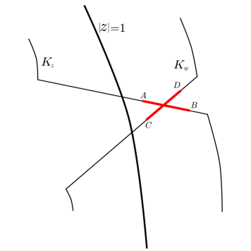
Figure 2: The integral along $AB$ and $CD$ gives the main contribution to the estimate.

$$\left|\intop_{J_{1}}\intop_{J_{2}}\Phi(z,w,\theta)dzdw\right|\leq\intop_{J_{1}}\intop_{J_{2}}|\Phi(z,w,\theta)|dzdw\leq\\ \leq\exp(\gamma|\theta-\sqrt{n}|)\intop_{J_{1}}\intop_{J_{2}}|\Phi(z,w,\sqrt{n})|dzdw\leq\exp(\gamma|\theta-\sqrt{n}|)\intop_{J_{1}}\intop_{J_{2}}\left|\frac{1}{\sqrt{c_{1}s^{2}+c_{2}t^{2}}}\right|dsdt\leq\\ \leq\exp(\gamma|\theta-\sqrt{n}|)C\max(|J_{1}|,|J_{2}|)\leq Cn^{-\alpha}.$$ (16)

Main contribution.

$$\left|\intop_{I_{x}^{+}}\intop_{I_{y}^{+}}\Phi(x,y,\theta)dzdw\right|\leq\exp(\gamma|\theta-\sqrt{n}|)\intop_{I_{x}}\intop_{I_{y}}\left|\frac{\exp(\sqrt{n}\left(S\left(z(t),u_{x}\right)-S(w(t),u_{y}\right)))}{e^{i\phi_{x}}-e^{i\phi_{y}}+At-Bs}\right|dsdt\leq\\ \leq\exp(\gamma|\theta-\sqrt{n}|)\frac{\intop_{I_{x}}\intop_{I_{y}}|\exp(\sqrt{n}\left(S\left(z(t),u_{x}\right)-S\left(w(t),u_{y}\right)\right))|dsdt}{|e^{i\phi_{x}}-e^{i\phi_{y}}|}=\\ =\exp(\gamma|\theta-\sqrt{n}|)\frac{\intop_{I_{x}}\intop_{I_{y}}|\exp\sqrt{n}\left(S_{x}^{\prime\prime}(0)t^{2}-S_{y}^{\prime\prime}(0)s^{2}+S_{x}^{(3)}(0)t^{3}-S_{y}{}^{(3)}(0)s^{3}+o(s^{3},t^{3})\right)|dsdt}{|e^{i\phi_{x}}-e^{i\phi_{y}}|}.$$ (17)

Write

$$s=\frac{s^{\prime}}{\sqrt[4]{n}\sqrt{|S_{y}^{\prime\prime}(0)|}},t=\frac{t^{\prime}}{\sqrt[4]{n}\sqrt{|S_{x}^{\prime\prime}(0)|}}.$$

Note that one can choose $\beta$ so that after change of variables the coefficient in the third term of the Taylor expansion goes to 0 as $n\to\infty$. Indeed, length of the new intervals of integration is equal to

$$n^{-\beta+1/4}\sqrt[4]{2-u}$$

and

$$\frac{\sqrt{n}t^{{}^{\prime}3}}{n^{3/4}\left(\sqrt{|S_{x}^{\prime\prime}|}\right)^{3}}\leq Cn^{-1/4}n^{3/8-3\delta/4}n^{-3\beta+3/4+3\delta/4-3/8}=Cn^{1/2-3\beta}\leq\\ \leq Cn^{1/2-3(1/8+\delta/4-\varepsilon)}=Cn^{1/8-3\delta/4+3\varepsilon}.\\$$ (18)

We get

$$\left|\intop_{I_{x}^{+}}\intop_{I_{y}^{+}}\Phi(x,y,\theta)dzdw\right|\leq C\exp(\gamma|\theta-\sqrt{n}|)\frac{|e^{i\phi_{x}}-e^{i\phi_{y}}|^{-1}}{\sqrt{n}\sqrt{S_{x}^{\prime\prime}}\sqrt{S_{y}^{\prime\prime}}}\leq\\ \leq C\exp(\gamma|\theta-\sqrt{n}|)\frac{|e^{i\phi_{x}}-e^{i\phi_{y}}|^{-1}}{\sqrt{n}\sqrt[4]{2-u_{x}}\sqrt[4]{2-u_{y}}}.$$ (19)

Same computations give the estimates of $|\intop_{I_{x}^{-}}\intop_{I_{y}^{-}}\Phi(x,y,\theta)dzdw|,\,|\intop_{I_{x}^{+}}\intop_{I_{y}^{-}}\Phi(x,y,\theta)dzdw|,$ $|\intop_{I_{x}^{-}}\intop_{I_{y}^{+}}\Phi(x,y,\theta)dzdw|$ and the estimate of the integral along the linear intervals in the case $\alpha\leq 1/8+\delta/4$.

Residue.

As we deform the contours we pick up the residue at $z=w$:

$$|Res|=\left|\dfrac{1}{2\pi i}\int_{re^{-i\phi}}^{re^{i\phi}}\dfrac{1}{w^{x-y+1}}dw\right|=\left|\dfrac{1}{2\pi ir^{x-y}}{\displaystyle\int_{e^{-i\phi}}^{e^{i\phi}}\dfrac{1}{t^{x-y+1}}dt}\right|=\left|\dfrac{1}{2\pi ir^{x-y}}K_{\sin}(x-y,\phi)\right|.$$

Note that $sgn(x-y)=sgn(r-1).$

5.2 Proof of Proposition 3.2

We deform the contours similarly to the case of Proposition 3.1, with $\beta_{y}=1/6$. In the case $y>2\sqrt{n}$ let contour $K_{w}$ be a circle with center in 0 and of radius $1+n^{-\beta_{y}}$. Consider parts of contours of length at most

$$\sqrt{|2-u_{y}|}<n^{-1/6}.$$

adjacent to $I_{x}^{\pm}$ and $I_{y}^{\pm}$ (for $y>2\sqrt{n}$ consider a circular part in the neighborhood of real axis) ($AB,CD,EF$ and $FG$ of Fig. 3).

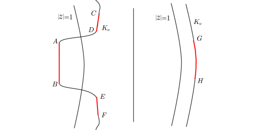
Figure 3: deformation of the contours for $y<2\sqrt{n}$ and $y>2\sqrt{n}$ respectively.

Write

$$\Re S(z,u)=(2\cos\phi(t)-u)(t-t^{2}/2)+O(t^{3}).$$

On these parts $\exp(n^{1/2}\Re S(z,u))=O(1)$ and beyond them on circular parts $n^{1/2}\Re S(z,u)$ is large: while $|2\cos\phi(t)-u|>\sqrt{|2-u_{y}|}$ we have

$$n^{1/2}\Re S(z,u)<-n^{1/6}.$$

Now estimate the contribution from integration along the intervals $I_{x}^{\pm}$ and $I_{y}^{\pm}$ similarly to (17) making another change of variables:

$$s=\frac{s^{\prime}}{n^{1/6}},t=\frac{t^{\prime}}{\sqrt[4]{n}\sqrt{|S_{x}^{\prime\prime}|}},$$

and

$$|z-w|>C|\sqrt{2-u_{x}}|.$$

The residue and contribution from the circular parts are estimated similarly to the proof of Proposition 3.1.

5.3 Proof of Proposition 3.3

In this case one may not deform the contours choosing their radii so that $\Phi(z,w,\theta)$ is exponentially small, see the estimate of the contribution from the circular parts in Proposition 3.1.

6 General local patterns

6.1 Variance for general local patterns

Denote $\vec{x}=\{x_{1},...,x_{k}\}\subset\mathbb{Z}$. Denote $c_{i+\vec{x}}=c_{i+x_{1}}c_{i+x_{2}}\cdots c_{i+x_{k}}$.

Proposition 6.1.

Let $\vec{x}\subset\mathbb{Z}$ be a finite set, $a,b\in(-2,2)$, and ${x_{n}},{y_{n}}$ be an integer sequence such that

$$\lim\limits_{n\to\infty}x_{n}/\sqrt{n}=a,\lim\limits_{n\to\infty}y_{n}/\sqrt{n}=b,y_{n}>x_{n}$$

and $\lim\limits_{n\to\infty}(y_{n}-x_{n})=+\infty$. Then there exists a constant $C>0$ such that

$$Var_{\mathbb{P}l^{(n)}}\left(\sum_{i=x_{n}}^{y_{n}}c_{i+\vec{x}}\right)\leq C(y_{n}-x_{n}).$$

We start with the proof of the poissonized version of this proposition:

$$Var_{\theta^{2}}\left(\sum_{i=x_{n}}^{y_{n}}c_{i+\vec{x}}\right)\leq(y_{n}-x_{n})C\exp(\gamma|\theta-\sqrt{n}|).$$ (20)

Rewrite our variance in the following way:

$$Var_{\theta^{2}}\left(\sum_{i=x_{n}}^{y_{n}}c_{i+\vec{x}}\right)=\mathbb{E}_{\theta^{2}}\left(\sum_{i}c_{i+\vec{x}}\right)+\mathbb{E}_{\theta^{2}}\left(\sum_{i\neq j}c_{i+\vec{x}}c_{j+\vec{x}}\right)-\\ -\sum_{i}\left(\mathbb{E}_{\theta^{2}}c_{i+\vec{x}}\right)^{2}-\sum_{i\neq j}\mathbb{E}_{\theta^{2}}c_{i+\vec{x}}\mathbb{E}_{\theta^{2}}c_{j+\vec{x}}.$$ (21)

Estimate the sum on the right hand side of (21):

$$\mathbb{E}_{\theta^{2}}\left(\sum_{i}c_{i+\vec{x}}\right)-\sum_{i}\left(\mathbb{E}_{\theta^{2}}c_{i+\vec{x}}\right)^{2}\leq C_{1}(y_{n}-x_{n})\exp(\gamma|\theta-\sqrt{n}|);$$

$$\left|\sum_{i,j:i+\vec{x}\cap j+\vec{x}\neq\varnothing}\mathbb{E}_{\theta^{2}}\left(\sum_{i\neq j}c_{i+\vec{x}}c_{j+\vec{x}}\right)-\sum_{i,j:i+\vec{x}\cap j+\vec{x}\neq\varnothing}\mathbb{E}_{\theta^{2}}c_{i+\vec{x}}\mathbb{E}_{\theta^{2}}c_{j+\vec{x}}\right|\leq C_{2}(y_{n}-x_{n})\exp(\gamma|\theta-\sqrt{n}|).$$

Note that if $i+\vec{x}\cap j+\vec{x}=\varnothing$, then

$$\mathbb{E}_{\theta^{2}}\left(c_{i+\vec{x}}c_{j+\vec{x}}\right)-\mathbb{E}_{\theta^{2}}c_{i+\vec{x}}\mathbb{E}_{\theta^{2}}c_{j+\vec{x}}\leq\frac{C_{3}\exp(\gamma|\theta-\sqrt{n}|)}{(i-j)^{2}},$$

from the determinantal form of expectations. Summing this inequality in $i$ and $j$ we get the poissonized proposition.

The depoissonization is carried out similarly to the depoissonization of Theorem 1. That is (20), the Debye asymptotics of the Bessel kernel 8 and Proposition 4.1 yield

$$\mathbb{E}_{\theta^{2}}\left(\sum_{i=x_{n}}^{y_{n}}c_{i+\vec{x}}-\mathbb{E}_{n}\left(\sum_{i=x_{n}}^{y_{n}}c_{i+\vec{x}}\right)\right)^{2}\leq(y_{n}-x_{n})C\exp{\gamma|\theta-\sqrt{n}|}.$$ (22)

Note that in the equation (22) expression $\mathbb{E}_{n}\left(\sum_{i=x_{n}}^{y_{n}}c_{i+\vec{x}}\right)$ is just a constant that does not depend on $\theta$. After depoissonization we get

$$\mathbb{E}_{\mathbb{P}l^{(n)}}\left(\sum_{i=x_{n}}^{y_{n}}c_{i+\vec{x}}-\mathbb{E}_{n}\left(\sum_{i=x_{n}}^{y_{n}}c_{i+\vec{x}}\right)\right)^{2}\leq C(y_{n}-x_{n}).$$

Now using the Debye asymptotics we replace $\mathbb{E}_{n}\left(\sum_{i=x_{n}}^{y_{n}}c_{i+\vec{x}}\right)$ by the expectation with respect to the Plancherel measure and obtain the Proposition.

Lower bound

We now give an example of a local pattern with a linearly growing variance.

Proposition 6.2.

Assume that $\lim\limits_{n\to\infty}x_{n}/\sqrt{n}=1,(y_{n}-x_{n})=o(n^{1/6})>0$. There exist constants $c>0,n_{0}\in\mathbb{N}$ such that

$$Var_{\mathbb{P}l^{(n)}}\left(\sum_{i=x_{n}}^{y_{n}}c_{i}c_{i+1}\right)\geq c(y_{n}-x_{n})$$

for $n>n_{0}$.

Condition $(y_{n}-x_{n})=o(n^{1/6})$ yields that we may compute our variance using the sine kernel with a fixed parameter.

$$Var_{\mathbb{P}l^{(n)}}\left(\sum_{i=x_{n}}^{y_{n}}c_{i}c_{i+1}\right)\sim\sum_{i}\mathbb{E}_{\mathbb{P}l^{(n)}}(c_{i}c_{i+1})-\sum_{i}\mathbb{E}_{\mathbb{P}l^{(n)}}(c_{i}c_{i+1})^{2}+\\ +2\sum_{i}\mathbb{E}_{\mathbb{P}l^{(n)}}(c_{i}c_{i+1}c_{i+2})-2\sum_{i}\mathbb{E}_{\mathbb{P}l^{(n)}}(c_{i}c_{i+1})\mathbb{E}_{\mathbb{P}l^{(n)}}(c_{i+1}c_{i+2})+\\ +\sum_{|i-j|>1}\mathbb{E}_{\mathbb{P}l^{(n)}}(c_{i}c_{i+1}c_{j}c_{j+1})-\sum_{|i-j|>1}\mathbb{E}_{\mathbb{P}l^{(n)}}(c_{i}c_{i+1})\mathbb{E}_{\mathbb{P}l^{(n)}}(c_{j}c_{j+1}).$$ (23)

Now note the following: $K_{\sin}(0,\pi/2)=1/2,K_{\sin}(x,\pi/2)=0$ for $x=2k,k\neq 0,$ and $K_{\sin}(x,\pi/2)=\dfrac{(-1)^{(x-1)/2}}{x}$ for $x=2k+1$. We get

$$Var_{\mathbb{P}l^{(n)}}\left(\sum_{i=x_{n}}^{y_{n}}c_{i}c_{i+1}\right)\sim\frac{1}{\pi^{2}}\sum_{i}(\frac{\pi^{2}}{4}-1)-\frac{1}{\pi^{4}}\sum_{i}(\frac{\pi^{2}}{4}-1)^{2}+\\ +2\frac{1}{\pi^{3}}\sum_{i}(\frac{\pi^{3}}{8}-\pi)-2\frac{1}{\pi^{4}}\sum_{i}(\frac{\pi^{2}}{4}-1)^{2}+\\ +\frac{1}{\pi^{4}}\sum_{|i-j|>1}\left(\frac{\sin^{4}(\frac{\pi}{2}(i-j))}{(i-j)^{4}}+\frac{\sin^{2}(\frac{\pi}{2}(i-j+1))\sin^{2}(\frac{\pi}{2}(i-j-1))}{(i-j-1)^{2}(i-j+1)^{2}}\right)-\\ -\frac{1}{\pi^{4}}\sum_{|i-j|>1}\left(2\frac{\sin^{2}(\frac{\pi}{2}(i-j))}{(i-j)^{2}}(1+\pi^{2}/4)+2\frac{\sin(\frac{\pi}{2}(i-j+1))\sin(\frac{\pi}{2}(i-j-1))}{(i-j-1)(i-j+1)}\right)-\\ -\frac{1}{\pi^{4}}\sum_{|i-j|>1}\frac{\pi^{2}}{4}\left(\frac{\sin^{2}(\frac{\pi}{2}(i-j+1))}{(i-j+1)^{2}}+\frac{\sin^{2}(\frac{\pi}{2}(i-j-1))}{(i-j-1)^{2}}\right)\sim\left(\frac{1}{12}-\frac{3}{8\pi^{2}}\right)(y_{n}-x_{n}).$$ (24)

Here $f\sim g$ means $\lim\limits_{n\to\infty}\frac{f}{g}=1$.

Another interesting example of a local configuration is a corner: $c_{i}-c_{i}c_{i+1}$. Note that from the formula

$$Var(X+Y)=Var(X)+Var(Y)+Cov(X,Y)$$

and the Cauchy-Bunyakovsky inequality we get a linear growth of the variance of the corners’ linear statistic in the same regime:

Proposition 6.3.

Assume that $\lim\limits_{n\to\infty}x_{n}=1,(y_{n}-x_{n})=o(n^{1/6})>0$. There exist constants $c>0,n_{0}\in\mathbb{N}$ such that

$$Var_{\mathbb{P}l^{(n)}}\left(\sum_{i=x_{n}}^{y_{n}}(c_{i}-c_{i}c_{i+1})\right)\geq c(y_{n}-x_{n})$$

for $n>n_{0}$.

6.2 The central limit theorem

We now show that proposition 6.3 yields the central limit theorem for the linear statistic of corners. Consider the space of sequences $c_{i}\in\{0,1\}^{\mathbb{Z}}$ with the probabilistic measure defined by the sine kernel. Let $\vec{x}\subset\mathbb{Z}$ be a finite set. A process $c^{\prime}_{i}=c_{i+\vec{x}}$ is a stationary process with $Cov(c_{i}^{\prime},c_{i+n}^{\prime})$ decrease rate $\Theta(\frac{1}{n^{2}})$. We now recall the conditions of the central limit theorem from [10].

Let $X$ be a complete separable metric space, $\mathcal{F}$ a $\sigma$-algebra, $P$ a probability measure, $T:X\to X$ a measurable map. Let also $T$ be measure-preserving and dynamical system $(X,T,P)$ be ergodic. Define operator

$$\hat{T}:L^{2}(X)\to L^{2}(X),\hat{T}\phi=\phi\circ T.$$

and let $\hat{T}^{*}$ be its dual. Let $f$ be a random variable with $\mathbb{E}(f)=0$, $\mathcal{F}_{0}$ be a sub-$\sigma$-algebra of $\mathcal{F}$ and set $\mathcal{F}_{i}=T^{-i}\mathcal{F}_{0}$.

Theorem ([10]).

If $\mathcal{F}_{i}$ is coarser than $\mathcal{F}_{i-1}$ and, for each $\phi\in L^{\infty}(X)$, we have

$$\mathbb{E}(\hat{T}\hat{T}^{*}\phi|\mathcal{F}_{1})=\mathbb{E}(\phi|\mathcal{F}_{1}),$$

then, for each $f\in L^{\infty}(X),\mathbb{E}(f)=0$ and $\mathbb{E}(f|\mathcal{F}_{0})=f$, such that

1. $\displaystyle{\sum_{n=0}^{\infty}|\mathbb{E}(f\hat{T}^{n}f)|<\infty}$,

2. the series $\displaystyle{\sum_{n=0}^{\infty}\mathbb{E}(\hat{T}^{*n}f|\mathcal{F}_{0})}$ converges absolutely almost surely,

the sequence

$$\frac{1}{\sqrt{n}}\sum_{i=0}^{n-1}\hat{T}^{i}f$$

converges in distribution to a Gaussian random variable of zero mean and finite variance.

To apply this theorem to our case, consider the one-sided sine-process on the space of sequences $c_{i}\in\{0,1\}^{\mathbb{Z}^{+}}=X$. Set $c_{i}^{\prime}=c_{i}-c_{i}c_{i+1}$ and let $P$ be the corresponding probability distribution on the space of sequences $c_{i}^{\prime}$. Now let $T$ be the shift to the left, $(Tx)_{i}=x_{i+1}$, $f=c_{0}^{\prime}-\mathbb{E}(c_{0}^{\prime})$ and let $\mathcal{F}_{0}$ be the standard $\sigma$-algebra generated by cylinder sets. $\mathbb{E}(\hat{T}\hat{T}^{*}\phi|\mathcal{F}_{1})=\mathbb{E}(\phi|\mathcal{F}_{1})$ because, if a function $g$ does not depend on the value $c_{0}^{\prime}$, $\hat{T}^{*}g$ is just the right shift of $g$. Note that condition 1. is satisfied because

$$\left|Cov(c_{i}^{\prime},c_{j}^{\prime})\right|\leq\frac{C}{(i-j)^{2}}$$

for some $C>0$. To check the second condition note that for every cylinder set the sum of considered series has a finite expectation because

$$\left|Cov(c_{i+\vec{x}},c_{j+\vec{y}})\right|\leq\frac{C(\vec{x},\vec{y})}{(i-j)^{2}}$$

where $\vec{x},\vec{y}$ are arbitrary finite subsets of $\mathbb{Z}^{+}$.

This immediately yields the central limit theorem for the Plancherel measure in the regime of Proposition 6.3:

Proposition 6.4.

Assume that $\lim\limits_{n\to\infty}x_{n}=1$ and $\forall\varepsilon>0\,|y_{n}-x_{n}|=o(n^{\varepsilon})$. Then the following holds:

$$\frac{\sum_{i\in[x_{n},y_{n}]}c_{i}^{\prime}(\lambda)-\mathbb{E}_{\mathbb{P}l^{(n)}}(\sum_{i\in[x_{n},y_{n}]}c_{i}^{\prime}(\lambda))}{\sqrt{Var_{\mathbb{P}l^{(n)}}(\sum_{i\in[x_{n},y_{n}]}c_{i}^{\prime}(\lambda))}}\xrightarrow[d]{}\mathcal{N}(0,1).$$

Indeed, moments of the random variable $\frac{1}{\sqrt{n}}\sum_{i=0}^{n-1}\hat{T}^{i}f$, in the notation introduced above, converges to the moments of $\mathcal{N}(0,1)$. Poissonized moments of $\sum{c_{i}^{\prime}}$ converge to the moments of the normal distribution from the Debye asymptotics (8). Depoissonizing inequalities in the Debye asymptotics one comes back to the Plancherel measure, similarly to the depoissonization of 22. More precisely, from the Debye asymptotics of the Bessel function one gets (see the proof of Lemma 3.5 in [2]):

$$|J(x,y,\theta^{2})-K_{sin}(x-y,\phi_{x})|=O\left(\frac{|x-y|}{\sqrt{n}}\right)\exp(\gamma|\theta-\sqrt{n}|)$$

where $\phi_{x}=\arccos(x/2\sqrt{n})$ is bounded away from the ends of the interval $(0,\pi)$. Denoting

$$X_{n}(\lambda)=\frac{\sum_{i\in[x_{n},y_{n}]}c_{i}^{\prime}(\lambda)}{\sqrt{Var_{P}(\sum_{i\in[x_{n},y_{n}]}c_{i}^{\prime}(\lambda))}}$$

we get

$$|\mathbb{E}_{\theta^{2}}(X_{n}-\mathbb{E}_{\theta^{2}}(X_{n}))^{k}-\mathbb{E}_{P}(X_{n}-\mathbb{E}_{P}(X_{n}))^{k}|=o(1)\exp(\gamma|\theta-\sqrt{n}|)$$

Note that here we heavily depend on the fact that there are $O(n^{k})$ summands of the form $\prod_{i}K(i,\sigma(i))$, where $\sigma$ is some permutation, in the expression for the $k^{th}$ moment of the determinantal process with the kernel $K$. Using the Debye asymptotics again, similarly to the depoissonization of the main theorem and (22), we get

$$|\mathbb{E}_{\theta^{2}}(X_{n}-\mathbb{E}_{\mathbb{P}l^{(n)}}(X_{n}))^{k}-\mu_{k}|=o(1)\exp(\gamma|\theta-\sqrt{n}|),$$

where $\mu_{k}$ is the $k^{th}$ moment of $\mathcal{N}(0,1)$. Depoissonizing and applying the Debye asymptotics again we get

$$\lim\limits_{n\to\infty}\mathbb{E}_{\mathbb{P}l^{(n)}}(X_{n}-\mathbb{E}_{\mathbb{P}l^{(n)}}(X_{n}))^{k}=\mu_{k}.$$

This completes the proof of Proposition 6.4.

References

• [1] Leonid Bogachev, Honggen Su, Central limit theorem for random partitions under the Plancherel measure, Doklady Mathematics, 2007, v. 75, no. 3, pp. 381-384.
• [2] Alexei Borodin, Andrei Okounkov, Grigori Olshanski, Asymptotics of Plancherel measures for symmetric groups, J. Amer. Math. Soc. 13 (2000), 481-515.
• [3] Patrik L. Ferrari, Alexei Borodin, Anisotropic KPZ growth in 2+1 dimensions: fluctuations and covariance structure, J. Stat. Mech. (2009).
• [4] Alexander I. Bufetov, On the Vershik-Kerov Conjecture Concerning the Shannon-Macmillan-Breiman Theorem for the Plancherel Family of Measures on the Space of Young Diagrams, arXiv:1001.4275
• [5] Costin, O., Lebowitz, J. L. Gaussian fluctuation in random matrices. Phys. Rev. Lett. 75, 69–72. (doi:10.1103/PhysRevLett.75.69).
• [6] Vladimir Ivanov, Grigori Olshanski, Kerov’s central limit theorem for the Plancherel measure on Young diagrams, Symmetric Functions 2001: Surveys of Developments and Perspectives (NATO Science Series II. Mathematics, Physics and Chemistry. Vol.74), Kluwer, 2002, pp. 93-151.
• [7] Kurt Johansson, The longest increasing subsequence in a random permutation and a unitary random matrix model, Math. Res. Letters, 5, 1998, 63–82.
• [8] S. Kerov, Gaussian limit for the Plancherel measure of the symmetric group, Comptes Rendus Acad. Sci. Paris, SΓ©rie I 316 (1993), 303–308.
• [9] Vershik, A. M.; Kerov, S. V. Asymptotic behaviour of the Plancherel measure of the symmetric group and the limit form of Young tableaux. Dokl. Akad. Nauk SSSR 233 (1977), no. 6, 1024–1027.
• [10] Carlangelo Liverani, Central limit theorem for deterministic systems, International conference on dynamical systems (Montevideo, 1995), 56-75.
• [11] Logan, B. F.; Shepp, L. A. A variational problem for random Young tableaux. Advances in Math. 26 (1977), no. 2, 206–222.
• [12] Andrei Okounkov, Symmetric functions and random partitions, Symmetric functions 2001: surveys of developments and perspectives, 223–252, NATO Sci. Ser. II Math. Phys. Chem., 74, Kluwer Acad. Publ., Dordrecht, 2002.
• [13] Alexander B. Soshnikov, Gaussian fluctuation for the number of particles in Airy, Bessel, sine and other determinantal random point fields, J. Statist. Phys. 100 491-522.
• [14] Alexander B. Soshnikov, Determinantal random point fields (Russian), Math. Surveys, 55, No. 5, 923-975, (2000).