Greedy Learning of Markov Network Structure ††thanks: The results in this paper were presented in (Netrapalli et al., 2010) without proofs of the theorems. This paper includes all the proofs along with simulations.
Abstract
We propose a new yet natural algorithm for learning the graph structure of general discrete graphical models (a.k.a. Markov random fields) from samples. Our algorithm finds the neighborhood of a node by sequentially adding nodes that produce the largest reduction in empirical conditional entropy; it is greedy in the sense that the choice of addition is based only on the reduction achieved at that iteration. Its sequential nature gives it a lower computational complexity as compared to other existing comparison-based techniques, all of which involve exhaustive searches over every node set of a certain size. Our main result characterizes the sample complexity of this procedure, as a function of node degrees, graph size and girth in factor-graph representation. We subsequently specialize this result to the case of Ising models, where we provide a simple transparent characterization of sample complexity as a function of model and graph parameters.
For tree graphs, our algorithm is the same as the classical Chow-Liu algorithm, and in that sense can be considered the extension of the same to graphs with cycles.
1 Introduction
Markov Random Fields (MRF), or undirected graphical models, encode conditional independence relations between random variables. Depending on the application at hand, nodes of a graphical model may represent people, genes, languages, processes, etc., while the graphical model illustrates certain conditional dependencies among them (for example, influence in a social network, physiological functionality in genetic networks, etc.). Often the knowledge of the underlying graph is not available beforehand, but must be inferred from certain observations of the system. In mathematical terms, these observations correspond to samples drawn from the underlying distribution. Thus, the core task of structure learning is that of inferring conditional dependencies between random variables from i.i.d samples drawn from their joint distribution. The importance of the MRF in understanding the underlying system makes structure learning an important primitive for studying such systems.
This paper proposes a new yet natural method to infer the graph structure of an MRF from samples, and analytically characterizes its sample complexity in terms of graph and model parameters. Our algorithm is based on the fact that the graph neighborhood of a node is also its Markov blanket, and conditioned on it the node’s variable is independent of all others. We build this neighborhood in a greedy fashion, by sequentially adding the nodes that give the biggest reductions in conditional entropy. Our analytical results – both for general models and Ising models – require lower bounds on the girth of the graph. In practice – for both synthetic examples and a real dataset drawn from senate voting records – our algorithm is seen to perform quite well even for graphs with lots of small cycles.
Our algorithm has lower computational complexity as compared to other algorithms that are not tailored to specific model classes (note that if we know a-priori that we are looking for an Ising model, or a Gaussian one, faster methods exist). We review and compare our algorithms to existing literature below. We also elaborate on the sense in which our algorithm can be thought of as an extension of the Chow-Liu algorithm (Chow and Liu, 1968) to graphs with cycles.
The remaining sections are organized as follows. In Section 2, we review graphical models and some results from information theory, and set up the structure learning problem. Our new structure learning algorithm, GreedyAlgorithm, is given in Section 3. Next, in Section 4, we develop a sufficient condition for the correctness of the algorithm for general graphs. To demonstrate the applicability of this condition, we translate it into equivalent conditions for learning an Ising model in Section 5. We present simulation results evaluating our algorithm in Section 6. We discuss future work and conclude in Section 7. The proofs of theorems are in the Appendix.
1.1 Related Work
Learning the structure of graphical models is a well-established problem; existing work falls into two broad categories. The first category involves methods tailored for a specific parametric form of the probability distribution. In particular, when a parametric family is known, the (log) likelihood of the data is written as a function (often convex) of the parameters of the distribution; this likelihood is then maximized, often with added regularizers like an penalty, to find the parameters and hence the graph structure. Examples in this category include (Ravikumar et al., 2011; El Karoui, 2008; Furrer and Bengtsson, 2007; Zhou et al., 2010; Anandkumar and Tan, 2011a) for Gaussian graphical models, (Ravikumar et al., 2010; Banerjee et al., 2008; Santhanam and Wainwright, 2009) for Ising models, (Jalali et al., 2011) for general discrete pairwise graphical models.
The other category of graphical model structure learning algorithms are those that do not need to assume (and cannot leverage) specific parametric forms of the distribution. Rather, they are based on the notion that a node’s Markov blanket, i.e. its neighborhood in the graphical model, makes a node conditionally independent of other nodes. Examples of such algorithms include (Chow and Liu, 1968; Abbeel et al., 2006; Bresler et al., 2008; Anandkumar and Tan, 2011b; Bento and Montanari, 2009). All of these methods involve an exhaustive search over all subsets of nodes upto a certain size – typically the degree of the node whose neighborhood we are trying to find. This results in a high computational complexity for the algorithms.
This paper falls into the latter category, but avoids the high computational complexity of exhaustive searching by building the sets in a greedy fashion instead.
Finally, we note that if the graph is a tree, our method is equivalent to the classical Chow-Liu method (Chow and Liu, 1968). In particular, (Chow and Liu, 1968) involves making a max-weight spanning tree where the edge weights are mutual information. From any given fixed node’s perspective, this algorithm adds edges in the same order as our algorithm; i.e. greedily adding nodes that give the biggest reduction in conditional entropy. In that sense, our algorithm can be considered a generalization of (Chow and Liu, 1968) to graphs with cycles.
2 Preliminaries
We now setup the (standard) graphical model structure learning problem. Let be a -dimensional random vector , where each component of takes values in a finite set . We use the shorthand notation , and similarly for a set , we define , where .
Let be the Markov graph of , with vertex set (one node for each variable ), and edge set . In particular, this means that the probability distribution of satisfies the local markov property (Lauritzen, 1996) with respect to : for every , if its neighborhood in is , then for any set , we have that for all .
Our goal is to learn the structure of – i.e. the set of its edges – from vector samples , which are drawn iid from the joint distribution. The empirical distribution is defined as follows; for any set of variables (nodes) and corresponding values ,
The empirical entropy and conditional entropy refer to the corresponding quantities for this empirical distribution . In this paper we will refer to the true entropies by and the empirical ones by . The following fact is immediate from conditional independence and the Data Processing Inequality, see (Cover and Thomas, 2006).
Proposition 1
For any node , its neighborhood in , and any set , we have that
Motivated by this relationship, (Abbeel et al., 2006) advocated finding by exhaustive searching over all sets of size less than , where is the (upper bound on the) degree of node . Our method avoids this exhaustive search, but builds the neighborhood in a sequential greedy fashion.
Of course, any algorithm would need to work with samples, which in our case would be empirical entropies. We find the following result – obtained by combining Theorem and Lemma from (Cover and Thomas, 2006) – useful in translating between conditions on the true and empirical entropy quantities.
Proposition 2
Let and be two probability mass functions in a finite set , with entropies and respectively, and with total variational distance given by:
Then
| (1) |
Further, if the relative entropy between them is given by , then
| (2) |
We characterize the sample complexity of our algorithm for a class of graphs and models. We specify these models in terms of their factor graph, which we define below for completeness.
Definition 1
(Factor Graph) Given a graphical model its factor graph is a bipartite graph with vertex set where each vertex corresponds to a maximal clique in . For any and , there is an edge in if and only if in .
We have the following simple lemma relating the distance between two nodes in the graphs and .
Lemma 1
Given a graph , let be its factor graph. Then for every we have where and are the distances between and in and respectively.
3 The GreedyAlgorithm Structure Learning Algorithm
We now present our method, GreedyAlgorithm, which proceeds by finding the Markov neighborhood of each node separately. For the neighborhood of node , it starts with an empty set and iteratively adds nodes that bring the largest additional decrease in (empirical) conditional entropy. It stops when this decrease is less than . The formal specification is presented in Algorithm 1.
4 Sufficient Conditions for General Discrete Graphical Models
In this section, we provide guarantees for general discrete graphical models, under which GreedyAlgorithm recovers the graphical model structure exactly. First, using an example, we build up intuition for the sufficient conditions, and define two key notions: non-degeneracy conditions and correlation decay. Our main result is presented in Section 4.2, wherein we give a sufficient condition for the correctness of the algorithm in general discrete graphical models.
4.1 Non-Degeneracy and Correlation Decay
Before analyzing the correctness of structure learning from samples, a simpler problem worth considering is one of algorithm consistency, i.e., does the algorithm succeed to identify the true graph given the true conditional distributions (or in other words, given an infinite number of samples). It turns out that the algorithm as presented in Algorithm 1 does not even possess this property, as is illustrated by the following counter-example
Let , and . Let , where is a normalizing constant (this is the classical zero-field Ising model potential). The graph is shown in Fig. 1.

Suppose the actual entropies are given as input to Algorithm 1. It can be shown in this case that for a given , there exists a such that if , then the output of Algorithm 1 will select the edge in the first iteration. This is easily understood because if is large, the distribution of node is best accounted for by node , although it is not a neighbor. Thus, even with exact entropies, the algorithm will always include edge , although it does not exist in the graph.
The algorithm can however easily be shown to satisfy the following weaker consistency guarantee: given infinite samples, for any node in the graph, the algorithm will return a super-neighborhood, i.e., a superset of the neighborhood of . This suggests a simple fix to obtain a consistent algorithm, as we can follow the greedy phase by a ‘node-pruning’ phase, wherein we test each node in the neighborhood of a node returned by the algorithm (to do this, we can compare the entropy of conditioned on the neighborhood with and without a node, and remove it if they are the same). However the problem is complicated by the presence of samples, as pruning a large super-neighborhood requires calculating estimates of entropy conditioned on a large number of nodes, and hence this drives up the sample complexity. In the rest of the paper, we avoid this problem by ignoring the pruning step, and instead prove a stronger correctness guarantee: given any node , the algorithm always picks a correct neighbor of as long as any one remains undiscovered. Towards this end, we first define two conditions which we require for the correctness of GreedyAlgorithm.
Assumption 1 (Non-degeneracy)
Choose a node . Let be the set of its neighbors. Then such that , and , we have that
| (3) |
| (4) |

Assumption 2 (Correlation Decay)
Choose a node . Let and be the sets of its -hop and -hop neighbors respectively. Choose another set of nodes . Let , where denotes the distance between nodes and . Then, we have that
where is a monotonic decreasing function.
Assumption 1 (or a variant thereof) is a standard assumption for showing correctness of any structure learning algorithm, as it ensures that there is a unique minimal graphical model for the distribution from which the samples are generated. Although the way we state the assumption is tailored to our algorithm, it can be shown to be equivalent to similar assumptions in literature(Bresler et al., 2008). Informally speaking, Assumption 1 states that for node , any -hop neighbor captures less information about node than the corresponding -hop neighbor. In the case of a Markov Chain, Assumption 1 reduces to a weaker version of an Data Processing Inequality (i.e., DPI with an epsilon gap), and in a sense, Assumption 1 can be viewed as a generalized DPI for networks with cycles.
On the other hand, Assumption 2 along with large girth implies that the information a node has about node is ‘almost Markov’ along the shortest path between and . This in conjunction with Assumption 1 implies that for any two nodes and , the information about captured by is less than that captured by where is the neighbor of on the shortest path between and . It is also known (Bento and Montanari, 2009) that structure learning is a much harder problem when there is no correlation decay.
4.2 Guarantees for the Recovery of a General Graphical Model
We now state our main theorem, wherein we give a sufficient condition for correctness of GreedyAlgorithm in a general graphical model.
The counter-example given in Section 4.1 suggests that the addition of spurious nodes to the neighborhood of is related to the existence of non-neighboring nodes of which somehow accumulate sufficient influence over it. The accumulation of influence is due to slow decay of influence on short paths (corresponding to a high in the example), and the effect of a large number of such paths (corresponding to high ). Correlation decay (Assumption 2) allows us to control the first. Intuitively, the second can be controlled if the neighborhood of is ‘locally tree-like’. To quantify this notion, we define the girth of a graph to be the length of the smallest cycle in the graph . Now we have the following theorem.
Theorem 2
Consider a graphical model where the random variable corresponding to each node takes values in a set and satisfies the following:
-
•
Non-degeneracy (Assumption 1) with parameter ,
-
•
Correlation decay (Assumption 2) with decay function ,
-
•
Maximum degree .
Define and suppose exists. Further suppose (the factor graph of ) obeys the following condition:
| (5) |
Then, given , GreedyAlgorithm recovers exactly with probability greater than with sample complexity , where is a constant independent of and .
The proof follows from the following two lemmas. Lemma 3 implies that if we had access to actual entropies, Algorithm 1 always recovers the neighborhood of a node exactly. Lemma 4 shows that with the number of samples as stated in Theorem 2, the empirical entropies are very close to the actual entropies with high probability and hence Algorithm 1 recovers the graphical model structure exactly with high probability even with empirical entropies.
Lemma 3
Proof If separates and in it also does so in . Then we have that and hence . Then, the statement of the lemma follows from (3).
Now suppose does not separate and in . Consider the shortest path between and in . Let and be on that shortest path. Assumption 1 implies that . Now, choose such that separates and in and , where is the girth of . Note that such a (possibly empty) exists since the girth of is and if a node in the separator is a factor node (i.e., not in ) then we can replace it by all its neighbors (in ). We then see using Lemma 1 that . From Assumption 2, we know that
where the first implication follows from marginalizing irrelevant variables and the second implication follows from (1). Using this we have that,
Using a similar argument, we also have,
Combining the two inequalities, and using the fact that under the given conditions , we get
Lemma 4
Consider a graphical model in which each node takes values in . Let the number of samples be
Then , with probability greater than , we have that
Proof We use the fact that given sufficient samples, the empirical measure is close to the true measure uniformly in probability. Specifically, given any subset of nodes and any fixed , we have by Azuma’s inequality after samples,
where . Let be the set of all vertices. Now, by union bound over every and , we have
(1) then implies
giving us the required result.
Using Lemmas 3 and 4, we have the following :
,
such that Assumptions 1 and 2 are satisfied,
with probability greater than , we have that
such that
| (7) |
and , such that Assumptions 1 and 2 are satisfied, , we have that
| (8) |
Proof [Theorem 2]
The proof is based on mathematical induction.
The induction claim is as follows: just before entering an iteration of the WHILE loop, .
Clearly this is true at the start of the WHILE loop since . Suppose it is true just after entering the iteration.
If then clearly .
Since with probability greater than we have that
and , we also have
that .
So control exits the loop without changing . On the other hand, if
then from (8) we have that
.
So, a node is chosen to be added to and control does not exit the loop. Now suppose for
contradiction that a node is added to . Then we have that
. But this contradicts (7). Thus, a neighbor
is picked in the iteration to be added to , proving that
the neighborhood of is recovered exactly with probability greater than . Using union bound, it is easy to
see that the neighborhood of each node (i.e., the graph structure) is recovered exactly with probability greater than .
Remark 5
The proof for Theorem 2 can also be used to provide node-wise guarantees, i.e., for every node satisfying Assumptions 1 and 2, if the number of samples is sufficiently large (in terms of its degree, and the length of the smallest cycle it is part of), its neighborhood will be recovered exactly with high probability.
Remark 6
And finally we have a corollary for the computational complexity of GreedyAlgorithm when executed on a graphical model that satisfies the conditions required by Theorem 2.
Corollary 1
Proof
For the second part, note that with probability greater than , the algorithm recovers the correct graph
structure exactly. In this case, the number of iterations of the loop is bounded by for each node
. The time taken to compute any conditional entropy is bounded by . Hence the total run time is .
Using the previous worst case bound on the running time, we obtain the result.
5 Guarantees for the Recovery of an Ising Graphical Model
To aid in the interpretation of our results and comparison to the performance of other algorithms, we now specialize Theorem 2 to derive a self-contained result (i.e. we do not need to make additional use of Assumptions 1 and 2) for the case of the widely-studied (zero-field) Ising graphical model (Brush, 1967). We define it below for completeness:
Definition 2
A set of random variables are said to be distributed according to a zero field Ising model if
-
1.
and
-
2.
where is a normalizing constant. The Markov graph of such a set of random variables is given by where .
The following is a corollary of Theorem 2. We note that while it may be possible to derive a stronger guarantee for Ising models (this is also suggested by experiments), we focus on just applying Theorem 2 as is, and obtaining a set of transparent and self-contained conditions in terms of natural parameters of the model.
Theorem 7
Consider a zero-field Ising model on a graph with maximum degree . Let the edge parameters be bounded in the absolute value by . Let . If the girth of the graph satisfies then with samples (where is a constant independent of ), GreedyAlgorithm outputs the exact structure of with probability greater than .
The proof of this theorem consists of showing that such an Ising model satisfies Assumptions 1 and 2, and the other conditions of Theorem 2. In Section 5.1, we show that under certain conditions, an Ising model has an almost exponential correlation decay. Then in Section 5.2, we use the correlation decay of Ising models to show that under some further conditions, they also satisfy Assumption 1 for non-degeneracy. Combining the two, we get the above sufficient conditions for GreedyAlgorithm to learn the structure of an Ising graphical model with high probability.
5.1 Correlation Decay in Ising Models
We will start by proving the validity of Assumption 2 in the form of the following proposition.
Proposition 3
Consider a zero-field Ising model on a graph with maximum degree and girth . Let the edge parameters be bounded in the absolute value by . Then, for any node , its neighbors , its -hop neighbors and a set of nodes , we have
and (where is a constant independent of and ).
The outline of the proof of Proposition 3 is as follows. First, we show that if a subset of nodes is conditioned on a Markov blanket (i.e., on another subset of nodes which separates them from the remaining graph), then their potentials remain the same. For this we have the following lemma.
Lemma 8
Consider a graphical model and the corresponding factorizable probability distribution function . Let and be a partition of and separate and in . Let be the induced subgraph of on , with the same edge potentials as on all its edges and be the corresponding probability distribution function. Then, we have that where .
Now, for any node , the induced subgraph on all nodes which are at distance less than is a tree. Thus we can concentrate on proving correlation decay for a tree Ising model. We do this through the following steps:
-
1.
Without loss of generality, the tree Ising model can be assumed to have all positive edge parameters
-
2.
The worst case configuration for the conditional probability of the root node is when all the leaf nodes are set to the same value and all the edge parameters are set to the maximum possible value
-
3.
For this scenario, correlation decays exponentially
The following three lemmas encode these three steps. For proofs, refer the Appendix.
Lemma 9
Consider a tree Ising graphical model . Let the corresponding probability distribution be . Replace all
the edge parameters on this graphical model by their absolute values. Let the corresponding probability distribution
after this change be . Then, there exists a set of bijections
where is the set of vertices
and is the root node such that,
we have that .
Lemma 10
For a tree Ising graphical model with root and set of leaves , we have
And finally we have the following lemma.
Lemma 11
In a tree Ising model, suppose where is the maximum degree of the graph. Then we have exponential correlation decay between the root node , its neighbors , its -hop neighbors and the set of leaves i.e.,
where is a constant independent of the nodes considered.
5.2 Non-degeneracy in Ising Models with Correlation Decay
Now using the results from the previous section, we turn our attention to the question of non-degeneracy. In particular, we have the following lemma which says that if an Ising graphical model has almost exponential correlation decay and its edge parameters satisfy certain conditions, then it also satisfies Assumption 1. For the proof, refer the Appendix.
Lemma 12
Consider an Ising graphical model with edge parameters bounded in the absolute value by , max degree , and having correlation decay as follows
. If the girth , then this graphical model satisfies Assumption 1 with .
6 Simulations
In this section, we present the results of numerical experiments evaluating the performance of our algorithm. We note that to satisfy the conditions so that our theoretical guarantees are applicable, the graph should have a large girth. However, it seems that the strong sufficiency conditions are a result of our analysis. In fact our algorithm seems to work well even on graphs with small girth. To demonstrate this fact we perform our experiments on graphs with small girth. , which is an input to the algorithm is chosen empirically.
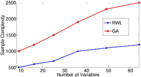
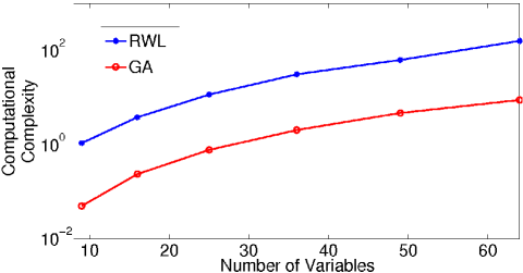
In the first experiment, we evaluate our algorithm on grids of various sizes. Fig. 3 compares the sample complexity and computational complexity of our algorithm to those of (Ravikumar et al., 2010) which will be henceforth referred to as RWL. Note that RWL is specifically tailored to the Ising model, and leverages this to yield lower sample complexity. Ours is a generic algorithm that can be used for any discrete graphical model, and thus requires more (but comparable) number of samples. It can be seen however that our algorithm is much faster than RWL.
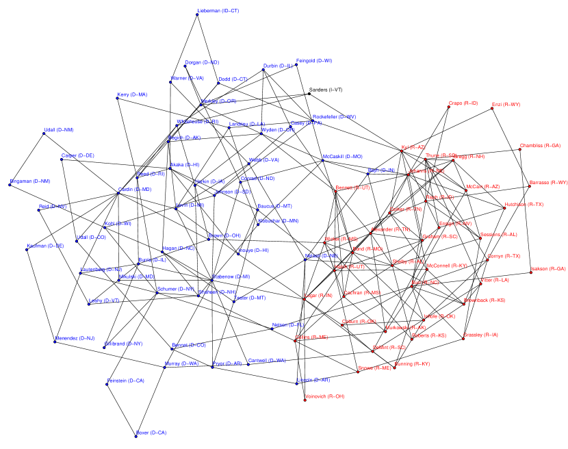
Finally, we present an application of our algorithm to model senator interaction graph using the senate voting records, following (Banerjee et al., 2008). A Yea vote is treated as a where as a Nay vote or absentee vote is treated as . To avoid bias, we only consider senators who have voted in a fraction of atleast of all the bills during the years 2009 and 2010. The output graph is presented in Fig. 4.
7 Discussion
We developed a simple greedy algorithm for Markov structure learning. The algorithm is simple to implement and has low computational complexity. We then showed that under some non-degeneracy, correlation decay, maximum degree and girth assumptions on the MRF, our algorithm recovers the correct graph structure with samples. We then specialize our conditions to prove a self-contained result for the most popular discrete graphical model - the Ising model.
The success of our algorithm can be further improved by post-processing via pruning. In particular, as mentioned, the neighborhood of a node as estimated by our algorithm always includes the true neighborhood – but it may also include spurious nodes. The latter can be then identified by checking each node of the estimated neighborhood, to see if it actually provides a reduction in conditional entropy over and above all the other nodes. Analysis of the improvement achieved by such a procedure is more challenging, but it may be likely that doing so will reveal an algorithm that can handle much larger degrees and smaller girths.
Acknowledgments
This work was partially supported by ARO grant W911NF-10-1-0360. We thank Jason K. Johnson for letting us use his graph drawing code for the senator graph.
References
- Abbeel et al. (2006) P. Abbeel, D. Koller, and A. Y. Ng. Learning factor graphs in polynomial time and sample complexity. J. Mach. Learn. Res., 7:1743–1788, 2006. ISSN 1532-4435.
- Anandkumar and Tan (2011a) A. Anandkumar and V. Y. F. Tan. High-Dimensional Gaussian Graphical Model Selection: Tractable Graph Families. Preprint, June 2011a.
- Anandkumar and Tan (2011b) A. Anandkumar and V. Y. F. Tan. High-Dimensional Structure Learning of Ising Models : Tractable Graph Families. Preprint, June 2011b.
- Banerjee et al. (2008) O Banerjee, L. El Ghaoui, and A. d’Aspremont. Model selection through sparse maximum likelihood estimation for multivariate gaussian or binary data. J. Mach. Learn. Res., 9:485–516, 2008. ISSN 1532-4435.
- Bento and Montanari (2009) Jose Bento and Andrea Montanari. Which graphical models are difficult to learn?, 2009. http://arxiv.org/abs/0910.5761.
- Bresler et al. (2008) G. Bresler, E. Mossel, and A. Sly. Reconstruction of markov random fields from samples: Some observations and algorithms. In APPROX ’08 / RANDOM ’08, pages 343–356, Berlin, Heidelberg, 2008. Springer-Verlag. ISBN 978-3-540-85362-6. doi: http://dx.doi.org/10.1007/978-3-540-85363-3˙28.
- Brush (1967) Stephen G. Brush. History of the Lenz-Ising model. Rev. Mod. Phys., 39(4):883–893, Oct 1967. doi: 10.1103/RevModPhys.39.883.
- Chow and Liu (1968) C. I. Chow and C. N. Liu. Approximating discrete probability distributions with dependence trees. IEEE Transactions on Information Theory, 14:462–467, 1968.
- Cover and Thomas (2006) Thomas M. Cover and Joy A. Thomas. Elements of Information Theory, 2nd Edition (Wiley Series in Telecommunications and Signal Processing). Wiley-Interscience, New York, NY, USA, 2006. ISBN 0471241954.
- El Karoui (2008) N. El Karoui. Operator norm consistent estimation of large-dimensional sparse covariance matrices. Annals of Statistics, 36(6):2717–2756, 2008.
- Furrer and Bengtsson (2007) R. Furrer and T. Bengtsson. Estimation of high-dimensional prior and posterior covariance matrices in kalman filter variants. Journal of Multivariate Analysis, 98(2):227–255, 2007.
- Jalali et al. (2011) A. Jalali, P. Ravikumar, V. Vasuki, and S. Sanghavi. On learning discrete graphical models using group-sparse regularization. In International Conference on Artificial Intelligence and Statistics (AISTATS) 14, 2011.
- Kamada and Kawai (1989) T. Kamada and S. Kawai. An algorithm for drawing general undirected graphs. Inf. Proc. Letters, 31(12):7–15, 1989.
- Lauritzen (1996) Steffen L. Lauritzen. Graphical Models. Oxford University Press, 1996. ISBN 0-19-852219-3.
- Netrapalli et al. (2010) P. Netrapalli, S. Banerjee, S. Sanghavi, and S. Shakkottai. Greedy learning of Markov network structure. In Communication, Control, and Computing (Allerton), 2010 48th Annual Allerton Conference on, pages 1295 –1302, Sept. 29 - Oct. 1 2010.
- Ravikumar et al. (2010) P. Ravikumar, M. W. Wainwright, and J. D. Lafferty. High-dimensional graphical model selection using -regularized logistic regression. Annals of Statistics, 38(3):1287–1319, 2010.
- Ravikumar et al. (2011) P. Ravikumar, M. W. Wainwright, G. Raskutti, and B. Yu. High-dimensional covariance estimation by minimizing -penalized log-determinant divergence. Electronic Journal of Statistics, 5:935–980, 2011.
- Santhanam and Wainwright (2009) Narayana P. Santhanam and Martin J. Wainwright. Information-theoretic limits of selecting binary graphical models in high dimensions, 2009. http://arxiv.org/abs/0905.2639.
- Zhou et al. (2010) S. Zhou, J. Lafferty, and L. Wasserman. Time varying undirected graphs. Machine Learning, 80:295–319, 2010.
Appendix
We will first prove the lemmas required for proving Proposition 3
Proof [Lemma 9] The proof is by construction. For each node , let . For the root node, let . For any other node , let be the parent of in the rooted tree with root . Define . Let and be the potential functions corresponding to and respectively. Then,
Since the potential functions are preserved by the bijections, so are the probabilities.
We will first prove the following lemma which will help us in proving Lemma 10.
Lemma 13
Consider a tree Ising graphical model with root , set of leaves and all positive edge parameters. Let be its probability distribution. Then, the quantity is monotonically increasing in . Moreover, is monotonically increasing in .
Proof For simplicity of notation, we define . Let us prove the above statement by induction on the depth of the tree. For a tree of depth , we have that
Since , increases when is changed from to .
Now, suppose the statement is true for all trees of depth upto . Consider a tree of depth , with root . Let be the set of children of . For every , let be the subtree rooted at with the same edge parameters as in and be the leaves of . Let be the probability measure corresponding to and . Then, the conditional probability of the root node can be written as
| (10) |
where , and and are independent of and . Since and , increases if increases. So, for any leaf node, if its value changes from to , the corresponding increases and hence increases, proving the induction claim.
Using the same induction argument as above and noting that , it can be seen that
is monotonically increasing in .
Proof [Lemma 10]
We know that for . Clearly any that maximizes
should either minimize or maximize . Note also that there is a one-one correspondence between such
configurations (i.e., for every maximizing configuration, there exists a minimizing configuration such that
both of them maximize ).
From Lemma 13, we know that maximizes and by symmetry this should be the same as
and equal .
So, we can conclude that is maximized by .
Lemma 14
Consider a tree Ising model with root node , set of leaves and maximum degree . Let be its probability measure. Suppose the absolute values of the edge parameters are bounded by . Then, we have that .
Proof Using Lemmas 9, 10 and 13, we can assume without loss of generality that the parameters on all the edges are positive and equal to (which is the maximum possible value), consider a complete D-ary tree and concentrate on . For simplicity of notation, let . For a tree of depth , let . We have that
Using some algebraic manipulations and substituting the value of , we obtain
and the result follows.
We need the following lemma to prove Lemma 11.
Lemma 15
Consider a tree Ising model , with root node , set of leaves and maximum degree . Let be its probability measure. Suppose the absolute values of the edge parameters are bounded by . Then, such that is a child of , we have that .
Proof
Using Lemma 9
we can assume without loss of generality that the parameters on all the edges are positive.
can take values . For each of those values, the value of that
maximizes
either maximizes or minimizes
. Noting from (a slight extension to) Lemma 13
that is monotonic in , it suffices to consider the eight possibilities
.
We show how to calculate the above value for . Interested readers can check that
the conclusions below apply to all the other cases as well.
Using Lemma 13, we can assume that the parameters
on all the edges except the edge are equal to and consider
a complete D-ary tree. Let .
We know that .
Let be the depth of the tree and .
We have
where is as defined in Lemma 14.
Using some algebraic manipulations, it can be shown that . Using Lemma 14 finishes the proof.
Proof [Proposition 3] Let . Let be a set that separates and such that . Let be the component of nodes containing when the graph is separated by . We know that the induced subgraph on is a tree. Applying Lemma 11 on this tree and using Lemma 8, we obtain . Since is a weighted average of for various , we have
The result then follows since is a weighted average of .
Proof [Lemma 12] Let the graphical model be denoted by , denote the potential on edge when and and denote the potential due to all edges with both vertices in when . In the following, we assume that the girth of the graph is . Consider a node and a subset of its neighbors and a node which is a neighbor of . We know that the pairwise potentials satisfy . Let and consider the graph with the same potentials on all edges as in . Let and choose any other set . Let and be the probability mass functions corresponding to and respectively. Similarly let and be the distance between and in and respectively. Suppose further that . Then, . Note that,
| (11) |
where is an appropriate normalizing constant. Note that . It follows from this that . Using (11), the hypothesis that an Ising model has almost exponential correlation decay, we obtain the following inequalities after some algebraic manipulations,
| (12) |
| (13) |
.Combining (12) and (13), we obtain
and subsequently by marginalizing, we obtain
Let . Since , we have that . So, separating and in such that . Then,
| (14) |
where the last inequality follows from the lower bound on girth in the hypothesis.
Now consider the graph where . Let the potentials on the edges in be the same as those in and denote the corresponding probability mass function by . Clearly, we have the following relation between and .
where is an appropriate normalizing constant. Using (14) and the symmetry of the Ising model (i.e., for ), we obtain
after some algebraic manipulations. Similarly, we also have
which implies
Finally, letting , we have,
So, we have shown that under the given conditions, an Ising model satisfies (3) with . It is straightforward to note that the above proof can also be used to show that the Ising model also satisfies (4) with the same , completing the proof of the lemma.