On non-stationary Lamé equation from WZW model and spin-1/2 XYZ chain

Abstract:

We study the link between WZW model and the spin-1/2 XYZ chain. This is achieved by comparing the second-order differential equations from them. In the former case, the equation is the Ward-Takahashi identity satisfied by one-point toric conformal blocks. In the latter case, it arises from Baxter’s $TQ$ relation. We find that the dimension of the representation space w.r.t. the $V$-valued primary field in these conformal blocks gets mapped to the total number of chain sites. By doing so, Stroganov’s “The Importance of being Odd” (cond-mat/0012035) can be consistently understood in terms of WZW model language. We first confirm this correspondence by taking a trigonometric limit of the XYZ chain. That eigenstates of the resultant two-body Sutherland model from Baxter’s $TQ$ relation can be obtained by deforming toric conformal blocks supports our proposal.

1 Introduction

About twenty years ago, a series of pioneering papers [1, 2, 3] established an intriguing connection between XXX Gaudin and Wess-Zumino-Witten (WZW) models. That is, the problem of diagonalizing commuting Hamiltonians of XXX Gaudin model is translated into solving Knizhnik-Zamolodchikov (KZ) equations defined on ${\bf CP}^{1}$ [6]. Indeed, Bethe roots of Bethe ansatz equations in the inhomogeneous XXX Gaudin model turn out to constitute solutions to KZ equations at critical level. Later on, the authors of [7, 8, 9] further extended this direction to the elliptic case. Certainly, their works are based on important investigations on both XYZ Gaudin model [10] and conformal field theory (CFT) on elliptic curves [11, 12, 13].

In this letter, we would like to add into the above picture a novel element: a relation between WZW model and the spin-1/2 XYZ chain as depicted in Fig. 1. By examining non-stationary Lamé equations on both sides we are able to interpret Stroganov’s proposal (The Importance of being Odd) [14] from the viewpoint of CFT under the dictionary listed in Table 1.

Table 1: Dictionary

	Spin-1/2 XYZ chain	WZW model
non-stationary Lamé eq.	Baxter’s $TQ$ eq.	KZB eq. (WT identity)
coupling const.	site number	dim. of  $\mathfrak{sl}_{2}$ rep.
time	anisotropy parameter	torus moduli
space	spectral parameter	Cartan moduli

More precisely, in [15] Razumov and Stroganov made a conjecture about the exact ground-state eigenvalue of the transfer matrix in the spin-1/2 XYZ chain. This conjecture holds only for the odd chain site number and plays a crucial role in deriving the aforementioned Lamé equation [16]. On the other hand, one-point toric conformal blocks exist only when the dimension of the $\mathfrak{sl}_{2}$ representation space w.r.t. the inserted primary field is odd. It is thus tempting to connect these two facts through Table 1. As a test, we perform a trigonometric degeneration of the XYZ chain. Consequently, that eigenstates of Sutherland-type equations descending from Baxter’s $TQ$ relation reduce to Schur polynomials under certain limit is well reflected by imposing a corresponding constraint on WZW toric conformal blocks.

We organize this letter as follows. In the next section, we review how Lamé equations emerge from the spin-1/2 XYZ chain as a result of Baxter’s $TQ$ relation. We compare it with Knizhnik-Zamolodchikov-Bernard (KZB) equations in section 3. In section 4, we justify this comparison via a trigonometrical reduction. Finally, a summary is given in section 5.

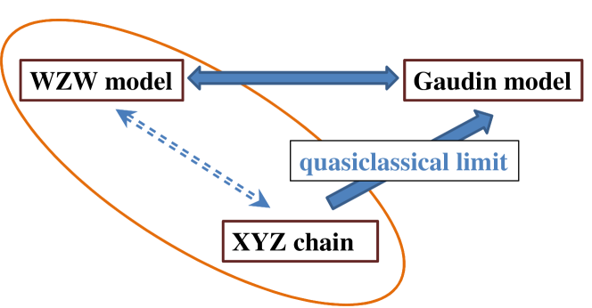
Figure 1: Two solid arrows above represent the known connections between spin-chain and WZW models. The encircled part indicates the novel relationship under consideration.

2 Spin-1/2 XYZ chain side

Let us briefly review how the non-stationary Lamé equation is obtained from Baxter’s $TQ$ equation of the spin-1/2 XYZ chain [15, 16] whose Hamiltonian is described by

$$H_{XYZ}=\sum_{n=1}^{M}\biggl{\{}J_{X}S_{n}^{X}S_{n+1}^{X}+J_{Y}S_{n}^{Y}S_{n+1}^{Y}+J_{Z}S_{n}^{Z}S_{n+1}^{Z}\biggl{\}}.$$ (1)

Here, $S_{n}^{X,Y,Z}=\sigma_{n}^{X,Y,Z}/2$ ($\sigma_{n}^{X,Y,Z}$: Pauli matrix) acts on the $n$-th site and the periodic boundary condition $S_{M+1}^{X,Y,Z}=S_{1}^{X,Y,Z}$ is imposed. Recall that the terminology XYZ means anisotropic $J$’s while the partial anisotropy $J_{X}=J_{Y}\neq J_{Z}$ (isotropy $J_{X}=J_{Y}=J_{Z}$) case is called the XXZ (XXX) chain. $H_{XYZ}$ acts on the tensor product $V_{1}\otimes V_{2}\otimes\cdots\otimes V_{M}$ where each $V_{n}$ is a complex two-dimensional space ${\bf C}^{2}$ spanned by the up- and down-spin states.

A fundamental ingredient in integrable spin-chain models is the $R$ matrix. For the spin-1/2 XYZ chain, its matrix elements are given by

$$R(z)=\begin{pmatrix}a(z)&0&0&d(z)\\ 0&b(z)&c(z)&0\\ 0&c(z)&b(z)&0\\ d(z)&0&0&a(z)\end{pmatrix}$$

where (nome: $q=e^{\pi i\tau}$)

$$a(z) =\rho\theta_{4}(2\eta|q)\theta_{4}(z|q)\theta_{1}(z+2\eta|q),\ \ \ \ b(z)=\rho\theta_{4}(2\eta|q)\theta_{1}(z|q)\theta_{4}(z+2\eta|q),$$

$$c(z) =\rho\theta_{1}(2\eta|q)\theta_{4}(z|q)\theta_{4}(z+2\eta|q),\ \ \ \ d(z)=\rho\theta_{1}(2\eta|q)\theta_{1}(z|q)\theta_{1}(z+2\eta|q),$$

$$\rho =\frac{2}{\theta_{2}(0|q^{\frac{1}{2}})\theta_{4}(0|q)},$$

$$\theta_{1}(z|q) =-i\sum_{n\in{\bf Z}}(-1)^{n}q^{(n+\frac{1}{2})^{2}}\mathrm{e}^{(2n+1)\pi iz},\ \ \ \ ~{}~{}~{}~{}~{}~{}~{}\theta_{2}(z|q)=\sum_{n\in{\bf Z}}q^{(n+\frac{1}{2})^{2}}\mathrm{e}^{(2n+1)\pi iz},$$

$$\theta_{3}(z|q) =\sum_{n\in{\bf Z}}q^{n^{2}}\mathrm{e}^{2n\pi iz},\ \ \ \ ~{}~{}~{}~{}~{}~{}~{}~{}~{}~{}~{}~{}~{}~{}~{}~{}~{}~{}~{}~{}~{}~{}~{}~{}~{}~{}~{}~{}\theta_{4}(z|q)=\sum_{n\in{\bf Z}}(-1)^{n}q^{n^{2}}\mathrm{e}^{2n\pi iz}.$$

Note that $(q,\eta)$ determines the anisotropy parameters of the XYZ chain through Jacobi’s elliptic functions:

$$J_{X}=1+{\bf k}\mathrm{sn}^{2}(\pi\eta,{\bf k}),\ \ \ J_{Y}=1-{\bf k}\mathrm{sn}^{2}(\pi\eta,{\bf k}),\ \ \ J_{Z}=\mathrm{cn}(\pi\eta,{\bf k})\mathrm{dn}(\pi\eta,{\bf k}),\ \ \ {\bf k}=\frac{\theta^{2}_{2}(0|q)}{\theta^{2}_{3}(0|q)}.$$

Also, $z$ denotes the spectral parameter which plays an important role in quantum integrable models. When $q\to 0$, due to ${\bf k}\to 0$ as well as

$$\mathrm{sn}(\pi\eta,{0})=\sin\pi\eta,\ \ \ \ \ \ \mathrm{cn}(\pi\eta,{0})=\cos\pi\eta,\ \ \ \ \ \ \mathrm{dn}(\pi\eta,{0})=1,$$

one yields a XXZ chain with

$$J_{X}=J_{Y}=1,\ \ \ \ \ \ J_{Z}=\cos\pi\eta.$$

Remark that $2J_{Z}={\bf q}+{\bf q}^{-1}$ where ${\bf q}=\exp(\pi i\eta)$ is referred to as the deformation parameter ${\bf q}$ of the quantum group $U_{\bf q}({\mathfrak{sl}}_{2})$.

In fact, three $R$-matrices acting on $V_{1}\otimes V_{2}\otimes V_{3}$ satisfy the famous Yang-Baxter relation:

$$R_{12}(z)R_{13}(z+w)R_{23}(w)=R_{23}(w)R_{13}(z+w)R_{12}(z).$$

The subscript of, say, $R_{13}(z)$ means that it acts on $V_{1}\otimes V_{3}$. From these $R$-matrices, one can construct the monodromy matrix $T_{a}(z)$ acting on $V_{a}\otimes(V_{1}\otimes\cdots\otimes V_{M})$:

$$T_{a}(z)=R_{aM}(z)\cdots R_{a1}(z)=\left(\begin{array}[]{cc}A(z)&B(z)\\ C(z)&D(z)\end{array}\right).$$ (4)

One can further yield the transfer matrix ${\mathcal{T}}(z)=\mathrm{tr}_{a}T_{a}(z)$ by performing a trace over the auxiliary space $V_{a}$. Utilizing the above Yang-Baxter relation repeatedly, one arrives at the so-called $RTT$ relation:

$$R_{ab}(z-w)T_{a}(z)T_{b}(w)=T_{b}(w)T_{a}(z)R_{ab}(z-w),$$

from which the commutativity of transfer matrices follows:

$$[\mathcal{T}(z),\mathcal{T}(w)]=0.$$

Let us briefly explain why there exists a common ${\bf q}$ between the XXZ Hamiltonians $H_{XXZ}$ and $U_{\bf q}({\mathfrak{sl}}_{2})$ encountered above. First, one can construct the XXZ transfer matrix from a product of $R$-matrices of the affine quantum group $U_{\bf q}(\widehat{\mathfrak{sl}}_{2})$. Then, in order to derive $H_{XXZ}$ the standard way is to take the logarithmic derivative of the XXZ transfer matrix.

2.1 Baxter’s $TQ$ relation as non-stationary Lamé equation

Baxter’s $Q$-operator method is a powerful tool for finding the eigenvalue of transfer matrices. Let us briefly sketch his approach here. One prepares a local matrix $S_{aj}(z)$ which acts on $W_{a}\otimes V_{j}$ where $W_{a}=\mathbf{C}^{L}$ when $\exp(\pi i\eta L)=1$. From $S_{aj}(z)$ we construct a global matrix

$$Q_{a}(z)= S_{aM}(z)\cdots S_{a1}(z)$$

acting on $W_{a}\otimes(V_{1}\otimes\cdots\otimes V_{M})$. Baxter’s $Q$-operator is defined by $\mathcal{Q}(z)=\mathrm{tr}_{W_{a}}Q_{a}(z)$ which acts also on the previous $V=V_{1}\otimes\cdots\otimes V_{M}$. Baxter’s idea was to consider the product of $\mathcal{T}(z)$ and $\mathcal{Q}(z)$

$$\mathcal{T}(z)\mathcal{Q}(z) =\mathrm{tr}_{V_{a}\otimes W_{a^{\prime}}}\Bigg{\{}\prod_{j=1}^{M}R_{aj}(z)S_{a^{\prime}j}(z)\Bigg{\}}$$

$$=\mathrm{tr}_{V_{a}\otimes W_{a^{\prime}}}\Bigg{\{}\prod_{j=1}^{M}UR_{aj}(z)S_{a^{\prime}j}(z)U^{-1}\Bigg{\}}$$

followed by a gauge transformation: $R_{aj}(z)S_{a^{\prime}j}(z)\to UR_{aj}(z)S_{a^{\prime}j}(z)U^{-1}$ such that the latter becomes a triangular matrix via a suitable $U$. By doing so, both eigenvalues of $\mathcal{T}(z)$ and $\mathcal{Q}(z)$ are shown to satisfy Baxter’s $TQ$ relation [17]

$${\mathcal{T}}(z)\mathcal{Q}(z)=\phi(z-\frac{\eta}{2})\mathcal{Q}(z+\eta)+\phi(z+\frac{\eta}{2})\mathcal{Q}(z-\eta)$$ (5)

with $\phi(z)=\theta_{1}^{M}(z|q)$.

At the Razumov-Stroganov point $\eta=1/3$ [15], a particularly simple expression for the ground-state eigenvalue of $\mathcal{T}(z)$ was conjectured to be $\phi(z)$ [14, 15, 24]. Their conjecture holds only when the number of chain sites is odd: $M=2n+1$ ($n\in\mathbf{Z}_{\geq 0}$). Inserting this ${\mathcal{T}}(z)$ into (5), Bazhanov and Mangazeev [16] managed to show that $Q$-operators dressed by

$$\Psi_{\pm}^{(8\mathrm{vertex})}(z,q,n)=\frac{\theta_{1}^{2n+1}(z|q)}{\theta_{1}^{n}(3z|q^{3})}\mathcal{Q}_{\pm}(z,q,n)$$

satisfy the non-stationary Lamé equation:

$$6q\frac{\partial}{\partial q}\Psi_{\pm}^{(8\mathrm{vertex})}(z,q,n)=\frac{1}{\pi^{2}}\left\{-\frac{\partial^{2}}{\partial z^{2}}+{9}n(n+1)\wp(3z|q^{3})+c(q,n)\right\}\Psi_{\pm}^{(8\mathrm{vertex})}(z,q,n).$$ (6)

Let two half-periods of Weierstrass’s elliptic function $\wp(z|q)\equiv\wp(z|\omega_{1},\omega_{2})$ be $(\omega_{1},\omega_{2})\equiv(1/2,\tau/2)$. Then,

$$\wp(z|q) =-\zeta^{\prime}(z|q),$$

$$\zeta(z|q) =\frac{\theta_{1}^{\prime}(z|q)}{\theta_{1}(z|q)}+2\eta_{1}(q)z,$$

$$\eta_{1}(q) =4\pi^{2}\left(\frac{1}{24}-\sum_{n=1}^{\infty}\frac{nq^{n}}{1-q^{n}}\right)=-\frac{1}{6}\frac{\theta_{1}^{\prime\prime\prime}(0|q)}{\theta_{1}^{\prime}(0|q)},$$

$$c(q,n) =18n(n+1)\eta_{1}(q^{3}).$$

In terms of the new variable $s=3z$, one can rewrite (6) into

$$\frac{2}{3}q\frac{\partial}{\partial q}\Psi_{\pm}^{(8\mathrm{vertex})}(s/3,q,n)=\frac{1}{\pi^{2}}\left\{-\frac{\partial^{2}}{\partial s^{2}}+n(n+1)\Big{(}\wp(s|q^{3})+2\eta_{1}(q^{3})\Big{)}\right\}\Psi_{\pm}^{(8\mathrm{vertex})}(s/3,q,n).$$ (7)

We can replace $2q{\partial}/3{\partial q}$ by $2{\partial}/\pi i{\partial\bar{\tau}}$ with $3\tau=\bar{\tau}$.

3 WZW model side

Our goal is to see the appearance of (6) within the context of WZW model and then interpret Stroganov’s claim geometrically.

3.1 Affine Lie algebra

The conformal symmetry here will be realized by means of the level-$k$ affine Lie algebra $\widehat{\mathfrak{g}}$. In general, the integrable irreducible $\widehat{\mathfrak{g}}$-module $L_{k,\lambda}$ is characterized by a set of non-negative highest weights ${\lambda_{a}}$ $(a=0,\cdots,r={\rm rank})$ w.r.t. $\mathfrak{g}$ (simple finite-dimensional Lie algebra) where $\lambda_{0}=k-(\theta,\lambda)\geq 0$. Symbolically,

$$\lambda_{a}\in P^{k}_{+}=\{\lambda_{a}\in P_{+}~{}|~{}0\leq(\theta,\lambda)\leq k\},~{}~{}~{}~{}~{}~{}~{}~{}a=1,\cdots,r.$$

$L_{k,\lambda}$ with all null states being decoupled forms an unitary representation of $\widehat{\mathfrak{g}}$. Let us proceed to explain various notations used above.

We focus only on the $A_{N-1}$-type Lie algebra $\mathfrak{sl}_{N}$ whose $N^{2}-1$ generators can get triangularly decomposed into $\mathfrak{sl}_{N}=\mathfrak{n}_{-}\oplus\mathfrak{h}\oplus\mathfrak{n}_{+}$ ($\mathfrak{h}$: Cartan subalgebra, $r={\rm dim}\mathfrak{h}$). Consider its $(N^{2}-1)$-dimensional adjoint representation labeled by a root system $\Delta=\Delta_{+}\cup\Delta_{-}$, i.e. a set of vectors in a $r$-dimensional lattice. Given one positive (non-zero) root vector $\alpha\in\Delta_{+}$, we can choose $E_{\alpha}=E_{i,j}\in\mathfrak{n}_{+}$ ($i<j$). Note that $E_{i,j}$ is an $N\times N$ matrix with its $(i,j)$-th entry unity and zero otherwise. Take for example $\Phi={\rm diag}(x_{1},\cdots,x_{N})\in\mathfrak{h}~{}({\rm subject~{}to}~{}x_{1}+\cdots+x_{N}=0$). There holds

$$[\Phi,E_{\alpha}]=\alpha(\Phi)E_{\alpha},~{}~{}~{}~{}~{}~{}~{}~{}\alpha(\Phi)=x_{i}-x_{j}.$$ (8)

Because all roots are located in a $r$-dimensional lattice and only $r$ of them are independent, let ${\bar{\alpha}}_{a}$ be simple roots such that $\alpha=\sum^{r}_{a=1}m_{a}{\bar{\alpha}}_{a}\in\Delta_{+}$ if $m_{a}\in{\bf Z}_{\geq 0}$. Generators in Cartan subalgebra are normalized by the length constraint $(\alpha,\alpha)=2$ where the inner product is the usual one. In other words, given an orthonormal basis $\{e_{1},\cdots,e_{N}\}$ obeying $(e_{i},e_{j})=\delta_{ij}$ let $\alpha\equiv e_{i}-e_{j}\in\Delta$ $(1\leq i\neq j\leq N)$. For positive roots in $\Delta_{+}$, $i<j$. For simple roots, $j=i+1$. Consequently, we are led to

$$[E_{\alpha},E_{-\alpha}]=E_{i,i}-E_{j,j}\equiv H_{\alpha},~{}~{}~{}~{}~{}~{}~{}~{}[H_{\alpha},E_{\alpha}]=\alpha(H_{\alpha})E_{\alpha}=2E_{\alpha},$$

which implies that the weight of each root vector is just encoded in $\Delta$.

From now on, we adopt the so-called Weyl-Cartan basis for $\mathfrak{g}$. That is, define ${\bf H}=(H_{1},\cdots,H_{r})\in\mathfrak{h}$ such that the highest weight state $|\lambda\rangle$ satisfies $H_{a}|\lambda\rangle=\lambda_{a}|\lambda\rangle$. When it comes to roots, for $\alpha=({\bf\alpha}_{1},\cdots,{\bf\alpha}_{r})\in\Delta_{+}$ one has under this basis

$$[H_{a},H_{b}]=0,~{}~{}~{}~{}~{}~{}~{}~{}[E_{\alpha},E_{-\alpha}]=\sum^{r}_{a=1}{\bf\alpha}_{a}^{\vee}{H_{a}},~{}~{}~{}~{}~{}~{}~{}~{}[H_{a},E_{\alpha}]={\bf\alpha}_{a}E_{\alpha}.$$ (9)

Here, ${\alpha}^{\vee}=2\alpha/(\alpha,\alpha)$ and again $(\alpha,\alpha)=2$ is imposed as a normalization of ${\bf H}$ where the inner product $(\alpha,\alpha)=\sum_{a}{\alpha}_{a}\alpha_{a}$.

Let ${\bar{\alpha}}^{\vee}$’s be simple coroots represented by

$${\bar{\alpha}}^{\vee}_{a}=\sum^{r}_{b=1}A_{ab}\Lambda_{b},~{}~{}~{}~{}~{}~{}~{}~{}A_{ab}=({\bar{\alpha}}_{a},{\bar{\alpha}}_{b}^{\vee}):~{}{\rm{Cartan~{}matrix}}.$$

A set of fundamental weights $\{\Lambda_{a}\}$ is used to express the highest weight vector as $\lambda=\sum_{a}\lambda_{a}\Lambda_{a}$ with $({\bar{\alpha}}_{a}^{\vee},\Lambda_{b})=\delta_{ab}$. The level $k$ of $\widehat{\mathfrak{sl}}_{N}$ is given by

$$k=\lambda_{0}+(\theta,\lambda)=\sum^{r}_{a=0}\lambda_{a},~{}~{}~{}~{}~{}~{}~{}~{}\theta=\sum^{r}_{a=1}{\bf a}^{\vee}_{a}{\bar{\alpha}}_{a}^{\vee},=\sum^{r}_{a=1}{\bar{\alpha}}_{a}^{\vee},~{}~{}~{}~{}~{}~{}~{}~{}{\bf a}^{\vee}_{a}:~{}{\rm{colabel}},$$

where $\kappa=k+h^{\vee}$ ($h^{\vee}=\sum^{r}_{a=0}{\bf a}^{\vee}_{a}$: dual Coxeter number). For the $A$-type Lie algebra, ${\bf a}^{\vee}_{0}={\bf a}^{\vee}_{a}=1$. While the level $k$ goes to infinity, the integrable irreducible $\widehat{\mathfrak{g}}$-module reduces to that of ${\mathfrak{g}}$.

3.2 KZB equation

We move to discuss correlation functions in WZW model. Of interest are their chiral parts, conformal blocks, satisfying Knizhnik-Zamolodchikov equations [6, 11]. However, it is necessary for us to first get familiar with constructing Virasoro algebra from affine Lie ones.

Let $J^{I}_{n}$ ($n\in\mathbf{Z}$, $I,J=1,\cdots,{\rm dim}{\mathfrak{g}}$) be generators of the affine Lie algebra $\widehat{\mathfrak{g}}=\mathfrak{g}\otimes{\mathbf{C}}[z,z^{-1}]\oplus c{\mathbf{C}}$ whose central extension is $c={k{\text{dim}}\mathfrak{g}}/\kappa$ where

$$12\rho^{2}=h^{\vee}{\rm dim}{\mathfrak{g}},~{}~{}~{}~{}~{}~{}~{}~{}\rho=\sum^{r}_{a=1}\Lambda_{a}=\sum_{\alpha\in\Delta_{+}}\frac{\alpha}{2}:~{}{\rm Weyl~{}vector}.$$

According to Sugawara’s construction, the generator of Virasoro algebra can be expressed via $J^{I}_{n}$:

$$2\kappa L_{n}=\sum_{m\in{\mathbf{Z}}}g_{IJ}:J_{n-m}^{I}J_{m}^{J}:=g_{IJ}(\sum_{m<0}J_{m}^{I}J_{n-m}^{J}+\sum_{m\geq 0}J_{n-m}^{I}J_{m}^{J})$$

where $g_{IJ}$ is the inverse of $g^{IJ}=K({\mathfrak{g}}_{I},{\mathfrak{g}}_{J})$ called Killing form:

$$K(H_{a},H_{b})=\delta_{ab},~{}~{}~{}~{}~{}~{}~{}~{}K(E_{\alpha},E_{-\alpha})=\frac{2}{\alpha^{2}},~{}~{}~{}~{}~{}~{}~{}~{}K(\cdot,\cdot)={\rm zero~{}otherwise}.$$

In particular, $\kappa L_{0}$ is translated into the quadratic Casimir operator $\Omega$ of ${\mathfrak{g}}$:

$$\Omega=\frac{1}{2}\sum_{a=1}^{r}H_{a}^{2}+\frac{1}{4}\sum_{\alpha\in\Delta_{+}}{\alpha^{2}}(E_{\alpha}E_{-\alpha}+E_{-\alpha}E_{\alpha}),~{}~{}~{}~{}~{}\alpha^{2}=(\alpha,\alpha)$$ (10)

when applied to the highest weight state $|\lambda\rangle$. Following (9), we see that $L_{0}$ actually measures the conformal dimension $\Delta_{\lambda}$ of $|\lambda\rangle$ in the module $L_{k,\lambda}$:

$$\Delta_{\lambda}=\frac{(\lambda,\lambda+2\rho)}{2\kappa}$$ (11)

where the inner product is taken w.r.t. the preceding Weyl-Cartan basis.

Our main concern are KZB equations which look like

$$\kappa\frac{\partial}{2\pi i\partial\tau^{\prime}}\Psi=\frac{1}{4}H_{0}\Psi,~{}~{}~{}~{}~{}~{}H_{0}=-\frac{1}{2\pi^{2}}\sum_{a=1}^{r}\partial_{u_{a}}\partial_{u_{a}}+2\sum_{\alpha\in\Delta}p(e^{\alpha(U)})E_{\alpha}E_{-\alpha},$$ (12)

where

$$U=2\pi i~{}\sum_{a=1}^{r}u_{a}H_{a},~{}~{}~{}~{}~{}~{}p(t)=-\sum_{m\in{\bf Z}}\frac{q^{\prime m}t}{(1-q^{\prime m}t)^{2}},~{}~{}~{}~{}~{}~{}q^{\prime}=e^{2\pi i\tau^{\prime}}$$ (13)

and ${\alpha(U)}$ is defined in (8). Certainly, (12) is derived by applying the Ward-Takahashi identity associated with the energy-momentum tensor $T(z)=\sum_{n\in{\mathbf{Z}}}z^{-n-2}L_{n}$ to one-point toric conformal blocks $\Psi$:

$$\Psi={\rm Tr}_{L_{k,\lambda}}~{}\Big{(}q^{\prime L_{0}-\frac{c}{24}}e^{U}v_{\ell}(z)\Big{)},~{}~{}~{}~{}~{}~{}\ell\in P^{k}_{+},~{}~{}~{}~{}~{}~{}c=\frac{k{\text{dim}}\mathfrak{g}}{\kappa}.$$ (14)

Notice that for $\mathfrak{sl}_{2}$ the primary field $v_{\ell}(z)$ is $V$-valued (taking its value in $V$) and acted on by $\rho_{\ell}$ given certain spin-$\ell/2$ $\mathfrak{sl}_{2}$ representation ($\rho_{\ell},V_{\ell}$). Still, the marked point $z$ located on the torus (complex moduli $\tau^{\prime}$) can be sent to zero because $\Psi$ satisfies

$$\Big{(}z\frac{\partial}{\partial z}+\rho_{\ell}(\kappa^{-1}\Omega)\Big{)}\Psi=0.$$ (15)

By definition, without any $v_{\ell}(z)$ inserted $\Psi$ reduces to the affine character associated with the integrable module $L_{k,\lambda}$:

$$\Psi\to\chi={\rm Tr}_{L_{k,\lambda}}~{}\Big{(}q^{\prime L_{0}-\frac{c}{24}}e^{U}\Big{)}.$$ (16)

Let us pause for a while to discuss the $V$-valuedness of $v_{\ell}(z)$. This can be done twofold. First, define $v(z)\equiv v(\zeta|z)$ which depends additionally on an internal coordinate $\zeta$. Its OPE with some $\widehat{\mathfrak{sl}}_{2}$-current field $J^{I}(w)$ reads

$$J^{I}(w)v(\zeta|z)\sim\frac{1}{w-z}{\cal D}^{I}(\zeta)v(\zeta|z),~{}~{}~{}~{}~{}~{}{\cal D}^{I}(\zeta)v(\zeta|z)\equiv\rho(J^{I})v(z).$$

Second, we resort to Wakimoto’s representation. Introduce the primary field corresponding to the $\widehat{\mathfrak{sl}}_{2}$ highest weight state $|\ell\rangle$ in terms of a chiral free boson $\varphi(z)$:

$$|\ell\rangle~{}\to~{}:\exp(\ell/\sqrt{2})\varphi(z):$$

whose conformal dimension $\Delta_{\ell}$ is just computed in (11) with $\lambda\to\ell$. Instead of the additional $\zeta$-dependence, one prepares another chiral free field $\gamma(z)$ and constructs the full ${\mathfrak{sl}}_{2}$ spin-$\ell/2$ multiplet which contains

$$\gamma(z)^{\ell/2-m}:\exp(\ell/\sqrt{2})\varphi(z):,~{}~{}~{}~{}~{}~{}m=-\ell/2,\cdots,\ell/2.$$ (17)

Then, $v_{\ell}(z)$ can be identified with one of them.

From (14) we realize that the role of $v_{\ell}(z)$ is an intertwiner, i.e. $v_{\ell}(z):~{}L_{k,\lambda}\to L_{k,\lambda}\otimes V[0]$. Here, $V[0]$ stands for the one-dimensional zero-weight subspace of $V_{\ell}$, ($\ell+1$)-dimensional ${\mathfrak{sl}}_{2}$-module. Due to the Ward-Takahashi identity w.r.t. $\widehat{\mathfrak{sl}}_{2}$-current fields applied to $\Psi$, we see ($H$: ${\mathfrak{sl}}_{2}$ Cartan generator)

$$\rho_{\ell}(H)\Psi=0.$$ (18)

This explains why $v_{\ell}(z)$ belongs to the zero-weight subspace $V[0]\subset V_{\ell}$.

3.3 $H_{0}$

Let us describe $H_{0}$ in (12) in more detail. We want to look into the function $p(t)$ [7, 9, 25, 26] inside $H_{0}$. By using Weierstrass’s $\wp$-function it gets expressed by ($t=e^{2\pi iw}$)

$$p(t)=-\frac{t}{(1-t)^{2}}-\sum_{m\neq 0}\frac{q^{\prime m}t}{(1-q^{\prime m}t)^{2}},$$

$$4\pi^{2}p(t)=-\partial_{w}^{2}\log\theta_{1}(w|q^{\prime\frac{1}{2}})=\wp(w|q^{\prime\frac{1}{2}})+2\eta_{1}(q^{\prime\frac{1}{2}}).$$ (19)

Here, $\wp$, $\theta_{1}$ and $\eta_{1}$ follow the same convention adopted in section 2. Eq. (3.3) is explained as below. Because $p(t)$ has order-two poles at $\{q^{\prime m}\}_{m\in{\bf Z}}$ and satisfies the periodicity condition $p(q^{\prime}t)=p(t)$, it can be rewritten into the form

$$p(t)=-\frac{t}{(1-t)^{2}}-\sum_{m>0}\left\{\frac{q^{\prime m}t}{(1-q^{\prime m}t)^{2}}+\frac{q^{\prime m}t^{-1}}{(1-q^{\prime m}t^{-1})^{2}}\right\}.$$

Recalling $t=e^{2\pi iw}$ we find the first term becomes

$$-\frac{t}{(1-t)^{2}}=\frac{1}{4\sin^{2}(\pi w)},$$

and other terms become

$$-\frac{q^{\prime m}t}{(1-q^{\prime m}t)^{2}}-\frac{q^{\prime m}t^{-1}}{(1-q^{\prime m}t^{-1})^{2}}=-2q^{\prime m}\frac{\cos(2\pi w)(1+q^{\prime 2m})-2q^{\prime m}}{\big{(}1-2q^{\prime m}\cos(2\pi w)+q^{\prime 2m}\big{)}^{2}}.$$

On the other hand, based on the product representation of $\theta_{1}(w|q^{\prime\frac{1}{2}})$:

$$\theta_{1}(w|q^{\prime\frac{1}{2}})=2q^{\prime\frac{1}{8}}\sin(\pi w)\prod_{m>0}(1-q^{\prime m})\big{(}1-2q^{\prime m}\cos(2\pi w)+q^{\prime 2m}\big{)}$$

we have

$$-{\partial_{w}^{2}}\log\theta_{1}(w|q^{\prime\frac{1}{2}})=\frac{\pi^{2}}{\sin^{2}(\pi w)}-\sum_{m>0}8\pi^{2}q^{\prime m}\frac{\cos(2\pi w)(1+q^{\prime 2m})-2q^{\prime m}}{\big{(}1-2q^{\prime m}\cos(2\pi w)+q^{\prime 2m}\big{)}^{2}}.$$

Combined with

$$-{\partial_{w}^{2}}\log\theta_{1}(w|q^{\prime\frac{1}{2}})=\wp(w|q^{\prime\frac{1}{2}})+2\eta_{1}(q^{\prime\frac{1}{2}}),$$

we go back to (3.3). To explicitly evaluate $e^{\alpha(U)}$ for $p(t)$, we resort to (8). Generally, in the case of $\mathfrak{sl}_{N}$

$$\frac{1}{2\pi i}U=\sum^{r}_{a=1}u_{a}H_{a}={\rm diag}(y_{1},\cdots,y_{N}),~{}~{}~{}~{}~{}~{}\sum^{N}_{i=1}y_{i}=0.$$

Due to $(\alpha,\alpha)=2$ as stressed, one sees $\alpha(U)=2\pi i\sqrt{2}u_{1}$ and $w\to\sqrt{2}u_{1}\equiv u$ for $\mathfrak{sl}_{2}$.

Finally, we want to determine the eigenvalue of $E_{\alpha}E_{-\alpha}$ in (12) which acts on $V[0]\subset V_{\ell}$ of the primary field $v_{\ell}(z)$. Since $V[0]={\bf C}$ is one-dimensional, in view of (17) one can assume that it is spanned by some monomial like $(L_{1}\cdots L_{N})^{\xi}$. Furthermore, for $\mathfrak{sl}_{N}$ there exists the following representation:

$$E_{\alpha}\equiv E_{ij}=L_{i}\frac{\partial}{\partial L_{j}},~{}~{}~{}~{}~{}~{}i\neq j=1,\cdots N,~{}~{}~{}~{}~{}~{}\alpha\in\Delta$$

whereas

$$H_{i}=L_{i}\frac{\partial}{\partial L_{i}}-L_{i+1}\frac{\partial}{\partial L_{i+1}},~{}~{}~{}~{}~{}~{}i=1,\cdots N-1.$$

In the case of $N=2$ (or $\mathfrak{sl}_{2}$) we thus obtain the eigenvalue $\ell(\ell+2)/4$ of $E_{\alpha}E_{-\alpha}$ through $\xi\equiv\ell/2$. This choice of $\xi$ is rigid and not arbitrary.

3.4 Comparison

Equipped with these, we are in a position to replace $H_{0}$ in (12) by

$$H_{0}=\frac{1}{\pi^{2}}\left\{-\frac{\partial^{2}}{\partial u^{2}}+\frac{\ell(\ell+2)}{4}\Big{(}\wp(u|q^{\prime\frac{1}{2}})+2\eta_{1}(q^{\prime\frac{1}{2}})\Big{)}\right\},~{}~{}~{}~{}~{}~{}u\equiv\sqrt{2}u_{1}.$$

We then arrive at the familiar form of KZB equations:

$$\kappa\frac{\partial}{2\pi i\partial\tau^{\prime}}\Psi=\frac{1}{4\pi^{2}}\left\{-\frac{\partial^{2}}{\partial u^{2}}+\frac{\ell(\ell+2)}{4}\Big{(}\wp(u|q^{\prime\frac{1}{2}})+2\eta_{1}(q^{\prime\frac{1}{2}})\Big{)}\right\}\Psi.$$ (20)

Let us slightly rewrite (20) into

$$2\pi\kappa\frac{\partial}{i\partial\tau^{\prime}}\widetilde{\Psi}=\left\{-\frac{\partial^{2}}{\partial u^{2}}+\frac{\ell(\ell+2)}{4}\wp(u|q^{\prime\frac{1}{2}})\right\}\widetilde{\Psi}$$ (21)

with

$$\widetilde{\Psi}=\exp\Big{(}-\frac{i}{2\pi\kappa}\frac{\ell(\ell+2)}{4}\int^{\tau^{\prime}}2\eta_{1}d\tau^{\prime\prime}\Big{)}\Psi.$$ (22)

Remark that by $(\tau^{\prime},u)\to\kappa^{-1}(\tau^{\prime},u)$ and $\widetilde{\Psi}\to\Phi$ (see footnote 3) (21) becomes

$$2\pi\frac{\partial}{i\partial\tau^{\prime}}\Phi=\left\{-\frac{\partial^{2}}{\partial u^{2}}+\frac{\ell(\ell+2)}{4}\wp(u|q^{\prime\frac{1}{2}})\right\}\Phi.$$ (23)

Exactly the same procedure of redefining the wave function $\Psi_{\pm}^{(8\mathrm{vertex})}$ by absorbing $\eta_{1}$ into it can be applied to (7). After doing that, comparing (7) with (20) we find

$$s\Longleftrightarrow u,~{}~{}~{}~{}~{}~{}n\Longleftrightarrow\ell/2,~{}~{}~{}~{}~{}~{}\bar{\tau}\Longleftrightarrow\tau^{\prime}.$$ (24)

The relationship (24) reveals that keeping the total spin-chain site number $M$ odd [14] can now be interpreted as the existence requirement for one-point toric conformal blocks due to $M=2n+1={\bf dim}V$ in view of (18). This serves as a geometric interpretation of Stroganov’s claim. We will provide another consistency check in section 4.

4 Test: reduction to Sutherland model

Performing a trigonometric reduction to the spin-1/2 XXZ chain ($q\to 0$) helps strengthen the correspondence indicated in (24). On WZW model side, this leads to a degenerate torus drawn in Fig. 2.

Based on $c(0,n)=3n(n+1)$ and

$$\Psi_{\pm}^{(8\mathrm{vertex})}(s/3,q,n)=q^{\frac{3}{2}(d_{\pm}+\frac{1}{4})}\Psi_{\pm}^{(6\mathrm{vertex})}(s/3,n)\big{(}1+{\cal O}(q)\big{)},~{}~{}~{}~{}~{}~{}d_{\pm}=\frac{1\mp 6}{36},$$

one finds that eq. (7) becomes

$$\left\{-\frac{\partial^{2}}{\partial s^{2}}+n(n+1)\left(\wp(s|0)+\frac{1}{3}\right)-\pi^{2}\left(d_{\pm}+\frac{1}{4}\right)\right\}\Psi_{\pm}^{(6\mathrm{vertex})}(s/3,n)=0.$$

Furthermore, from

$$\wp(s|0)=\frac{\pi^{2}}{\mathrm{sin}^{2}\pi s}-\frac{1}{3},~{}~{}~{}~{}~{}~{}\frac{\theta_{1}^{\prime}(s|q)}{\theta_{1}(s|q)}~{}\xrightarrow[q\to 0]{}~{}\pi\frac{\mathrm{cos}\pi s}{\mathrm{sin}\pi s},$$

we arrive at the two-body Sutherland model:

$$\left\{-\frac{\partial^{2}}{\partial s^{2}}+\frac{\pi^{2}n(n+1)}{\mathrm{sin}^{2}\pi s}-\pi^{2}\left(d_{\pm}+\frac{1}{4}\right)\right\}\Psi_{\pm}^{(6\mathrm{vertex})}(s/3,n)=0.$$ (25)

Then, through

$$\widetilde{\Psi}_{\pm}^{(6\mathrm{vertex})}(s)=(\mathrm{sin}\pi s)^{-n-1}\Psi_{\pm}^{(6\mathrm{vertex})}(s/3,n)$$

we are able to rewrite (25) into ($\pi s={\tilde{s}}$)

$$\left\{-\frac{\partial^{2}}{\partial{\tilde{s}}^{2}}-2(n+1)\mathrm{cot}{\tilde{s}}\frac{\partial}{\partial{\tilde{s}}}+(n+1)^{2}-\left(d_{\pm}+\frac{1}{4}\right)\right\}\widetilde{\Psi}_{\pm}^{(6\mathrm{vertex})}(s)=0.$$

In fact, $\widetilde{\Psi}_{\pm}^{(6\mathrm{vertex})}(s)$ is related to the Gegenbauer polynomial $G^{(\nu)}_{e}(\cos{\tilde{s}})$:

$$G^{(\nu)}_{e}(\cos{\tilde{s}})=\frac{\Gamma(e+2\nu)}{\Gamma(2\nu)e!}~{}{}_{2}F_{1}\left(-e,e+2\nu,\nu+\frac{1}{2};\frac{1-\cos{\tilde{s}}}{2}\right)$$

through $\nu=n+1$ and $e(e+2\nu)=(d_{\pm}+\frac{1}{4})-(n+1)^{2}$.

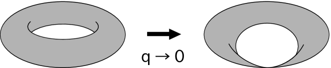
Figure 2: As $q\to 0$ one has a degenerate torus.

On the other hand, it is also known that $\widetilde{\Psi}_{\pm}^{(6\mathrm{vertex})}(s)$ by changing the variable to $S=\exp(i{\tilde{s}})$ becomes the Jack polynomial $J^{(\nu)}_{\lambda}(S)$ where $\lambda$ denotes the energy level. More precisely, by $\Delta=\left(\sin\tilde{s}\right)^{n+1}$ the Hamiltonian $H_{S}$ of the two-body Sutherland model is transformed into

$$H_{0}=\Delta^{-1}(H_{S}-e_{0})\Delta,~{}~{}~{}~{}~{}~{}H_{S}=-\frac{\partial^{2}}{\partial\tilde{s}^{2}}+\frac{n(n+1)}{\sin^{2}\tilde{s}},$$

whose eigenfunction is the Jack polynomial $J_{\lambda}^{(\nu)}(S)$. Here, $e_{0}$ stands for the eigenvalue of $H_{0}$ w.r.t. the ground-state $\Delta$. In addition, as $n\to 0$ $J^{(\nu)}_{\lambda}(S)$ reduces to the Schur function:

$$\chi_{\lambda}(S)=\frac{S^{1+\lambda}-S^{-1-\lambda}}{S-S^{-1}}.$$ (26)

Eq. (26) has its ${\mathfrak{sl}}_{N}$ analogy, i.e. given ${\bf S}={\rm diag}(S_{1},\cdots,S_{N})$ ($\det{\bf S}=1$) one has

$$\chi_{R}({\bf S})=\frac{\det(S_{i}^{R_{j}+N-j})}{\det(S_{i}^{N-j})},~{}~{}~{}~{}~{}~{}i,j=1,\cdots,N,$$

where $R=(R_{1},\cdots,R_{N-1},0)$ stands for a Young tableau. Each row length of $R$ obeys $R_{1}\geq R_{2}\geq\cdots$. In addition, there exists

$$(R_{1}-R_{2},\cdots,R_{i}-R_{i+1},\cdots,R_{N-1})=(\lambda_{1},\cdots,\lambda_{i},\cdots,\lambda_{N-1})$$

between $R$ and $\lambda\in P_{+}$ of ${\mathfrak{sl}}_{N}$.

To see the emergence of (26) on CFT side, we follow two steps below whose order differs from the above procedure.
${\bf Step~{}1}$: As mentioned in section 3, when the insertion becomes an identity operator ($\ell\to 0$) the toric conformal block reduces to the level-$k$ $\widehat{\mathfrak{sl}}_{2}$ character which is explicitly ($k\geq\lambda$, $\lambda$: highest weight)

$$\chi =\frac{\theta_{\sqrt{2}\lambda+1,k+2}-\theta_{-\sqrt{2}\lambda-1,k+2}}{\theta_{1,2}-\theta_{-1,2}},$$

$$\theta_{A,B} \equiv\theta_{A,B}(u_{1}|q^{\prime})=\sum_{n\in\mathbf{Z}+\frac{A}{2B}}(q^{\prime})^{Bn^{2}}\mathrm{e}^{2Bn\pi iu_{1}}.$$

${\bf Step~{}2}$: Next, we take $\tau^{\prime}\to i\infty$ such that only those terms involving ${\bf Z}=0$ inside the summation of $\theta_{A,B}$ survive. The above affine character $\chi$ factorizes into two parts depending on respectively $q^{\prime}$ and $u_{1}$:

$$\chi~{}\xrightarrow[q^{\prime}\to 0]{}~{}{q^{\prime}}^{\big{(}\frac{(\sqrt{2}\lambda+1)^{2}}{4\kappa}-\frac{1}{8}\big{)}}\frac{\mathrm{e}^{\pi i(\sqrt{2}\lambda+1)u_{1}}-\mathrm{e}^{-\pi i(\sqrt{2}\lambda+1)u_{1}}}{\mathrm{e}^{\pi iu_{1}}-\mathrm{e}^{-\pi iu_{1}}}.$$

Actually, the factor $\frac{(\sqrt{2}\lambda+1)^{2}}{4\kappa}-\frac{1}{8}$ comes from $L_{0}-\frac{c}{24}$. Because when the degeneration depicted in Fig. 2 occurs only the highest weight state in the integrable module $L_{k,\lambda}$ contributes to $\chi$. After dropping the $q^{\prime}$-dependent part we are simply left with ($\rho=1/\sqrt{2}$: Weyl vector)

$$\Psi~{}\xrightarrow[\ell\to 0]{}~{}\chi~{}\xrightarrow[q^{\prime}\to 0]{}~{}\frac{\mathrm{e}^{\pi i(\sqrt{2}\lambda+1)u_{1}}-\mathrm{e}^{-\pi i(\sqrt{2}\lambda+1)u_{1}}}{\mathrm{e}^{\pi iu_{1}}-\mathrm{e}^{-\pi iu_{1}}}=\frac{\mathrm{e}^{\pi i(\lambda+\rho)u}-\mathrm{e}^{-\pi i(\lambda+\rho)u}}{\mathrm{e}^{\pi i\rho u}-\mathrm{e}^{-\pi i\rho u}}.$$

This process we are studying then serves as a confirmation of the link (Table 1) between WZW model and the spin-1/2 XYZ chain.

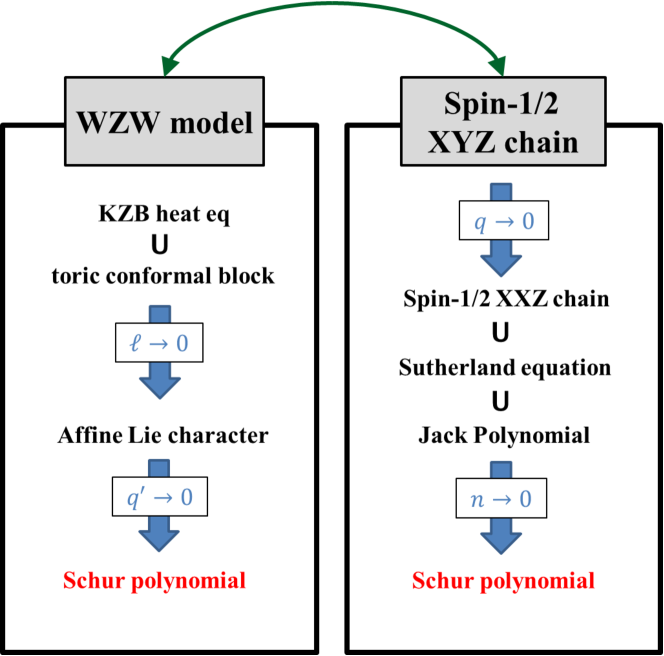
Figure 3: ${\bf(RHS)}$ A trigonometric degeneration of the spin-1/2 XYZ chain. ${\bf(LHS)}$ Through the identification $\ell/2=n$, toric conformal blocks reduce correspondingly to Schur polynomials (eigenstates of the two-body Sutherland model in RHS as $n\to 0$). Note that the order of two limits differs between RHS and LHS.

5 Summary

We have provided an interpretation of Stroganov’s “The Importance of being Odd” at the Razumov-Stroganov point by means of CFT language. We found that the total number of the XYZ chain sites $M=2n+1$ is equal to the dimension of the ${\mathfrak{sl}}_{2}$ representation space $V$ w.r.t. the primary field inserted on a torus in WZW model. Notice that $M$ must be odd. The approach summarized in Fig. 3 was used to support our proposal.

In fact, there is still another interesting limit mentioned in [16], i.e. $n\to\infty$ and $q\to 0$ with $t=8q^{\frac{3}{2}}n$ kept fixed as presented in Appendix. To study the corresponding deformation of WZW conformal blocks is an interesting future work, though the explicit form of them is not available. In the context of 2d Liouville field theory characterized by Virasora algebra, similar issues have been addressed in [33, 34].

Appendix

Under $n\to\infty$ and $q\to 0$ with $t=8q^{3/2}n$ kept fixed, one has $\Psi^{(8\text{vertex})}_{\pm}\to\mathcal{Q}_{\pm}(\theta,t)$.

By further adopting the new variable $\theta$ defined by $i\theta=s-\frac{1}{2}\pi\bar{\tau}$, this limit applied to (6) leads to a massive sine-Gordon model on a cylinder [16]:

$$t\frac{\partial}{\partial t}\mathcal{Q}_{\pm}(\theta,t)=\left\{\frac{\partial^{2}}{\partial\theta^{2}}-\frac{1}{8}t^{2}(\cosh 2\theta-1)\right\}\mathcal{Q}_{\pm}(\theta,t).$$

References

• [1] H.M. Babujian, “Off-shell Bethe Ansatz equation and N point correlators in SU(2) WZNW theory,” J. Phys. A26 (1993) 6981-6990 [hep-th/9307062].
• [2] H.M. Babujian and R. Flume, “Off-shell Bethe Ansatz equation for Gaudin magnets and solutions of Knizhnik-Zamolodchikov equations,” Mod. Phys. Lett. A9 (1994) 2029-2040 [hep-th/9310110].
• [3] B. Feigin, E. Frenkel and N. Reshetikhin, “Gaudin Model, Bethe Ansatz and Critical Level,” Comm. Math. Phys. 166 (1994) 27-62 [hep-th/9402022].
• [4] V. E. Korepin, N. M. Bogoliubov and A. G. Izergin, “Quantum Inverse Scattering Method and Correlation Functions,” Cambridge University Press, Cambridge (1993).
• [5] E. K. Sklyanin, “Quantum inverse scattering method. Selected topics,” (1991) in Quantum Groups and Quantum Integrable systems, Editor Mo-Lin Ge, Nankai Lectures in Mathematical Physics, World Scientific, Singapore, (1992) [hep-th/9211111].
• [6] V. G. Knizhnik and A. B. Zamolodchikov, “Current algebra and Wess-Zumino model in two dimensions,” Nucl. Phys. B247 (1984) 83-103.
• [7] G. Kuroki and T. Takebe, “Twisted Wess-Zumino-Witten models on elliptic curves,” Commun. Math. Phys.  190 (1997) 1 [q-alg/9612033].
• [8] H.M. Babujian, R. Poghossian and A. Lima-Santos, “Knizhnik- Zamolodchikov Bernard equations connected with eight vertex model,” Int. J. Mod. Phys. A14 (1999) 615-630 [solv-int/9804015].
• [9] G. Kuroki and T. Takebe, “Wess-Zumino-Witten model on elliptic curves at the critical level,” J. Phys. A34 (2001) 2403 [math/0005138 [math-qa]].
• [10] E. K. Sklyanin and , T. Takebe, “Algebraic Bethe Ansatz for XYZ Gaudin model,” Phys. Lett. A219 (1996) 217-225 [q-alg/9601028].
• [11] D. Bernard, “On the Wess-Zumino-Witten models on the torus,” Nucl. Phys. B303 (1988) 77-93.
• [12] P. I. Etingof and A. A. Kirillov, Jr., “Representations of affine Lie algebras, parabolic differential equations, and Lamé functions,” Duke Math. J. 74 (1994) 585-614 [hep-th/9310083].
• [13] T. Suzuki, “Differential equations associated to the SU(2) WZNW model on elliptic curves,” Publ. Res. Inst. Math. Sci. Kyoto 32 (1996) 207 [hep-th/9412219].
• [14] Y. G. Stroganov, “The Importance of being Odd,” J. Phys. A34 (2001) L179 [cond-mat/0012035].
• [15] A. V. Razumov and Y. G. Stroganov, “Spin chains and combinatorics,” J. Phys. A34 (2001) 3185 [cond-mat/0012141].
• [16] V. V. Bazhanov, V. V. Mangazeev, “Eight-vertex model and non-stationary Lamé equation,” J. Phys. A38 (2005) L145 [hep-th/0411094].
• [17] R. J. Baxter, “Partition function of the eight-vertex lattice model,” Ann. Phys. 70 (1972) 193.
• [18] R. Poghossian, “Deforming SW curve,” JHEP 1104 (2011) 033 [arXiv:1006.4822 [hep-th]].
• [19] F. Fucito, J. F. Morales, D. R. Pacifici and R. Poghossian, “Gauge theories on $\Omega$-backgrounds from non commutative Seiberg-Witten curves,” JHEP 1105 (2011) 098 [arXiv:1103.4495 [hep-th]].
• [20] Y. Zenkevich, “Nekrasov prepotential with fundamental matter from the quantum spin chain,” Phys. Lett. B701 (2011) 630-639 [arXiv:1103.4843 [math-ph]].
• [21] N. Dorey, S. Lee and T. J. Hollowood, “Quantization of Integrable Systems and a 2d/4d Duality,” JHEP 1110 (2011) 077 [arXiv:1103.5726 [hep-th]].
• [22] K. Muneyuki, T. -S. Tai, N. Yonezawa and R. Yoshioka, “Baxter’s T-Q equation, $SU(N)/SU(2)^{N-3}$ correspondence and $\Omega$-deformed Seiberg-Witten prepotential,” JHEP 1109 (2011) 125 [arXiv:1107.3756 [hep-th]].
• [23] N. A. Nekrasov, “Seiberg-Witten prepotential from instanton counting, ” Adv. Theor. Math. Phys.  7 (2004) 831 [hep-th/0206161]; N. Nekrasov and A. Okounkov, “Seiberg-Witten theory and random partitions,” hep-th/0306238.
• [24] R. J. Baxter, “Solving models in statistical mechanics,” Adv. Stud. Pure Math. 19 (1989) 95.
• [25] G. Felder and A. Varchenko, “Integral representation of solutions of the elliptic Knizhnik-Zamolodchikov-Bernard equations”, Int. Math. Res. notices N. 5 (1995) 221-233.
• [26] G. Felder, L. Stevens and A. Varchenko, “Modular transformations of the elliptic hypergeometric functions, Macdonald polynomials, and the shift operator,” Moscow Mathematical Journal 3 (2003) 457 [math/0203049].
• [27] T. -S. Tai, “Triality in SU(2) Seiberg-Witten theory and Gauss hypergeometric function,” Phys. Rev. D82 (2010) 105007 [arXiv:1006.0471 [hep-th]].
• [28] T. -S. Tai, “Uniformization, Calogero-Moser/Heun duality and Sutherland/bubbling pants,” JHEP 1010 (2010) 107 [arXiv:1008.4332 [hep-th]].
• [29] N. A. Nekrasov and S. L. Shatashvili, “Quantum integrability and supersymmetric vacua,” Prog. Theor. Phys. Suppl.  177 (2009) 105 [arXiv:0901.4748 [hep-th]].
• [30] L. F. Alday, D. Gaiotto and Y. Tachikawa, “Liouville Correlation Functions from Four-dimensional Gauge Theories,” Lett. Math. Phys.  91 (2010) 167 [arXiv:0906.3219 [hep-th]].
• [31] N. A. Nekrasov and S. L. Shatashvili, “Quantization of Integrable Systems and Four Dimensional Gauge Theories,” arXiv:0908.4052 [hep-th].
• [32] N. Nekrasov, A. Rosly and S. Shatashvili, “Darboux coordinates, Yang-Yang functional, and gauge theory,” Nucl. Phys. Proc. Suppl.  216 (2011) 69 [arXiv:1103.3919 [hep-th]].
• [33] A. Mironov and A. Morozov, “Nekrasov Functions and Exact Bohr-Zommerfeld Integrals,” JHEP 1004 (2010) 040 [arXiv:0910.5670 [hep-th]].
• [34] V. Alba and A. Morozov, “Non-conformal limit of AGT relation from the 1-point torus conformal block,” JETP Lett.  90 (2009) 708 [arXiv:0911.0363 [hep-th]].