Phase Separation with Anisotropic Coherency Strain

Abstract

We consider the effects of anisotropic coherency strain (due to lattice mismatch) on phase separation in intercalation materials, motivated by the high-rate Li-ion battery material Li_xFePO₄. Using a phase-field model coupled to elastic stresses, we analyze spinodal decomposition (linear instability of the homogeneous state) as well as nonlinear evolution of the phase pattern at constant mean filling. We consider fully anisotropic coherency strain and focus on the case of simultaneous expansion and contraction along different crystal axes, as in the case of Li_xFePO₄, which leads to tilted, striped phase boundaries in equilibrium.

1 Introduction

Intercalation, i.e. the reversible insertion of molecules in a host solid, is a general phenomenon with many applications in chemical physics. Of particular interest today is the intercalation of lithium ions in the active solid particles of Li-ion battery composite electrodes. Li-ion batteries have become essential for portable electronic devices such as cell phones and power tools and are advancing toward possible use in electric vehicles or renewable energy storage, due to higher energy density and power density than earlier battery chemistries [1, 2, 3]. In particular, Li_xFePO₄  has gained considerable attention as a leading cathode material candidate because of its high power density, fast charging times, long cycle life, and favorable safety characteristics [4, 5, 6].

Modeling ion intercalation dynamics in crystalline particles is a complex problem at the intersection of physics, chemistry, materials science, and applied mathematics [7, 8, 9]. A standard assumption in Li-ion battery models is that diffusion is linear and isotropic within the solid [7, 10], but it is becoming recognized that this is often not the case, due to the anisotropic crystalline nature of most solid hosts. In particular, experiments and ab initio computer simulations have revealed that Li diffusion in Li_xFePO₄  is highly anisotropic and exhibits a strong tendency for phase-separation between lithiated (LiFePO₄) and delithiated (FePO₄) states [11, 12, 13]. Additionally, this FePO₄/LiFePO₄ phase boundary tends to reach the active (010) surface and align itself along {101} or {100} crystal planes [11, 15, 13], which suggests an intimate connection between phase separation dynamics and the elastic properties of the crystal. In contrast, motivated by the first experimental paper [4], existing battery engineering models for Li_xFePO₄assume a spherical “shrinking core” of one phase being replaced by a shell of the other [16, 17] and thus do not model phase separation dynamics, anisotropic diffusion or coherency strain.

Over the past five years, our group has developed a general phase-field model for intercalation kinetics in nanoparticles, which is helping to unravel the complex dynamical behavior of Li_xFePO₄and interpret experimental data from microscopic first principles  [18, 19, 20, 21, 22, 23, 24]. A crucial contribution of this work has been to consistently formulate the kinetics of electrochemical charge-transfer reactions at the surface of the active particles with the non-equilibrium thermodynamics of bulk ion transport and phase separation via a modified Butler-Volmer theory for concentrated solutions and solids [18, 24]. This has led to novel predictions for intercalation dynamics in nano particles, such as size-dependent miscibility and spinodal gaps [21, 25], ion intercalation waves filling the crystal layer by layer (rather than shrinking core) at low currents [19, 20, 26], and quasi-solution behavior and suppressed phase separation at high currents [22, 23].

In this work, we focus on understanding the general effects of coherency strain on bulk phase separation, while neglecting the coupling to electrochemical reactions. (For a complete model of Li_xFePO₄nanoparticles under applied current, see Ref. [23].) Classical phase-field models in materials science have included effects of elastic coherency strain for isotropic solids [41, 42, 34, 35], but here we analyze phase separation with anisotropic coherency strain, focusing on the novel case where both contraction and expansion occur along different crystal planes, as in Li_xFePO₄. Simplified elastic models of Li_xFePO₄have led to the conclusion that phase separation occurs along the {100} crystal planes [36, 37, 26], as in some experiments [15], even though {101} phase boundaries are also sometimes observed [11, 13]. Here we show that such tilted phase boundaries result from simultaneous contraction and expansion in different directions. To address dynamical behavior, we perform a linear stability analysis on the model to predict parameter regimes for spinodal decomposition of the system, which provides analytical predictions for initial instabilities in the concentration and deformation fields. As the nonuniform states are highly nonlinear, numerical simulations are necessary to examine the long-term behavior of phase-separated solutions.

2 Model Formulation

To develop a phase-field model of this system, we begin by defining an order parameter $c$ to be the dimensionless, normalized concentration of Li, where $c=1$ corresponds to an entirely lithiated phase (LiFePO₄), and $c=0$ to an entirely delithiated one (FePO₄). The total free energy of the system described by the domain $\Omega$ can be expressed as a functional of the local Li concentration in the Cahn-Hilliard formulation

$$\mathscr{F}[c]=\int_{\Omega}\left\{f(c)+\frac{\rho}{2}\nabla c\cdot({\bf K}\nabla c)+\frac{1}{2}{\bf E}:{\bf T}\right\}\text{d}{\bf x},\quad{\bf x}\in\Omega,$$ (1)

where $f(c)$ is the free energy density of a homogeneous state, $\rho$ is the number density of intercalation sites, and the gradient term (with ${\bf K}$ being a symmetric, positive definite tensor) is the next order term in an expansion about this state which penalizes spatial phase modulation in the system [27, 28]. For our model, we take this tensor to be constant. Li insertion into this material has been observed to produce significant anisotropic strains which range from about -2% to 5% to maintain coherency between states [36], and hence we also take into account long-range elastic contributions to the free energy as in previous phase-field models [34, 35]. The elastic energy is represented in the final term of the integrand in Equation (1) with the contraction between the tensors ${\bf E}$ and ${\bf T}$, which are the strain and stress tensors respectively. To capture the effects of the interactions between lithiated and delithiated states, we take the regular solution model for the homogeneous energy density [27]

$$f(c)=a\rho c(1-c)+\rho k_{B}T\left[c\log(c)+(1-c)\log(1-c)\right],$$ (2)

where $k_{B}$ is the Boltzmann constant, $T$ is the absolute temperature, and the regular solution interaction parameter $a$ is the average energy density of ion intercalation. The first term in Equation (2) is the enthalpic contribution which favors phase separation, while the second term is the entropic contribution which promotes phase mixing. The elements of the adjusted infinitesimal strain tensor are given by the kinematic relationship

$${\bf E}=\frac{1}{2}\left(\nabla{\bf u}+\nabla{\bf u}^{\text{T}}\right)-c{\bf M},$$ (3)

where ${\bf u}$ is the deformation vector, and ${\bf M}$ is the lattice mismatch tensor of the lithiated and unlithiated phases. This additional mismatch term is the stress-free strain when the density is $c$. Noting that the intercalation of these particles takes the delithiated orthorhombic crystal (FePO₄) to another orthorhombic state (LiFePO₄), insertion will hence only induce compressions and expansions of the surrounding material. Consequently, the tensor ${\bf M}$ will be diagonal. Assuming the strains to be within the regime of linear elasticity, we can then use Hooke’s law to describe the stress in terms of the constitutive equation

$${\bf T}={\bf C}:{\bf E},$$ (4)

where ${\bf C}$ is the rank-4 elasticity tensor [38], which for orthorhombic crystals, can be described by nine distinct elements [33]. We now use this free energy to calculate the chemical potential as

$$\mu\equiv\frac{1}{\rho}\frac{\delta\mathscr{F}}{\delta c}=\frac{1}{\rho}\frac{\partial}{\partial c}\left[f(c)+\frac{1}{2}{\bf E}:{\bf T}\right]-\nabla\cdot({\bf K}\nabla c),$$ (5)

where

$$\frac{\partial f}{\partial c}=\,a\rho(1-2c)+\rho k_{B}T\log\left(\frac{c}{1-c}\right),\quad\frac{1}{2}\frac{\partial}{\partial c}\left({\bf E}:{\bf T}\right)=-{\bf M}:{\bf T}.$$ (6)

Note that as ${\bf M}$ is diagonal, only the compressional components of the stress will affect the chemical potential. The mass flux is then expressed as

$${\bf j}=-\rho c{\bf B}\nabla\mu,$$ (7)

where ${\bf B}$ is the mobility tensor. Strictly speaking, the mobility must depend on concentration, e.g. as ${\bf B}\sim(1-c)$ in the classical Cahn-Hilliard regular solution model [28], but below we will make simpler assumptions that have relatively little effect on the dynamics of coherency phase separation.

Finally, the evolution of the concentration field is calculated with a conservation law within the cathode

$$\rho\frac{\partial c}{\partial t}+\nabla\cdot{\bf j}=0,$$ (8)

and at any given time, a quasi-steady approximation of mechanical equilibrium is given by

$$\nabla\cdot{\bf T}={\bf 0}.$$ (9)

Using Equations (3), (4) and (9), we can write this elastostatic condition in terms of the deformation field components as the system

$$\frac{\partial}{\partial x}\sum_{k=1}^{3}C_{1k}\frac{\partial u_{k}}{\partial x_{k}}+C_{66}\frac{\partial}{\partial y}\left(\frac{\partial u_{1}}{\partial y}+\frac{\partial u_{2}}{\partial x}\right)+C_{55}\frac{\partial}{\partial z}\left(\frac{\partial u_{3}}{\partial x}+\frac{\partial u_{1}}{\partial z}\right)=\sum_{k=1}^{3}C_{1k}M_{kk}\frac{\partial c}{\partial x},$$ (10a)

$$\frac{\partial}{\partial y}\sum_{k=1}^{3}C_{2k}\frac{\partial u_{k}}{\partial x_{k}}+C_{44}\frac{\partial}{\partial z}\left(\frac{\partial u_{2}}{\partial z}+\frac{\partial u_{3}}{\partial y}\right)+C_{66}\frac{\partial}{\partial x}\left(\frac{\partial u_{1}}{\partial y}+\frac{\partial u_{2}}{\partial x}\right)=\sum_{k=1}^{3}C_{2k}M_{kk}\frac{\partial c}{\partial y},$$ (10b)

$$\frac{\partial}{\partial z}\sum_{k=1}^{3}C_{3k}\frac{\partial u_{k}}{\partial x_{k}}+C_{55}\frac{\partial}{\partial x}\left(\frac{\partial u_{3}}{\partial x}+\frac{\partial u_{1}}{\partial z}\right)+C_{44}\frac{\partial}{\partial y}\left(\frac{\partial u_{2}}{\partial z}+\frac{\partial u_{3}}{\partial y}\right)=\sum_{k=1}^{3}C_{3k}M_{kk}\frac{\partial c}{\partial z},$$ (10c)

where we are using the standard convention to reduce the elasticity tensor elements $C_{ijkl}$ to the matrix components $C_{ij}$ [39]. This hence gives the elastic energy contribution to the chemical potential

$$\frac{1}{2}\frac{\partial}{\partial c}\left({\bf E}:{\bf T}\right)=-{\bf M}:{\bf T}=\sum_{i=1}^{3}\left[\sum_{j=1}^{3}C_{ij}M_{jj}\left(M_{ii}c-\frac{\partial u_{i}}{\partial x_{i}}\right)\right].$$ (11)

With the bulk equations established for Li migration within the cathode, boundary conditions must be formulated at the electrode-electrolyte interfaces to close the model. Mass balance at the interface must satisfy

$${\bf n}\cdot{\bf j}+R(c,\mu)=0,$$ (12)

where ${\bf n}$ is the outward normal to the surface, and $R(c,\mu)$ is the potential-dependent interfacial reaction rate [18, 21, 22, 23, 24]. We additionally assume the so-called variational boundary condition

$${\bf n}\cdot({\bf K}\nabla c)=0,$$ (13)

which is reasonable for our system in which concentration gradients are observed to be perpendicular to the particle surface [burch09]. Finally, we assume a uniform pressure field of strength $P$ from the surrounding matrix, which gives the interfacial stress balance

$${\bf n}\cdot({\bf T}+P{\bf I})={\bf 0}.$$ (14)

It should be noted that we state the boundary conditions above just to show the form of the complete model, but we will not use them in our calculations below. As the particular focus of this work is a feature of the bulk dynamics, we take the infinite domain $\Omega=\mathbb{R}^{3}$, and hence only boundedness in the far-field of the concentration and deformation fields is necessary for the purposes of our analysis. Detailed studies of current dependence and finite size effects for ion intercalation in nanoparticles can be found in [22, 23, 21, 25, 26, 40].

3 Isotropic Coherency Strain

To begin to understand the leading order effects of lithiation induced strains in Li_xFePO₄, we start by taking the host material to be an isotropic body. Under this assumption, the coefficients of the elasticity tensor reduce to

$$C_{11}=C_{22}=C_{33}=2\left(\frac{1-\nu}{1-2\nu}\right)G,\quad C_{44}=C_{55}=C_{66}=G,$$ (15)

$$C_{12}=C_{21}=C_{23}=C_{32}=C_{13}=C_{31}=\left(\frac{2\nu}{1-2\nu}\right)G,$$ (16)

where $G$ is the shear modulus, and $\nu$ is the Poisson ratio. We further take the coherency strains to be isotropic, which simplifies the mismatch tensor to the form ${\bf M}=M_{\text{iso}}{\bf I}$, where $M_{\text{iso}}$ is a scalar. We can then write the elastostatic condition (9) in terms of the deformation vector as

$$(1-2\nu)\nabla^{2}{\bf u}+\nabla(\nabla\cdot{\bf u})=2M_{\text{iso}}(1+\nu)\nabla c.$$ (17)

Note that this also simplifies the elastic contribution to the chemical potential to

$$\frac{1}{2}\frac{\partial}{\partial c}\left({\bf E}:{\bf T}\right)=-M_{\text{iso}}\text{tr}\{{\bf T}\}=2M_{\text{iso}}G\left(\frac{1+\nu}{1-2\nu}\right)\left[3M_{\text{iso}}c-\nabla\cdot{\bf u}\right].$$ (18)

If we take the curl of Equation (17), we obtain $\nabla^{2}(\nabla\times{\bf u})=0$. From potential theory, we know that ${\bf u}$ must then be curl free and can be written in terms of the gradient of a scalar potential: ${\bf u}=\nabla\psi$. This gives the equation

$$\nabla\left[\nabla^{2}\psi-M_{\text{iso}}\left(\frac{1+\nu}{1-\nu}\right)c\right]={\bf 0}.$$ (19)

This can then be integrated with the constant of integration taken as zero without loss of generality. We hence have the dilatation, $\nabla\cdot{{\bf u}}$, as

$$\nabla\cdot{{\bf u}}=\nabla^{2}\psi=M_{\text{iso}}\left(\frac{1+\nu}{1-\nu}\right)c$$ (20)

and can use this to rescale the enthalpic contribution in the chemical potential as

$$\mu=a-2bc+k_{B}T\log\left(\frac{c}{1-c}\right)-\nabla\cdot({\bf K}\nabla c),\quad b=a-2M_{\text{iso}}^{2}\left(\frac{1+\nu}{1-\nu}\right)\frac{G}{\rho}.$$ (21)

Note that this result was first obtained and analyzed for phase-field models in [41, 42].

We can next obtain a spinodal region in the parameter space, which is the region in which homogeneous concentrations are linearly unstable. The homogeneous state of the system can be calculated by taking $c=c_{0}$ to be constant, and in perturbing this state with the infinitesimal quantity $\tilde{c}=c-c_{0}$, the linearized evolution equation for the concentration perturbation will take the form

$$\frac{\partial\tilde{c}}{\partial t}=c_{0}\nabla\cdot\left\{{\bf B}\nabla\left[\left(-2b+\frac{k_{B}T}{c_{0}(1-c_{0})}\right)\tilde{c}-\nabla\cdot({\bf K}\nabla\tilde{c})\right]\right\}.$$ (22)

By assuming the normal mode of the perturbation as $\tilde{c}=\hat{c}\exp(\sigma t+i{\bf q}\cdot{\bf x})$, where $\sigma$ is growth rate of a given wave vector ${\bf q}$, this gives the dispersion relation

$$\sigma({\bf q})=-c_{0}{\bf q}\cdot({\bf B}{\bf q})\left[-2b+\frac{k_{B}T}{c_{0}(1-c_{0})}+{\bf q}\cdot({\bf K}{\bf q})\right].$$ (23)

The spinodal can now be calculated for parameters in which there exists a positive growth rate, and hence we have the region defined by

$$M_{\text{iso}}^{2}<\frac{\rho}{4G}\left(\frac{1-\nu}{1+\nu}\right)\left[2a-\frac{k_{B}T}{c_{0}(1-c_{0})}\right].$$ (24)

It is important to note that this stability criterion is independent of the sign of $M_{\text{iso}}$, and hence both crystal expansion and contraction will have the same effect. Additionally, the increase of elastic strains narrows the stability region in parameter space and can even annihilate the spinodal for a given interaction parameter $a$ as shown in Figure (1). The parameters obtained from experiment are listed in the caption. This latter point is somewhat troubling as not only does Li_xFePO₄ exhibit both high strains and phase-separation upon intercalation, but the phase-separation in this material has been observed to occur along the direction of greatest strain [15, 44]. This apparent contradiction is resolved in the following section.

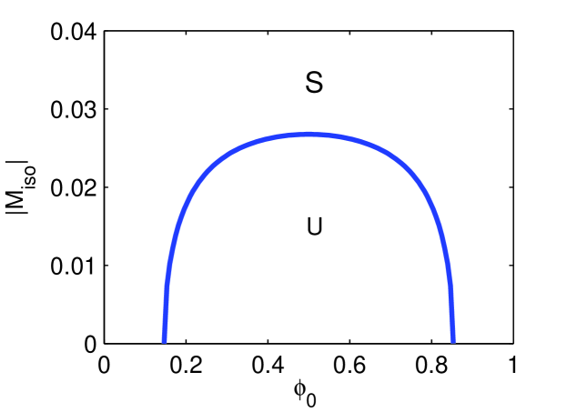
Figure 1: Spinodal region in terms of the isotropic lattice mismatch $M_{\text{iso}}$ and homogeneous concentration $c_{0}$. The stable and unstable regions are labeled within the figure. The parameters used are $a=1.6\times 10^{-20}\,\text{J}$ [43], $\rho=14\,\text{nm}^{-3}$, $G=5\times 10^{10}\,\text{Pa}$, $\nu=0.22$ [33], and $k_{B}T=4\times 10^{-21}\,\text{J}$ at room temperature.

4 Anisotropic Coherency Strain

To account for the alignment of the FePO₄/LiFePO₄ phase boundary with the $(b,c)$ plane of the host crystal, we must include anisotropic properties of the system into our model (note that we are using the standard notation for the axis labels of Li_xFePO₄ as seen in [15]). In particular, a more appropriate approximation for the mismatch tensor corresponding to this system would be diagonal with distinct values. For Li_xFePO₄, these diagonal elements are roughly: $M_{11}=0.052$, $M_{22}=0.036$ and $M_{33}=-0.019$ [15]. To capture the effects of anisotropic coherency strains, we will simplify the model by reducing the remaining tensors to scalars as ${\bf B}=B{\bf I}$ and ${\bf K}=K{\bf I}$, as they merely act as spatial scalings. We can then easily nondimensionalize the spatial and temporal coordinates with the following relations

$${\bf x}\rightarrow\lambda{\bf x},\quad t\rightarrow\frac{\lambda^{2}}{\mathcal{D}}t,\quad\lambda=\sqrt{\frac{K}{k_{B}T}}.$$ (25)

where we have used the Einstein mobility relation to introduce the diffusivity $\mathcal{D}=k_{B}TB$. The characteristic length-scale, $\lambda$, represents the typical width of the FePO₄/LiFePO₄ interface which is on the order of nanometers [15]. We hence obtain the concentration evolution

$$\frac{\partial c}{\partial t}=\nabla\cdot\left\{c\nabla\left[-2\alpha c+\log\left(\frac{c}{1-c}\right)-\nabla^{2}c-\frac{1}{\rho k_{B}T}\sum_{i=1}^{3}\sum_{j=1}^{3}M_{ii}C_{ij}\frac{\partial u_{j}}{\partial x_{j}}\right]\right\},$$ (26)

$$\text{where}\quad\alpha=\frac{a}{k_{B}T}-\frac{1}{2\rho k_{B}T}\sum_{i=1}^{3}\sum_{j=1}^{3}M_{ii}C_{ij}M_{jj},$$ (27)

which is coupled with the equilibrium conditions (10). To further further illuminate the effects of coherency strain anisotropy, we again take the host material to be an isotropic body. While this is not quite physical, simulations have been performed for both isotropic and anisotropic bodies using the elastic moduli found in [33] to verify this approximation, and no qualitative differences have been observed. Furthermore, as also seen in [33], the anisotropy is much stronger in the lattice mismatch (e.g. a contraction along the $c$-axis is induced by insertion), and hence these effects are amplified by the fact that while the energetic contributions from elasticity are $\mathcal{O}(C_{ij})$, they are indeed quadratic in the mismatch parameters [45]. This system therefore simplifies to

$$\frac{\partial c}{\partial t}=\nabla\cdot\left\{c\nabla\left[-2\alpha c+\log\left(\frac{c}{1-c}\right)-\nabla^{2}c-2\gamma\left({\bf M}\nabla+\frac{\nu}{1-2\nu}\text{tr}\{{\bf M}\}\nabla\right)\cdot{\bf u}\right]\right\},$$ (28)

$$(1-2\nu)\nabla^{2}{\bf u}+\nabla(\nabla\cdot{\bf u})=2\left[(1-2\nu){\bf M}\nabla+\nu\,\text{tr}\{{\bf M}\}\nabla\right]c,$$ (29)

$$\text{where}\quad\alpha=\frac{a}{k_{B}T}-\gamma\left[\text{tr}\{{\bf M}^{2}\}+\left(\frac{\nu}{1-2\nu}\right)\text{tr}\{{\bf M}\}^{2}\right],\quad\gamma=\frac{G}{\rho k_{B}T},$$ (30)

and tr{$\circ$} denotes the trace operator. As before, we perturb our system about the basic state of constant concentration and zero deformations to obtain the linearized system

$$\frac{\partial\tilde{c}}{\partial t}=c_{0}\nabla^{2}\left[\left(-2\alpha+\frac{1}{c_{0}(1-c_{0})}\right)\tilde{c}-\nabla^{2}\tilde{c}-2\gamma\left({\bf M}\nabla+\frac{\nu}{1-2\nu}\text{tr}\{{\bf M}\}\nabla\right)\cdot\tilde{{\bf u}}\right],$$ (31)

$$(1-2\nu)\nabla^{2}\tilde{{\bf u}}+\nabla(\nabla\cdot\tilde{{\bf u}})=2\left[(1-2\nu){\bf M}\nabla+\nu\,\text{tr}\{{\bf M}\}\nabla\right]\tilde{c}.$$ (32)

By introducing the vector of fields $\tilde{\bf v}=(\tilde{u}_{1},\tilde{u}_{2},\tilde{u}_{3},\tilde{c})$, we can again take the normal mode of the perturbations as $\tilde{\bf v}=\hat{\bf v}\exp(\sigma t+i{\bf q}\cdot{\bf x})$ and obtain a linear algebraic system of the form ${\bf\Lambda}\hat{\bf v}={\bf 0}$. This operator can then be written as ${\bf\Lambda}(\sigma,{\bf q})={\bf\Sigma}(\sigma)+{\bf Q}({\bf q})$, where $\Sigma_{44}=\sigma$ is the only nonzero element of ${\bf\Sigma}$, and the elements of ${\bf Q}$ are given in the Appendix. For the perturbation eigenvector $\hat{\bf v}$ to have nontrivial solutions, the operator ${\bf\Lambda}$ must be singular (i.e. $\text{det}\{{\bf\Lambda}\}=0$), and hence we obtain the dispersion relation for the growth rate of a given spatial mode

$$\sigma({\bf q})=\frac{-\text{det}\{{\bf Q}({\bf q})\}}{\text{det}\{{\bf Q}^{(4)}({\bf q})\}},$$ (33)

where the parenthetical superscript denotes the submatrix of ${\bf Q}$ obtained by removing the fourth row and column. A typical plot of $\sigma$ can be seen in Figure (2). For presentation purposes, we have only shown a slice in the $(x,y)$ plane. Lighter colors denote larger growth rates, the curve represents the zero (neutral) contour of $\sigma$, and the $\times$’s mark the points of greatest growth. The parameters are the same as those used in Figure (1) with the addition of lattice mismatch rates listed in the caption obtained by [15]. Note that the most excited wave-vectors lie along the $x$-axis, which for the parameters used, is the direction of greatest strain. To further understand this, we take the simple case of unidirectional strain ($M_{11}=M_{\text{uni}}$, $M_{22}=M_{33}=0$). If we then write the growth rate as $\sigma({\bf q})=\sigma_{0}({\bf q})+\sigma_{s}({\bf q})$, where $\sigma_{0}$ is the growth in the absence of strain (i.e. $M_{\text{uni}}\rightarrow 0$), and $\sigma_{s}$ is the strain induced contribution, then this contribution takes the form

$$\sigma_{s}({\bf q})=-\frac{2\gamma c_{0}M_{\text{uni}}^{2}}{(1-\nu)q^{2}}\left(q_{y}^{2}+q_{z}^{2}\right)^{2},\quad q=|{\bf q}|.$$ (34)

It can be seen here that this contribution is minimized for a given wave vector of magnitude $q$ in the $(q_{y},q_{z})$ plane, which means that phase-separation is suppressed the most in directions orthogonal to the unidirectional strain. Additionally, along the vector ${\bf q}=(q_{x},0,0)$, the strain induced contribution is maximized at $\sigma_{s}=0$, which means that the direction of strain for this case is the only direction without suppression. It can be shown that if all $M_{ii}$ have the same sign (i.e. pure expansions or pure contractions), then phase-separation will always occur in the direction in which $|M_{ii}|>|M_{jj}|,|M_{kk}|$ (i.e. the direction of largest strain), however it will be seen in the next section that the presence both contractions and expansions result in the possibility of skewed phase interfaces.

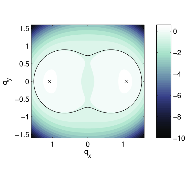
Figure 2: Dispersion relation with anisotropic mismatch strains. The curve indicates neutral stability (i.e. $\sigma=0$), while the $\times$’s mark the largest growth rates. The lattice mismatch parameters used are $M_{11}=0.052$, $M_{22}=0.036$ and $M_{33}=-0.019$ [33].

5 Numerical Simulations

To verify the results from the linear stability analysis, we perform numerical simulations of the governing equations (28-29), as this analysis can only predict the initial dynamics still within the linear regime. Both two- and three-dimensional simulations are presented to represent two limits of this system.

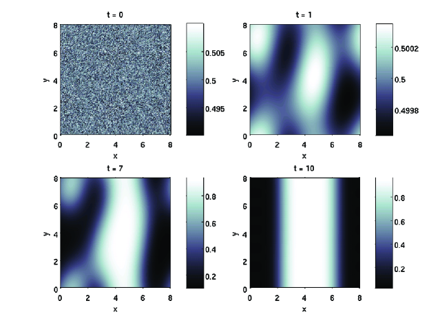
Figure 3: Time evolution of system (28-29) starting from the state $c=0.5$ perturbed with small amplitude noise at $t=0,1,7,10$ as labeled.

5.1 Phase Separation with Anisotropic Plane Strain

We first present the limit in which strains along the $c$-axis are neglected (i.e. $u_{3}\rightarrow 0$) under the assumption that Li transport along molecular channels direction is in constant equilibrium due to the very fast mobility [12] and suppressed phase separation [23]. This is a reasonable assumption for reaction-limited Li_xFePO₄nano particles [19, 22], but would break down in larger particles ($>100$nm) due to channel-blocking Li/Fe anti-site defects, which lead to size-dependent effective mobility [14]. Note that the stability results from section (4) remain unchanged for the two-dimensional case. For numerical convenience, we will further approximate the flux (before the rescaling) as ${\bf j}=-B\nabla\mu$. This is a common assumption in phase-field modeling since the prefactor $c$ merely scales the initial time evolution and does not affect long-term behavior of the system which is solely determined by the form of the chemical potential [30, 35, 41]. We use a pseudo-spectral method for the spatial differentiation with $256\times 256$ modes and a semi-implicit scheme for temporal updating. The linear terms are handled with the backward Euler method, which although only first order accurate in time, provides the necessary stability required for the stiff solutions of the system. The second order Adams-Bashforth method is used for the nonlinearities, and periodic boundary conditions are used to approximate the infinite domain. As the equations for the deformation fields are linear, they can be solved exactly in Fourier space in terms of the order parameter, and hence the system can be reduced to a single evolution equation. If we define the Fourier transform of the order parameter as $\mathfrak{F}\{c({\bf x},t)\}\equiv\phi({\bf q},t)$, where ${\bf q}$ is the corresponding wave-vector, the evolution of $\phi$ in Fourier space will be therefore governed by

$$\frac{d\phi}{dt}=\; \left(2\alpha q^{2}-q^{4}+\frac{\gamma\mathcal{M}({\bf q})}{(1-\nu)(1-2\nu)q^{2}}\right)\phi-q^{2}\mathfrak{F}\left\{\log\left(\frac{c}{1-c}\right)\right\},$$ (35)

where the contribution from the coherency strains is given as

$$\mathcal{M}({\bf q})=\; \left[(1-\nu)M_{11}+\nu M_{22}\right]\left[\left((1-\nu)q^{2}+q_{y}^{2}\right)M_{11}+\left(\nu q^{2}-q_{y}^{2}\right)M_{22}\right]q_{x}^{2}$$ (36)

$$+\left[\nu M_{11}+(1-\nu)M_{22}\right]\left[\left(\nu q^{2}-q_{x}^{2}\right)M_{11}+\left((1-\nu)q^{2}+q_{x}^{2}\right)M_{22}\right]q_{y}^{2}.$$ (37)

A typical simulation evolved from the state $c=0.5$ perturbed with small amplitude noise is shown at various times in Figure (3). These perturbations are initially damped, and regions of localized concentrations begin to form. The regions coarsen until the concentration is aligned with the $y$-axis confirming the spontaneous phase-separation along the direction of greatest strain. Note that the parameters are the same as those listed in the captions of Figures (1) and (2) excluding contributions from the third dimension. It should be mentioned that this model is quite robust, as similar results can be obtained from simulations over a wide range of parameters.

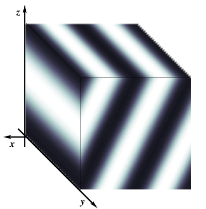
Figure 4: Equilibrium state of Li_xFePO₄with anisotropic coherency strain in three dimensions showing skewed, striped phases.

5.2 Three Dimensional Coherency Strain in Li_xFePO₄

For a more complete picture of phase separation in Li_xFePO₄, it is necessary to consider fully anisotropic three-dimensional coherency strain. In particular, we perform full three-dimensional simulations to include the effects of contractions in the $c$-direction. As seen in Figure (4), the equilibrium state results in skewed interfaces, which have also been seen in some experiments [11, 13].

6 Conclusions

We have considered the intercalation of Li within Li_xFePO₄ as a model system which exhibits both phase-separation and highly anisotropic coherency strains. A phase-field model which incorporates energetic contributions from entropy, enthalpy and elastic properties of the host material has been developed. We have shown through linear stability analysis that while coherency strains suppress phase-separation, this suppression is maximized in directions orthogonal to the direction of a given strain. Hence the system is expected to phase-separate along the direction of greatest strain ($a$-axis) given sufficiently large enthalpic contributions. As linear stability theory can only predict the initial evolution of spinodal decomposition, numerical simulations were performed on an idealized system to illuminate the effects of coherency strain anisotropy, and phase boundaries were observed to align perpendicularly to the $a$-axis as observed in experiment. Coherency strain anisotropy has therefore been shown to be a possible mechanism for this alignment. We have also considered phase separation in the three dimensional case with fully anisotropic coherency strain, including contraction along the $c$ axis. This leads to skewed phase boundaries, which have also been seen in some experiments. These interesting observations are unified and extended to electrochemically driven intercalation at fixed current in Ref. [23].

Appendix

The elements of ${\bf Q}$ are listed as follows, where we have defined $q\equiv|{\bf q}|$ with ${\bf q}=(q_{x},q_{y},q_{z})$.

$$Q_{11}=(1-2\nu)q^{2}+q_{x}^{2},\quad Q_{12}=q_{x}q_{y},\quad Q_{13}=q_{x}q_{z},\quad Q_{14}=2i[(1-2\nu)M_{11}+\nu M_{kk}]q_{x},$$

$$Q_{21}=q_{y}q_{x},\quad Q_{22}=(1-2\nu)q^{2}+q_{y}^{2},\quad Q_{23}=q_{y}q_{z},\quad Q_{24}=2i[(1-2\nu)M_{22}+\nu M_{kk}]q_{y},$$

$$Q_{31}=q_{z}q_{x},\quad Q_{32}=q_{z}q_{y},\quad Q_{33}=(1-2\nu)q^{2}+q_{z}^{2},\quad Q_{34}=2i[(1-2\nu)M_{33}+\nu M_{kk}]q_{z},$$

$$Q_{41}=-2i\gamma c_{0}\left(M_{11}+\frac{\nu M_{kk}}{1-2\nu}\right)q^{2}q_{x},\quad Q_{42}=-2i\gamma c_{0}\left(M_{22}+\frac{\nu M_{kk}}{1-2\nu}\right)q^{2}q_{y},$$

$$Q_{43}=-2i\gamma c_{0}\left(M_{33}+\frac{\nu M_{kk}}{1-2\nu}\right)q^{2}q_{z},\quad Q_{44}=-c_{0}\left(2\alpha-\frac{1}{c_{0}(1-c_{0})}-q^{2}\right)q^{2}.$$

References

- [1] S. Megahed and B. Scrosati, Lithium-ion rechargeable batteries, J. Power Sources 51, 79 (1994).
- [2] M. Wakihara and O. Yamamoto (eds.), Lithium Ion Batteries (Kodansha & Wiley-VCH, Wenheim, 1998).
- [3] B. Scrosati, Recent advances in lithium ion battery materials, Electrochimica Acta 45, 2461 (2000).
- [4] A.K. Padhi, K.S. Nanjundaswamy and J.B. Goodenough, Phospho-olivines as positive-electrode materials for rechargeable lithium batteries, J. Electrochem. Soc. 144 1188 (1997).
- [5] J.-M. Tarascon and M. Armand, Issues and challenges facing rechargeable lithium battery cathodes, Nature 414, 359 (2001).
- [6] B. Kang and G. Ceder, Battery materials for ultrafast charging and discharging, Nature 458, 190 (2009).
- [7] J. Newman, Electroochemical Systems (Prentice-Hall, Inc., Englewood Cliffs, NJ, 2nd ed., 1991).
- [8] A. J. Bard and L. R. Faulkner, Electrochemical Methods (John Wiley & Sons, Inc., New York, NY, 2001).
- [9] I. Rubinstein, Electro-Diffusion of Ions (SIAM Studies in Applied Mathematics, SIAM, Philadelphia, PA, 1990).
- [10] M. Doyle, T. F. Fuller and J. Newman, Modeling of galvonistic charge and discharge of the lithium/polymer/insertion cell, J. Electrochem. Soc. 140, 1526 (1993).
- [11] L. Laffont, C. Delacort, P. Gibot, M. Y. Wu, P. Kooyman, C. Masquelier and J. M. Tarascon, Study of the LiFePO4/FePO4 two-phase system by high-resolution electron energy loss spectroscopy, Chem. Mater. 18, 5520 (2006).
- [12] R. Amin, P. Balaya and J. Maier, Anisotropy of electronic and ionic transport in LiFePO4 single crystals, Electrochem. Solid-State Lett. 10, A13 (2007).
- [13] Ramana, C. V.; Mauger, A.; Gendron, F.; Julien, C. M.; Zaghib, K. Study of the Li-insertion/extraction process in LiFePO4/FePO4. J. Power Sources 2009, 187, 555–564
- [14] Malik, R.; Burch, D.; Bazant, M.; Ceder, G. Particle Size Dependence of the Ionic Diffusivity. Nano Lett. 2010, 10, 4123–4127
- [15] G. Chen, X. Song and T. J. Richardson, Electron microscopy study of the LiFePO4 to FePO4 phase transition, Electrochem. Solid-State Lett. 9, A295 (2006).
- [16] V. Srinivasan and J. Newman, Discharge model for the lithium iron phosphate electrode, J. Electrochem. Soc. 151, A1517 (2004).
- [17] S. Dargaville and T. W. Farrell, Predicting Active Material Utilization in LiFePO4 Electrodes Using a Multiscale Mathematical Model, J. Electrochemical Society, 157, A830-A840 (2010).
- [18] M. Z. Bazant, Theory of ion intercalation kinetics, Accounts of Chemical Research, to appear (2012).
- [19] G. Singh, G. Ceder, and M. Z. Bazant, Intercalation dynamics in rechargeable battery materials: General theory and phase-transformation waves in LiFePO4, Electrochimica Acta 53, 7599-7613 (2008).
- [20] Burch, D.; Singh, G.; Ceder, G.; Bazant, M. Z. Phase-Transformation Wave Dynamics in LixFePO4. Solid State Phenomena 2008, 139, 95–100
- [21] Burch, D.; Bazant, M. Z. Size-Dependent Spinodal and Miscibility Gaps for Intercalation in Nanoparticles. Nano Lett. 2009, 9, 3795–3800
- [22] Bai, P.; Cogswell, D. A.; Bazant, M. Z. Suppression of Phase Separation in LixFePO4Nanoparticles During Battery Discharge. Nano Lett. 2011, 11, 4890–4896.
- [23] Cogswell, D. A.; Bazant, M. Z. . Coherency Strain and the Kinetics of Phase Separation in LiFePO4 Nanoparticles. ACS Nano, in press 2012.
- [24] Bazant, M. Z. 10.626 Electrochemical Energy Systems; Massachusetts Institute of Technology: MIT OpenCourseWare, http://ocw.mit.edu, License: Creative Commons BY-NC-SA, 2011
- [25] Wagemaker, M.; Singh, D. P.; Borghols, W. J.; Lafont, U.; Haverkate, L.; Peterson, V. K.; Mulder, F. M. Dynamic Solubility Limits in Nanosized Olivine LixFePO4. J. Am. Chem. Soc. 2011, 133, 10222–10228
- [26] Tang, M.; Belak, J. F.; Dorr, M. R. Anisotropic Phase Boundary Morphology in Nanoscale Olivine Electrode Particles. J. Phys. Chem. C 2011, 115, 4922–4926
- [27] J. W. Cahn and J. E. Hilliard, Free Energy of a Nonuniform System. I. Interfacial Free Energy, J. Chem. Phys. 28, 258 (1958).
- [28] E. Bruce Nauman and David Qiwei He, Nonlinear diffusion and phase separation, Chemical Engineering Science 56 (2001) 1999 2018.
- [29] Nauman, E. B.; Balsara, N. P. Phase equilibria and the Landau-Ginzburg functional. Fluid Phase Equilib. 1989, 45, 229–250
- [30] B. C. Han, A. Van der Ven, D. Morgan and G. Ceder, Electrochemical modeling of intercalation processes with phase field models, Electrochim. Acta 49, 4691 (2004).
- [31] J. O M. Bockris and A. K. N. Reddy, Modern Electrochemistry (Plenum Press, New York, 1970).
- [32] D. Burch, G. Singh, G. Ceder, and M. Z. Bazant, Phase-transformation wave dynamics in LiFePO4, Solid State Phenomena 139, 95 (2008).
- [33] T. Maxisch and G. Ceder, Elastic properties of olivine LixFePO4 from first principles, Phys. Rev. B 73, 174112 (2006).
- [34] F. C. Larche and J. W. Cahn, The interactions of composition and stress in crystalline solids, Acta Mater. 33, 331 (1985).
- [35] M. E. Gurtin, Generalized Ginzburg-Landau and Cahn-Hilliard equations based on a microforce balance, Physica D 92, 178 (1996).
- [36] N. Meethong, H.-Y. S. Huang, S.A. Speakman, W. C. Carter and Y.-M. Chiang, Strain accommodation during phase transformations in olivine-based cathodes as a materials selection criterion for high-power rechargeable batteries, Adv. Funct. Mater. 17, 1115 (2007).
- [37] Van der Ven, A.; Garikipati, K.; Kim, S.; Wagemaker, M. The Role of Coherency Strains on Phase Stability in LixFePO4: Needle Crystallites Minimize Coherency Strain and Overpotential. J. Electrochem. Soc. 2009, 156, A949–A957
- [38] L. D. Landau and E. M. Lifshitz, Theory of Elasticity (Pergamon Press, London, 1959).
- [39] J. F. Nye, Physical properties of crystals: their representation by tensors and matrices (Clarendon Press, Oxford, 1985).
- [40] N. Meethong, H.-Y. S. Huang, W. C. Carter and Y.-M. Chiang, Size-Dependent Lithium Miscibility Gap in Nanoscale Li1-xFePO4, Electrochem. Solid-State Lett. 10, A134 (2007).
- [41] J. W. Cahn, On spinodal decomposition, Acta Met. 9, 795 (1961).
- [42] J. W. Cahn, Coherent fluctuations and nucleation in isotropic solids, Acta Met. 10, 908 (1962).
- [43] J. Dodd, R. Yazami, and B. Fultz, Phase Diagram of LixFePO4, Electrochem. Solid State Lett. 9, A151 (2006).
- [44] G. Rousse, J. Rodriguez-Carvajal, S. Patoux and C. Masquelier Magnetic structures of the triphylite LiFePO4 and of its delithiated form FePO4, Chem. Mater. 15, 4082 (2003).
- [45] J. W. Cahn, On spinodal decomposition in cubic crystals, Acta Met. 10, 179 (1962).