Entanglement dynamics in a non-Markovian environment: an exactly solvable model

Abstract

We study the non-Markovian effects on the dynamics of entanglement in an exactly-solvable model that involves two independent oscillators each coupled to its own stochastic noise source. First, we develop Lie algebraic and functional integral methods to find an exact solution to the single-oscillator problem which includes an analytic expression for the density matrix and the complete statistics, i.e., the probability distribution functions for observables. For long bath time-correlations, we see non-monotonic evolution of the uncertainties in observables. Further, we extend this exact solution to the two-particle problem and find the dynamics of entanglement in a subspace. We find the phenomena of ‘sudden death’ and ‘rebirth’ of entanglement. Interestingly, all memory effects enter via the functional form of the energy and hence the time of death and rebirth is controlled by the amount of noisy energy added into each oscillator. If this energy increases above (decreases below) a threshold, we obtain sudden death (rebirth) of entanglement.

I Introduction

Noise in quantum systems can lead to abrupt and complete destruction (sudden death) of entanglement Yu and Eberly (2004); *Yu2006. This represents one of the major obstacles towards building a practical quantum computer; see for example DiVincenzo (1995). In particular, when the bath is Markovian (memoryless), the destruction of entanglement can be rather swift since the memory of the system’s quantum state is wiped away by its totally uncorrelated interactions with the bath.

Entanglement dynamics including sudden death and birth has been studied theoretically, e.g., in two-qubit systems in several contexts Yu and Eberly (2004); *Yu2006; Yu (2007); *Bellomo2007; *Cheng-Li2011; *Diosi2003; *scheel-2003-50; Ma et al. ; Yönaç et al. (2006); *Yonac2007 and in harmonic oscillators Paz and Roncaglia (2008); *Liu2007; *An2009; *An2007; Prauzner-Bechcicki (2004). The recent observation of these phenomena in photonic systems Almeida et al. (2007) and ensembles of atoms Laurat et al. (2007) has attracted great interest. In particular, it has been suspected that bath memory effects could not only provide an avenue to prolong entanglement but could also lead to its rebirth after it has experienced sudden death Bellomo et al. (2007). However, most noisy environments are hard to treat analytically by standard techniques Breuer and Petruccione (2002) and one must use numerics or impose approximations to obtain a tractable result.

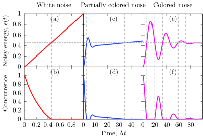
Figure 1: (Color online) The figure shows a comparison between the noisy energy of one of the oscillators [Eq. (9)] and concurrence (entanglement) for noise with different memory. The initial state is $(\ket{01}+\ket{10})/\sqrt{2}$. When the energy exceeds (falls below) the threshold $0.455\,\omega$, there is sudden death (rebirth) of entanglement. (a,b) use $\Lambda\tau=0$; (c,d) $\omega\tau=3.5$ and $\omega/\Lambda=0.875$; (e,f) $\omega\tau=7.5$ and $\omega/\Lambda=0.25$.

In this work, we present an exactly solvable model involving two independent harmonic oscillators each interacting with its own classical non-Markovian stochastic reservoir. No back-reaction to the reservoirs is considered. This system has the property that it can be solved analytically allowing us to study non-Markovian effects on the dynamics of entanglement including the prolonging of entanglement and its rebirth. Particularly, we study the dynamics of entanglement for the lowest two states of the oscillators which form a qubit-like system. Curiously, there is a one-to-one correspondence between the amount of energy added to each oscillator from the noise source and their entanglement: As the energy increases (decreases) across a threshold, we see sudden death (rebirth) of entanglement (see Fig. 1). Furthermore, this initial-state dependent threshold is independent of the form of the noise correlations in time because all memory effects enter via the energy of a single oscillator which in turn encodes the memory effects.

Entanglement between harmonic oscillators can be quantified in several ways Prauzner-Bechcicki (2004) and can be produced on demand with trapped ion systems Turchette et al. (1998). Here we focus on the lowest two states of each oscillator which form a two qubit-like Hilbert subspace. For a two qubit-like system, entanglement is unambiguously quantified in terms of the concurrence $C(\hat{\varrho}_{2}(t))$, where $\hat{\varrho}_{2}$ is the density matrix of two qubit system, we have

$$C(t)=\max\{0,\sqrt{\lambda_{1}}-\sqrt{\lambda_{2}}-\sqrt{\lambda_{3}}-\sqrt{\lambda_{4}}\},$$ (1)

where $\lambda_{i}$ are the eigenvalues (in decreasing order) of the matrix $\hat{\varrho}_{2}(t)\tilde{\varrho}_{2}(t)$ where $\tilde{\varrho}_{2}=(\sigma_{y}\otimes\sigma_{y})\hat{\varrho}_{2}^{*}(\sigma_{y}\otimes\sigma_{y})$. Physically, it can be shown Wootters (1998) that states are maximally entangled if $C(t)=1$ and completely disentangled for $C(t)=0$. When $C(t)=0$ there exists a realization of $\hat{\varrho}_{2}(t)$ such that $\hat{\varrho}_{2}(t)=\sum_{k}p_{k}\ket{\psi_{k}}\bra{\psi_{k}}$ where every $\ket{\psi_{k}}$ is separable; i.e., the system is a classical mixture of separable states. The concurrence can vanish or appear suddenly at a finite time, counter to what one may naively expect from the exponential decay of coherences (with characteristic time $T_{2}$) which are local quantum phenomena.

In the course of our analysis we first develop the tools to compute the noise-average density matrix for a single oscillator in the presence of non-Markovian drive. In addition, we calculate the probability distribution functions (PDFs) of position, momentum, and energy observables – completely characterizing the non-Markovian statistics of such a system.

In Section II we introduce the system and notation, and we calculate some basic quantities including correlation functions and energy. In particular, the energy added to the system by the bath $\epsilon(t)$ (see Fig. 2) controls all memory effects that show up in all later parts of the analysis (including concurrence, as illustrated in Fig. 1). In Section II.1 we analytically compute the noise-averaged density matrix (Eq. (32)) for a single oscillator in the presence of non-Markovian noise using a combination of functional integral and Lie algebraic techniques. In Section II.2, we calculate the PDFs of position, momentum, and energy. We find Gaussian PDFs for position and momentum and an exponential PDF for energy. These PDFs are intimately controlled by $\epsilon(t)$; they can even contract back towards a delta function for finite intervals of time before spreading in a diffusive behavior. In Section III we study the evolution of concurrence for two oscillators initially maximally entangled (see Eq. (58)) in the subspace of their two lowest states. The oscillators are independent and subject to independent sources of non-Markovian noise. We apply the machinery developed in Section II and find an analytical expression for the effective two-qubit-like density matrix (Eq. (59)) used to calculate the concurrence. We conclude in Section IV with a summary of the main results derived in this work shown explicitly in Table 1.

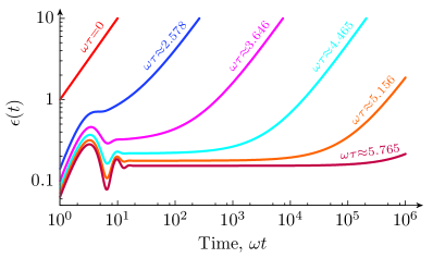
Figure 2: (Color online) The plot is the function $\epsilon(t)$ which appears in the energy of the oscillator [Eq. (9)], the variances in $\hat{x}$ and $\hat{p}$ [Eq. (10)], the probability distribution functions of position, momentum [Eq. (42)], and energy [Eq. (55)], and the density matrix [Eq. (32)]. This plot uses $\omega=\Lambda$.

II Single oscillator statistics

In order to study the statistics of a single oscillator, we first define our system and calculate some basic quantities before moving onto the bulk of the calculations in Section II.1 and II.2. In particular, the energy added to the system by noise will be important in much of our analysis. The results of this section are extended to the problem of entanglement of two oscillators in Section III.

Our system is characterized by the Hamiltonian of a single driven harmonic oscillator ($\hbar=1$)

$$\hat{H}=\omega(a^{\dagger}a+\tfrac{1}{2})+\tfrac{1}{\sqrt{2}}[\xi(t)a^{\dagger}+\mathrm{h.c.}],$$ (2)

where $a^{\dagger}(a)$ are the standard creation (annihilation) operators with $[a,a^{\dagger}]=1$ and $\xi(t)=\xi_{1}(t)+i\xi_{2}(t)$ defines our external stochastic noise $\xi_{1,2}$ which are turned on after $t=0$. The stochastic forcing terms are completely characterized by their mean $\langle\xi_{i}(t)\rangle_{\xi}=0$ and two-time correlation functions

$$\langle\xi_{i}(t)\xi_{j}(t^{\prime})\rangle_{\xi} =K_{ij}(t,t^{\prime})=\delta_{ij}k(t-t^{\prime})$$

$$=\delta_{ij}\tfrac{\Lambda}{\tau\sqrt{2\pi}}\,\mathrm{e}^{-(t-t^{\prime})^{2}/2\tau^{2}},$$ (3)

Our analytical results do not depend on the explicit functional form of the correlation function $k(t-t^{\prime})$, but plots and physical explanations will use the Gaussian time correlations with amplitude $\Lambda$ and time-correlations $\tau$. For $\tau=0$, the noise has no memory and this leads to well known Markovian behavior Breuer and Petruccione (2002). We are mostly concerned with the regime where $\tau\neq 0$. The average over noise is defined as the functional integral,

$$\braket{(\cdots)}_{\xi} =\frac{\int\mathcal{D}^{2}\xi\,(\cdots)\mathrm{e}^{-\frac{1}{2}\int_{0}^{t}dt^{\prime}\int_{0}^{t}dt^{\prime\prime}\xi_{i}(t^{\prime})K^{-1}_{ij}(t^{\prime},t^{\prime\prime})\xi_{j}(t^{\prime\prime})}}{\int\mathcal{D}^{2}\xi\,\mathrm{e}^{-\frac{1}{2}\int_{0}^{t}dt^{\prime}\int_{0}^{t}dt^{\prime\prime}\xi_{i}(t^{\prime})K^{-1}_{ij}(t^{\prime},t^{\prime\prime})\xi_{j}(t^{\prime\prime})}},$$ (4)

(summing over repeated indices) where $K^{-1}$ represents the inverse integral kernel of $K$.

We define the standard occupation number $\hat{n}=a^{\dagger}a$, position $\hat{x}=(a+a^{\dagger})/\sqrt{2}$ and momentum $\hat{p}=(a-a^{\dagger})/(\sqrt{2}i)$ operators. The matrix $R$ is a $2\times 2$ rotation matrix

$$R(t)=\begin{pmatrix}\cos\omega t&\sin\omega t\\ -\sin\omega t&\cos\omega t\end{pmatrix}.$$ (5)

We first study non-Markovian effects in the correlation functions of position and momentum. The equation of motion for the position and momentum operators in the Heisenberg picture are $\partial_{t}\hat{x}(t)=\omega\hat{p}(t)+\xi_{2}(t)$ and $\partial_{t}\hat{p}(t)=-\omega\hat{x}(t)-\xi_{1}(t)$. Define $\hat{\mathbf{V}}(t)=(-\hat{p}(t),\hat{x}(t))^{T}$ as a two component vector then solutions can be written as

$$\hat{\mathbf{V}}(t)=R(t)\hat{\mathbf{V}}(0)+\int_{\mathrlap{0}}^{\mathrlap{t}}ds\,R(t-s)\bm{\xi}(s)$$ (6)

where $\bm{\xi}(t)=(\xi_{1}(t),\xi_{2}(t))^{T}$ is the external drive. With these definitions and assuming that the oscillator is initially in a number state $\ket{n}$ the noise-averaged correlation functions are

$$\langle\langle\hat{\mathbf{V}}(t)\hat{\mathbf{V}}^{T}(t^{\prime})\rangle\rangle_{\xi}=R(t)\langle\hat{\mathbf{V}}(0)\hat{\mathbf{V}}^{T}(0)\rangle R(-t^{\prime})\\ +\int_{\mathrlap{0}}^{\mathrlap{t}}ds\int_{\mathrlap{0}}^{\mathrlap{t^{\prime}}}ds^{\prime}\,R(t-s)K(s,s^{\prime})R(s^{\prime}-t^{\prime}).$$ (7)

where $\left\langle\cdots\right\rangle$ is the quantum mechanical expectation value and $\langle\cdots\rangle_{\xi}$ is the average over noise. In particular, from Eq. (7) the average of the energy is $\langle\langle\hat{E}(t)\rangle\rangle_{\xi}=\omega\langle\langle\hat{x}^{2}(t)+\hat{p}^{2}(t)\rangle\rangle_{\xi}/2=\omega\langle\langle\operatorname{{\mathrm{t}r}}[\hat{\mathbf{V}}(t)\hat{\mathbf{V}}^{T}(t)]\rangle\rangle_{\xi}/2$. Defining the energy added to the system due to noise as $\omega\epsilon(t)=\langle\langle\hat{E}(t)\rangle\rangle_{\xi}-\langle\langle\hat{E}(0)\rangle\rangle_{\xi}=\langle\langle\hat{E}(t)\rangle\rangle_{\xi}-\omega(n+1/2)$ we find

$$\epsilon(t) =\frac{1}{2}\int_{\mathrlap{0}}^{\mathrlap{t}}ds\int_{\mathrlap{0}}^{\mathrlap{t}}ds^{\prime}\,\operatorname{{\mathrm{t}r}}\{R(t-s)K(s,s^{\prime})R(s^{\prime}-t)\}$$ (8)

$$=\int_{\mathrlap{0}}^{\mathrlap{t}}ds\int_{\mathrlap{0}}^{\mathrlap{t}}ds^{\prime}\,\cos\omega(s-s^{\prime})k(s-s^{\prime})$$ (9)

Defining $\Sigma^{2}_{p}(t)=\langle\langle\hat{p}(t)\rangle^{2}\rangle_{\xi}-\langle\langle\hat{p}(t)\rangle\rangle_{\xi}^{2}$ and similarly for the position operator we find

$$\Sigma^{2}_{p}(t)=\Sigma^{2}_{x}(t)=\epsilon(t).$$ (10)

We see that the variances of position and momentum with respect to noise are controlled by the function $\epsilon(t)$ which is the energy added to the system after stochastic forcing is turned on. In Section II.2 we generalize these results and obtain all moments of the noise-averaged position, momentum, and energy. The complete distribution for position and momentum is Gaussian and determined by its mean and variance. On the other hand, the distribution for energy is exponential and thus characterized by its mean and initial value. The noise-averaged energy of the oscillator $\epsilon(t)$ appears frequently in our statistical analysis.

If we consider Gaussian time-correlations, $\epsilon(t)$ has a closed form in terms of error functions. However, to see its qualitative properties, consider its derivatives. For the case of a Gaussian noise (Eq. (3)),

$$\frac{d\epsilon(t)}{dt}\xrightarrow{t\rightarrow\infty}\Lambda\mathrm{e}^{-\omega^{2}\tau^{2}/2}.$$ (11)

This means that at long times the behavior is linear with slope $\Lambda e^{-\omega^{2}\tau^{2}/2}$. The slope is exponentially small in $\tau$ with scale given by $1/\omega$. Thus, memory in the bath exponentially suppresses the rate of energy transfer from bath to system at long times. From the second derivative

$$\frac{d^{2}\epsilon(t)}{dt^{2}}=\frac{2\Lambda}{\tau\sqrt{2\pi}}e^{-t^{2}/2\tau^{2}}\cos\omega t,$$ (12)

we see that there are inflection points equally spaced in time which means that at short times there are oscillations with fixed frequency $\omega$ and their initial amplitude is of the order of $\Lambda$. It also shows that the amplitude of such oscillations decay as time increases with time scale $\tau$. The longer the memory of the noise the longer the oscillations are prolonged. The short time oscillations and long time linear growth are shown in Fig. 2. This behavior is generic to any noise correlation function that decays fast enough. To understand this, after a change of variables Eq. (9) becomes

$$\epsilon(t)=t\int_{-\mathrlap{t}}^{\mathrlap{t}}du\,k(u)\cos\omega u-\int_{-\mathrlap{t}}^{\mathrlap{t}}du\,|u|k(u)\cos\omega u.$$ (13)

At long times $\epsilon(t)$ is linear and the first term in Eq. (13) gives the slope of $\epsilon(t)$ as $t\rightarrow\infty$ Maniscalco et al. (2004).

With these basic quantities defined and calculated, we can now find the full quantum and statistical dynamics of the system characterized by the density matrix and probability distribution functions.

II.1 The noise-averaged density matrix

The density matrix captures both the quantum and statistical nature of a system, and in order to calculate it, we employ functional integral and Lie algebraic methods illustrated in this section.

The evolution operator for a single harmonic oscillator obeys the equation $i\partial_{t}\hat{U}=\hat{H}(t)\hat{U}(t)$ with $\hat{U}(0)=\hat{1}$, and is given by Galitski (2011)

$$\hat{U}(t)=\mathrm{e}^{-i\omega t(\hat{n}+1/2)}\mathrm{e}^{-i(\Phi_{1}(t)\hat{x}+\Phi_{2}(t)\hat{p})}\mathrm{e}^{i\gamma(t)}.$$ (14)

where $\Phi_{i}(t)=\int_{0}^{t}ds\,\xi_{j}(s)R_{ji}(s)$. We define the noise-averaged density matrix by

$$\hat{\rho}(t)=\langle\hat{U}(t)\hat{\rho}(0)\hat{U}^{\dagger}(t)\rangle_{\xi}\equiv\mathrm{e}^{\mathcal{L}(t)}\hat{\rho}(0),$$ (15)

where $\hat{\rho}(0)$ is the initial density matrix. It is convenient to express the evolution of the density matrix via a quantum ‘Liouvillian’ operator $\mathcal{L}(t)$. Using $\mathrm{e}^{\hat{A}}\hat{B}\mathrm{e}^{-\hat{A}}=\mathrm{e}^{\operatorname{{\mathrm{a}d}}_{\hat{A}}}\hat{B}$ where $\operatorname{{\mathrm{a}d}}_{\hat{A}}\hat{B}=[\hat{A},\hat{B}]$ is the (linear) adjoint operator, we obtain

$$\mathrm{e}^{\mathcal{L}(t)}=\mathrm{e}^{-i\omega t\operatorname{{\mathrm{a}d}}_{\hat{n}}}\braket{\mathrm{e}^{-i(\Phi_{1}(t)\operatorname{{\mathrm{a}d}}_{\hat{x}}+\Phi_{2}(t)\operatorname{{\mathrm{a}d}}_{\hat{p}})}}_{\xi}.$$ (16)

Note that $[\operatorname{{\mathrm{a}d}}_{\hat{x}},\operatorname{{\mathrm{a}d}}_{\hat{p}}]=0$ and $[\operatorname{{\mathrm{a}d}}_{\hat{x}},1]=0=[\operatorname{{\mathrm{a}d}}_{\hat{p}},1]$ allow us to treat $\operatorname{{\mathrm{a}d}}_{\hat{x}}$ and $\operatorname{{\mathrm{a}d}}_{\hat{p}}$ as $c$-numbers when integrating over $\xi_{1,2}$. Suppressing normalization, indices, and integration for clarity, we obtain

$$\hat{\rho}(t) =\mathrm{e}^{-i\omega t\operatorname{{\mathrm{a}d}}_{\hat{n}}}\left[\int\mathcal{D}^{2}\xi\;\mathrm{e}^{-i\int\bm{\xi}^{T}R\operatorname{{\mathrm{a}d}}_{\hat{\mathbf{X}}}}\mathrm{e}^{-\frac{1}{2}\iint\bm{\xi}^{T}K^{-1}\bm{\xi}}\right]\hat{\rho}(0)$$

$$=\mathrm{e}^{-i\omega t\operatorname{{\mathrm{a}d}}_{\hat{n}}}\mathrm{e}^{-\frac{1}{2}\operatorname{{\mathrm{a}d}}_{\hat{\mathbf{X}}}^{T}\left[\iint R^{T}KR\right]\operatorname{{\mathrm{a}d}}_{\hat{\mathbf{X}}}}\hat{\rho}(0),$$ (17)

where $\operatorname{{\mathrm{a}d}}_{\hat{\mathbf{X}}}=(\operatorname{{\mathrm{a}d}}_{\hat{x}},\operatorname{{\mathrm{a}d}}_{\hat{p}})^{T}$. In Eq. (17), we note that the set of operators $\{\frac{1}{2}\operatorname{{\mathrm{a}d}}_{\hat{n}},\operatorname{{\mathrm{a}d}}_{\hat{x}}^{2}+\operatorname{{\mathrm{a}d}}_{\hat{p}}^{2},\operatorname{{\mathrm{a}d}}_{\hat{x}}^{2}-\operatorname{{\mathrm{a}d}}_{\hat{p}}^{2},2\operatorname{{\mathrm{a}d}}_{\hat{x}}\operatorname{{\mathrm{a}d}}_{\hat{p}}\}$ surprisingly form a Lie algebra (see Appendix A). This can be used to derive a full equation of motion for the density matrix.

Considering our particular form of noise, explicit calculation gives

$$\operatorname{{\mathrm{a}d}}_{\hat{\mathbf{X}}}^{T}\left[\iint R^{T}KR\right]\operatorname{{\mathrm{a}d}}_{\hat{\mathbf{X}}} =\epsilon(t)(\operatorname{{\mathrm{a}d}}_{\hat{x}}^{2}+\operatorname{{\mathrm{a}d}}_{\hat{p}}^{2}),$$ (18)

where $\epsilon(t)$ is given by Eq. (9).

To make further progress we need some facts about operators that act in this Hilbert space. We know that any operator $\hat{\mathcal{O}}$ can be expanded (Appendix A) as

$$\hat{\mathcal{O}}=\int\frac{dy\,dq}{2\pi}\operatorname{{\mathrm{t}r}}[\hat{\mathcal{O}}\mathrm{e}^{iy\hat{p}-iq\hat{x}}]\mathrm{e}^{iq\hat{x}-iy\hat{p}},$$ (19)

and the operators $\mathrm{e}^{iq\hat{x}-iy\hat{p}}$ are eigenoperators of the operators $\operatorname{{\mathrm{a}d}}_{\hat{x}}$ and $\operatorname{{\mathrm{a}d}}_{\hat{p}}$:

$$\operatorname{{\mathrm{a}d}}_{\hat{x}}\mathrm{e}^{iq\hat{x}-iy\hat{p}} =y\,\mathrm{e}^{iq\hat{x}-iy\hat{p}},$$ (20)

$$\operatorname{{\mathrm{a}d}}_{\hat{p}}\mathrm{e}^{iq\hat{x}-iy\hat{p}} =q\,\mathrm{e}^{iq\hat{x}-iy\hat{p}}.$$ (21)

Further, we can calculate the matrix element (Appendix B)

$$\braket{n}{\mathrm{e}^{iy\hat{p}-iq\hat{x}}}{m} =\sqrt{\frac{n!}{m!}}(z^{*})^{m-n}L_{n}^{(m-n)}(|z|^{2})\mathrm{e}^{-|z|^{2}/2},$$ (22)

where $z\equiv(y+iq)/\sqrt{2}$ and $L_{n}^{(m)}$ is an associated Laguerre polynomial. Also, $\operatorname{{\mathrm{a}d}}_{\hat{x}}^{2}+\operatorname{{\mathrm{a}d}}_{\hat{p}}^{2}$ commutes with $\operatorname{{\mathrm{a}d}}_{\hat{n}}$ (Appendix A). The density matrix can be expanded as $\hat{\rho}(0)=\sum_{mn}\rho_{mn}\ket{m}\bra{n}$ where $\rho_{mn}=\bra{m}\hat{\rho}(0)\ket{n}$ and therefore we only need to calculate the evolution of the basis elements $\ket{m}\bra{n}$.

Combining the above facts, we obtain from Eq. (19) that

$$\mathrm{e}^{\mathcal{L}(t)}\ket{m}\bra{n}=\mathrm{e}^{-i\omega t(m-n)}\int\frac{dy\,dq}{2\pi}\braket{n}{\mathrm{e}^{iy\hat{p}-iq\hat{x}}}{m}\\ \times\mathrm{e}^{iq\hat{x}-iy\hat{p}}\mathrm{e}^{-\frac{1}{2}\epsilon(t)(q^{2}+y^{2})}.$$ (23)

To evaluate this, we calculate the matrix element $\braket{k}{\{\mathrm{e}^{\mathcal{L}(t)}\ket{m}\bra{n}\}}{l}$; using Eq. (22) and shifting to polar coordinates $z=\sqrt{x}\mathrm{e}^{i\theta}$ such that $d^{2}z=\frac{1}{2}dx\,d\theta$ we obtain

$$\braket{k}{\{\mathrm{e}^{\mathcal{L}(t)}\ket{m}\bra{n}\}}{l}=\sqrt{\frac{n!l!}{m!k!}}\mathrm{e}^{-i\omega t(m-n)}\\ \times\int_{\mathrlap{0}}^{\mathrlap{\infty}}dx\int_{\mathrlap{0}}^{2\pi}\frac{d\theta}{2\pi}x^{(k-l+m-n)/2}\mathrm{e}^{i\theta(k-l-m+n)}\\ \times L_{n}^{(m-n)}(x)L_{l}^{(k-l)}(x)\mathrm{e}^{-(1+\epsilon(t))x},$$ (24)

for which we can integrate $\theta$ to obtain

$$\braket{k}{\{\mathrm{e}^{\mathcal{L}(t)}\ket{m}\bra{n}\}}{l}=\sqrt{\frac{n!l!}{m!k!}}\delta_{k-l,m-n}\mathrm{e}^{-i\omega t(m-n)}\\ \times\int_{\mathrlap{0}}^{\mathrlap{\infty}}dx\,x^{m-n}L_{n}^{(m-n)}(x)L_{l}^{(m-n)}(x)\mathrm{e}^{-(1+\epsilon(t))x}.$$ (25)

On the other hand, using the identity

$$\frac{(-x)^{m}}{m!}L_{n}^{(m-n)}(x)=\frac{(-x)^{n}}{n!}L_{m}^{(n-m)}(x),$$ (26)

we can rewrite Eq. (24) as

$$\braket{k}{\{\mathrm{e}^{\mathcal{L}(t)}\ket{m}\bra{n}\}}{l}=\sqrt{\frac{m!k!}{n!l!}}\delta_{k-l,m-n}\mathrm{e}^{-i\omega t(m-n)}\\ \times\int_{\mathrlap{0}}^{\mathrlap{\infty}}dx\,x^{n-m}L_{m}^{(n-m)}(x)L_{k}^{(n-m)}(x)\mathrm{e}^{-(1+\epsilon(t))x}.$$ (27)

The right hand side (RHS) of Eq. (27) is the same expression as the RHS of Eq. (25) with $n\leftrightarrow m$ and $k\leftrightarrow l$ (except for the multiplicative $\mathrm{e}^{-i\omega t(m-n)}$ term). Thus, we can use Eq. (25) and assume $m\geq n$ without loss of generality. At the end of our calculation, we simply switch indices to obtain $m\leq n$.

A change of variables $y=(1+\epsilon(t))x$ in Eq. (25) yields

$$\braket{k}{\{\mathrm{e}^{\mathcal{L}(t)}\ket{m}\bra{n}\}}{l}=\sqrt{\frac{n!l!}{k!m!}}\frac{\delta_{k-l,m-n}\mathrm{e}^{-i\omega t(m-n)}}{(1+\epsilon(t))^{m-n+1}}\\ \times\int_{\mathrlap{0}}^{\mathrlap{\infty}}dy\,y^{m-n}L_{n}^{(m-n)}\left(\tfrac{y}{1+\epsilon(t)}\right)L_{l}^{(m-n)}\left(\tfrac{y}{1+\epsilon(t)}\right)\mathrm{e}^{-y}.$$ (28)

Together with the property of Laguerre polynomials

$$L_{n}^{(m-n)}\left(\tfrac{y}{1+\epsilon(t)}\right)=\sum_{i=0}^{n}\frac{\epsilon(t)^{n-i}}{(1+\epsilon(t))^{n}}\binom{m}{n-i}L_{i}^{(m-n)}(y),$$ (29)

we obtain

$$\int_{\mathrlap{0}}^{\mathrlap{\infty}}dy\,y^{m-n}L_{n}^{(m-n)}\left(\tfrac{y}{1+\epsilon(t)}\right)L_{l}^{(m-n)}\left(\tfrac{y}{1+\epsilon(t)}\right)\mathrm{e}^{-y}\\ =\frac{\epsilon(t)^{n+l}}{(1+\epsilon(t))^{n+l}}\binom{m}{n}\binom{l+m-n}{l}(m-n)!\\ \times\tensor{[}_{2}]{F}{{}_{1}}[-l,-n;1+m-n;\epsilon(t)^{-2}],$$ (30)

where $\tensor{[}_{2}]{F}{{}_{1}}$ is the hypergeometric function. Thus, we can return to Eq. (28) to obtain $\braket{k}{\{\mathrm{e}^{\mathcal{L}(t)}\ket{m}\bra{n}\}}{l}$ and hence $\mathrm{e}^{\mathcal{L}(t)}\ket{m}\bra{n}$ expanded in the number basis. Then, given an arbitrary initial density matrix

$$\hat{\rho}(0)=\sum_{mn}\rho_{mn}\ket{m}\bra{n},$$ (31)

we have the time-evolved, noise-averaged density matrix

$$\hat{\rho}(t)=\sum_{\mathclap{n,m=0}}^{\infty}\rho_{m+n,n}\mathrm{e}^{-i\omega tm}\sum_{l=0}^{\infty}\sqrt{\frac{(m+n)!(l+m)!}{n!l!}}\frac{\epsilon(t)^{n+l}\tensor{[}_{2}]{F}{{}_{1}}[-l,-n;1+m;\epsilon(t)^{-2}]}{m!(1+\epsilon(t))^{m+n+l+1}}\ket{l+m}\bra{l}\\ +\sum_{\mathclap{\begin{subarray}{c}n=1\\ m=0\end{subarray}}}^{\infty}\rho_{m,n+m}\mathrm{e}^{i\omega tn}\sum_{l=0}^{\infty}\sqrt{\frac{(n+m)!(l+n)!}{m!l!}}\frac{\epsilon(t)^{m+l}\tensor{[}_{2}]{F}{{}_{1}}[-l,-m;1+n;\epsilon(t)^{-2}]}{n!(1+\epsilon(t))^{n+m+l+1}}\ket{l}\bra{l+n}.$$ (32)

Note that Eq. (32) only depends on time through the energy added by noise $\epsilon(t)$ and a phase factor. To get a feeling for what Eq. (32) means consider an oscillator in the initial state $\ket{3}$, so $\hat{\rho}(0)=\ket{3}\bra{3}$ and

$$\hat{\rho}(t) =\sum_{l}p_{l}[\epsilon(t)]\ket{l}\bra{l}$$ (33)

with $p_{l}[\epsilon(t)]$ being the probability of being in state $\ket{l}$ at time $t$,

$$p_{l}[x] =\tfrac{x^{l-3}[6x^{6}+18lx^{4}+9l(l-1)x^{2}+l(l-1)(l-2)]}{6(1+x)^{l+4}}.$$ (34)

The results are plotted in Fig. 3. Since the horizontal axis is $\epsilon(t)$, the non-Markovian oscillations at short times can cause oscillations in the evolution of $p_{l}[\epsilon(t)]$. This will be important when we consider entanglement between two oscillators in Section III.

The noise-average of any observable can be obtained by $\langle\langle\hat{X}\rangle\rangle_{\xi}=\textrm{tr}\{\hat{\rho}(t)\hat{X}\}$ with $\hat{\rho}(t)$ given by Eq. (32). The analytical computation of this quantity is one of our main results. An alternative description which makes explicit the statistics of a particular observable is via its probability distribution function which we calculate in the next section.

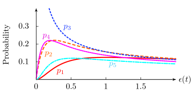
Figure 3: (Color online) The above is the [classical] probability $p_{l}$ of the oscillator being in state $\ket{l}$ if its initial state was $\ket{3}$ vs. the oscillator energy $\epsilon(t)$ [Eq. (33)].

II.2 Probability distribution functions

The random drive acting on the oscillator introduces uncertainty in the quantum mechanical observables in addition to the quantum mechanical spread of the system observables. The effect of the random drive on an observable can be completely characterized by its probability distribution function (PDF). For an operator $\hat{A}$ with quantum mechanical average $\langle\hat{A}\rangle$ its PDF, is

$$P_{\hat{A}}[A;t]=\langle\delta[A-\braket{\hat{A}(t)}]\rangle_{\xi}.$$ (35)

With this definition, we analytically compute the PDF of position, momentum, and energy with Gaussian noise.

II.2.1 Position and momentum probability distribution functions

The quantum mechanical average of position or momentum has the form

$$\braket{\hat{A}(t)}=X(t)+\int_{\mathrlap{0}}^{\mathrlap{t}}dt^{\prime}\,g_{i}(t,t^{\prime})\xi_{i}(t^{\prime}).$$ (36)

For the moment we leave unspecified the functions $X(t)$ and $g_{i}(t,t^{\prime})$. The first term is the quantum mechanical average of the operator in the absence of stochastic drive, e.g., from the first term in Eq. (6) while the second term gives the contribution due to the random drive. This approach can be applied to any operator that conforms to this form. The Dirac delta can be represented as an integral $\delta(x)=\int\mathrm{e}^{iux}(du/2\pi)$ to obtain

$$P_{\hat{A}}[A;t]=\int\frac{du}{2\pi}\int\mathcal{D}^{2}\xi(t)\,\mathrm{e}^{-\frac{1}{2}\iint\bm{\xi}^{T}K^{-1}\bm{\xi}-iu\int\mathbf{g}^{T}\bm{\xi}}\\ \times\mathrm{e}^{iu(A-X(t))},$$ (37)

where $\mathbf{g}=(g_{1},g_{2})^{T}$ and $\bm{\xi}=(\xi_{1},\xi_{2})^{T}$. The above is a quadratic path integral and can thus be solved exactly by standard techniques. Throughout, we use the fact that $K_{ij}(t,t^{\prime})=K_{ji}(t^{\prime},t)$. Explicit calculation gives

$$P_{\hat{A}}[A;t] =\int\frac{du}{2\pi}\mathrm{e}^{-\frac{u^{2}}{2}\iint\mathbf{g}^{T}K\mathbf{g}+iu(A-X(t))}$$

$$=\frac{1}{\sqrt{2\pi}\Sigma_{A}(t)}\exp\left\{-\frac{[A-X(t)]^{2}}{2\Sigma_{A}^{2}(t)}\right\},$$ (38)

where the variance of the PDF is

$$\Sigma_{A}^{2}(t)=\int_{\mathrlap{0}}^{\mathrlap{t}}dt_{1}\int_{\mathrlap{0}}^{\mathrlap{t}}dt_{2}\,g_{i}(t,t_{1})K_{ij}(t_{1},t_{2})g_{j}(t,t_{2}).$$ (39)

The form of $g_{i}$ depends on $\hat{A}$ (Eq. (36)); for the position operator $g_{1}(t,s)=-\sin\omega(t-s)$, $g_{2}(t,s)=\cos\omega(t-s)$ and for the momentum operator $g_{1}(t,s)=-\cos\omega(t-s)$, $g_{2}(t,s)=-\sin\omega(t-s)$ [these are taken directly from the $R(t-s)\bm{\xi}$ term in Eq. (6)]. From Eq. (38) and given that the oscillator is in an initial coherent state $\ket{z_{0}}$ where $z_{0}=(x_{0}+ip_{0})/\sqrt{2}$, we obtain

$$P_{\hat{x}}[X;t] =\frac{1}{\sqrt{2\pi}\Sigma_{x}(t)}\exp\left\{-\frac{[X-X_{\mathrm{cl}}(t)]^{2}}{2\Sigma_{x}(t)^{2}}\right\},$$ (40)

$$P_{\hat{p}}[P;t] =\frac{1}{\sqrt{2\pi}\Sigma_{p}(t)}\exp\left\{-\frac{[P-P_{\mathrm{cl}}(t)]^{2}}{2\Sigma_{p}(t)^{2}}\right\},$$ (41)

where the variances are the same as in Eq. (10), i.e.,

$$\Sigma^{2}_{x,p}(t)=\epsilon(t)$$ (42)

where $X,P$ are random variables of position and momentum. We see that they are normally distributed about the solutions of the classical equations of motion; $X_{\mathrm{cl}}(t)=x_{0}\cos\omega t+p_{0}\sin\omega t$ and $P_{\mathrm{cl}}(t)=-x_{0}\sin\omega t+p_{0}\cos\omega t$ (see Fig. 4(a)).

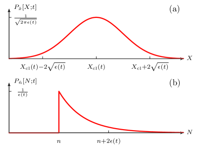
Figure 4: (a) The probability distribution function for the position operator [Eq. (40)] is shown. The probability distribution function for momentum is the same except with a different center [$P_{\mathrm{cl}}(t)$ instead of $X_{\mathrm{cl}}(t)$]. (b) The probability distribution function of the energy or, equivalently, number operator [Eq. (55)] is shown.

Hence we see that $\langle\langle\hat{x}(t)\rangle\rangle_{\xi}$ and $\langle\langle\hat{p}(t)\rangle\rangle_{\xi}$ will satisfy the standard classical equations of motion for the harmonic oscillator.

It is important to note that memory effects are all included analytically in Eq. (42). The spread in the uncertainty is in fact in one-to-one correspondence with the behavior of the energy of the oscillator. This means that for white noise ($k(t)=\Lambda\delta(t)$) there is a Brownian (in time) increase in the variance of the PDF of position and momentum, $\Sigma_{x,p}(t)=\sqrt{\Lambda t}$, which is expected for a Markovian-type of noise. If the memory of the noise is nonzero, the behavior is non-monotonic and the uncertainty in the position and momentum can decrease at times making the system more deterministic than random. This is counter to what one might naively expect from a noise source and shows the importance of memory. In the extreme case of non-decaying noise correlations ($k(t)=\Lambda$), we have $\Sigma^{2}_{x,p}(t)=2\Lambda(1-\cos\omega t)/\omega^{2}$ which means that the PDFs $P_{\hat{x}}[X,2\pi k/\omega]$ and $P_{\hat{p}}[P,2\pi k/\omega]$ (with $k$ an integer) collapse into delta functions. At these discrete times, the expectation value of these observables will yield the classical value of position and momentum and purely quantum mechanical behavior is restored. Thus, even for finite, but long time-correlations, the position of $x$ can stay localized for quite a long time (as seen by the exponential suppression $e^{-\omega^{2}\tau^{2}/2}$ of the growth of the variance). Intuitively, the system remembers its initial pure state and tries to restore it. When the memory is finite, this restoration is not complete but still can give non-monotonic behavior. Nonetheless, at large times we recover Brownian-type behavior (see Fig. 2).

II.2.2 Energy probability distribution function

Formally consider the quantity

$$\braket{\hat{B}(t)}=X(t)+\frac{1}{2}\int_{\mathrlap{0}}^{\mathrlap{t}}dt_{1}\int_{\mathrlap{0}}^{\mathrlap{t}}dt_{2}\,\xi_{i}(t_{1})F_{ij}(t_{1},t_{2})\xi_{j}(t_{2}),$$ (43)

where the function $X(t)$ and matrix $F(t)$ are unspecified for the moment. This is the case for the quantum expectation value of the energy. In this case explicit calculation gives,

$$P_{\hat{B}}[B;t]=\int\frac{du}{2\pi}\frac{1}{\sqrt{\det{K}}}\int\mathcal{D}^{2}\xi(t)\,\\ \times\mathrm{e}^{-\frac{1}{2}\iint\bm{\xi}^{T}\left[K^{-1}+iuF\right]\bm{\xi}+iu(B-X(t))}$$ (44)

Evaluating this quadratic path integral yields

$$P_{\hat{B}}[B;t]=\int\frac{du}{2\pi}\frac{\mathrm{e}^{iu(B-X(t))}}{\sqrt{\det[1+iuKF]}}.$$ (45)

The determinants can be viewed in the following way: To find “$\det D(t_{1},t_{2})$” take the function $D(t_{1},t_{2})$ and time slice it $N-1$ times from $0$ to $t$, so one has an $N\times N$ matrix. Find the determinant of this matrix, then let $N\rightarrow\infty$. The quantities $1+iuKF$ and $K$ are also $2\times 2$ matrices, and in that case one just takes the determinant of the matrix created by the direct product of those two spaces ($2N\times 2N$ matrices). Again, we use the fact that $K_{ij}(t_{1},t_{2})=K_{ji}(t_{2},t_{1})$ and further, we assume $F_{ij}(t_{1},t_{2})=F_{ji}(t_{2},t_{1})$.

For the specific case of the energy PDF we compute this determinant using methods developed in Section II.1. Assuming the system is initially in a number state $\ket{n}$, the average occupation number in the presence of the external drive is

$$\braket{\hat{n}(t)}=n+\frac{1}{2}\int_{\mathrlap{0}}^{\mathrlap{t}}dt_{1}\int_{\mathrlap{0}}^{\mathrlap{t}}dt_{2}\,\xi_{i}(t_{1})R_{ij}(t_{1}-t_{2})\xi_{j}(t_{2}),$$ (46)

and using Eq. (45)

$$P_{\hat{n}}[N;t]=\int\frac{du}{2\pi}\sqrt{\frac{1}{\det[1+iuKR]}}\,\mathrm{e}^{iu(N-n)}.$$ (47)

By going a step back, the determinant can be written as

$$\sqrt{\frac{1}{\det[1+iuKR]}}=\braket{\mathrm{e}^{-\frac{1}{2}iu\xi^{T}R\xi}}_{\xi}.$$ (48)

Now, let us consider the following quantity

$$\braket{\braket{0}{\{{\mathrm{e}^{-iz(\Phi_{1}(t)\operatorname{{\mathrm{a}d}}_{\hat{x}}+\Phi_{2}(t)\operatorname{{\mathrm{a}d}}_{\hat{p}})}}\ket{0}\bra{0}\}}{0}}{}{\xi}\\ =\braket{0}{\{\braket{\mathrm{e}^{-iz(\Phi_{1}(t)\operatorname{{\mathrm{a}d}}_{\hat{x}}+\Phi_{2}(t)\operatorname{{\mathrm{a}d}}_{\hat{p}})}}_{\xi}\ket{0}\bra{0}\}}{0},$$ (49)

The left hand side of of Eq. (49) can be found by standard techniques

$$\braket{\braket{0}{\{{\mathrm{e}^{-iz(\Phi_{1}(t)\operatorname{{\mathrm{a}d}}_{\hat{x}}+\Phi_{2}(t)\operatorname{{\mathrm{a}d}}_{\hat{p}})}}\ket{0}\bra{0}\}}{0}}{}{\xi}\\ =\braket{\mathrm{e}^{-\frac{1}{2}z^{2}\xi^{T}R\xi}}_{\xi}.$$ (50)

However, the RHS of Eq. (49) can be calculated just as in Section II.1 (see Eq. (16)) with $\Phi_{i}(t)\rightarrow z\Phi_{i}(t)$ or equivalently $\epsilon(t)\rightarrow z^{2}\epsilon(t)$. The RHS of Eq. (49) is then the same as letting $\hat{\rho}_{z}(0)=\ket{0}\bra{0}$ and evaluating $\braket{0}{\hat{\rho}_{z}(t)}{0}$ with the suggested substitutions (the subscript $z$ represents this substitution). Using Eq. (32), we have

$$\hat{\rho}_{z}(t)=\sum_{l=0}^{\infty}\frac{z^{2l}\epsilon(t)^{l}}{[1+z^{2}\epsilon(t)]^{l+1}}\ket{l}\bra{l}.$$ (51)

Reading off the $\ket{0}\bra{0}$ component in Eq. (51), we obtain

$$\braket{0}{\{\braket{\mathrm{e}^{-iz(\Phi_{1}(t)\operatorname{{\mathrm{a}d}}_{\hat{x}}+\Phi_{2}(t)\operatorname{{\mathrm{a}d}}_{\hat{p}})}}_{\xi}\ket{0}\bra{0}\}}{0}=\frac{1}{1+z^{2}\epsilon(t)}.$$ (52)

Letting $z^{2}=iu$, we get the identity

$$\sqrt{\frac{1}{\det[1+iuKR]}}=\frac{1}{1+iu\epsilon(t)}.$$ (53)

The PDF for the number operator is then

$$P_{\hat{n}}[N;t]=\int\frac{du}{2\pi}\frac{\mathrm{e}^{iu(N-n)}}{1+iu\epsilon(t)}.$$ (54)

Since $\epsilon(t)>0$, this quantity is non-zero if $N>n$, and is calculated with contour integration. We get a quantity that is only implicitly dependent on time through $\epsilon(t)$,

$$P_{\hat{n}}[N;t]=\frac{\Theta(N-n)}{\epsilon(t)}\mathrm{e}^{-(N-n)/\epsilon(t)},$$ (55)

where $N$ is the continuous number random variable and $\Theta$ is the step function; see Fig. 4(b). Eq. (55) implies that the energy will never statistically fluctuate lower than the initial value. The exponential PDF has mean $n+\epsilon(t)$ and variance $\epsilon(t)^{2}$ with the memory of the noise entering only via $\epsilon(t)$; see Fig. 2. The non-Markovian effects will cause the PDF to narrow as well, and in the limit of infinite noise correlation-time it will periodically return to $\delta(N-n)$ just as in the case for position and momentum.

III Entanglement dynamics

Having computed the density matrix for a single oscillator in the presence of a random non-Markovian drive, we are in position to study entanglement dynamics in an exact manner. We extend the solution to two independent oscillators (each with its own independent, stochastic, non-Markovian drive) initially in an entangled state. The goal is to characterize how the entanglement evolves in time and in particular the effects of the memory of the noise on the entanglement dynamics. Extending the notation of Section II, the Hamiltonian for the driven oscillators is

$$\hat{H}=\omega(a^{\dagger}a+\tfrac{1}{2})+\tfrac{1}{\sqrt{2}}[\xi(t)a^{\dagger}+\mathrm{h.c.}]\\ +\omega(b^{\dagger}b+\tfrac{1}{2})+\tfrac{1}{\sqrt{2}}[\eta(t)b^{\dagger}+\mathrm{h.c.}].$$ (56)

where $\xi,\eta$ are the stochastic fields (both have the same statistics but are independent of one another). Using Eq. (15), the evolution of the two-oscillator density matrix $\hat{\varrho}(t)$ is given by

$$\hat{\varrho}(t)=\mathrm{e}^{\mathcal{L}_{1}(t)}\otimes\mathrm{e}^{\mathcal{L}_{2}(t)}\hat{\varrho}(0),$$ (57)

with the initial density matrix corresponding to a maximally entangled state in the two lowest levels of the oscillators

$$\hat{\varrho}(0)=\frac{1}{2}(\ket{01}+\ket{10})\otimes(\bra{01}+\bra{10}),$$ (58)

where $\ket{nm}$ represents the first oscillator in state $\ket{n}$ and the second in state $\ket{m}$. We can apply Eq. (32) to each of the states $\ket{0}\bra{0}$, $\ket{0}\bra{1}$, $\ket{1}\bra{0}$, and $\ket{1}\bra{1}$ separately. The density matrix can then be written as $\hat{\varrho}(t)=\sum_{nm,n^{\prime}m^{\prime}}\braket{nm}{\hat{\varrho}(t)}{n^{\prime}m^{\prime}}\ket{nm}\bra{n^{\prime}m^{\prime}}$. But we are only interested in how the qubit-like entanglement in the subspace $\{\ket{00},\ket{01},\ket{10},\ket{11}\}$ evolves in time. This defines a new $4\times 4$ density matrix $\hat{\varrho}_{2}$ given by $\Pi\hat{\varrho}(t)\Pi$ where $\Pi=\sum_{n,m=0}^{1}\ket{nm}\bra{nm}$ is the projection operator onto the subspace. We normalize this expression by the trace of $\Pi\hat{\varrho}(t)\Pi$ for convenience, but this does not affect our conclusions. Explicit calculation gives

$$\hat{\varrho}_{2}=\begin{pmatrix}\frac{\epsilon(t)}{[1+\epsilon(t)]^{3}}&0&0&0\\ 0&\frac{\frac{1}{2}+\epsilon(t)^{2}}{[1+\epsilon(t)]^{4}}&\frac{1/2}{[1+\epsilon(t)]^{4}}&0\\ 0&\frac{1/2}{[1+\epsilon(t)]^{4}}&\frac{\frac{1}{2}+\epsilon(t)^{2}}{[1+\epsilon(t)]^{4}}&0\\ 0&0&0&\frac{\epsilon(t)[1+\epsilon(t)^{2}]}{[1+\epsilon(t)]^{5}}\end{pmatrix}.$$ (59)

Given this density matrix we compute the concurrence as given in Eq. (1). The results are presented in Fig. 1 along side plots of the energy of a single oscillator. To see the connection between concurrence and energy, it can be shown that the energy given to a single oscillator by the stochastic field is again Eq. (9) (more precisely: the energy is the average of the energies for $\ket{0}$ and $\ket{1}$ time evolved separately). Since this $\hat{\varrho}_{2}$ only explicitly depends on the energy $\epsilon(t)$, $\epsilon(t)$ effectively controls the entanglement. In Fig. 1 we show the behavior of the energy and concurrence for different noise correlation times. We see that for white noise the energy increases linearly as a function of time and the concurrence vanishes at a critical time $\Lambda t_{\mathrm{c}}\approx 0.455$. For noise with memory, non-Markovian oscillations of the energy lead to sudden death (rebirth) of the entanglement as the energy crosses above (below) a specific initial-state dependent threshold $\epsilon_{\mathrm{c}}\approx 0.455$. Intuitively, the system ‘remembers’ it quantum state, particularly its entanglement. This rebirth phenomenon is absent in baths with no memory (Fig. 1(a,b)).

In terms of our initial density matrix, we may generate entanglement between higher energy states. Letting $P=1-\Pi$ be the projection onto the rest of the Hilbert space, then the density matrix can be decomposed as $\hat{\varrho}=\Pi\hat{\varrho}\Pi+P\hat{\varrho}\Pi+\Pi\hat{\varrho}P+P\hat{\varrho}P$, and only the first term $\Pi\hat{\varrho}\Pi$ is separable when $C(t)=0$ (precisely: it can be written as the sum of density matrices of separable states) while the higher energy states may still exhibit entanglement between themselves and the lower energy states. Intuitively, the higher energy states act as a “cavity” to their respective “qubit” (as in Yönaç et al. (2006); *Yonac2007), so one may expect entanglement is being transferred back and forth between them (as the classical noise slowly diminishes the overall entanglement).

IV Summary

Quantity		Noise-averaged expression	Initial state		Reference
Energy added by noise		$\displaystyle\omega\epsilon(t)=\omega\int_{\mathrlap{0}}^{\mathrlap{t}}ds\int_{\mathrlap{0}}^{\mathrlap{t}}ds^{\prime}\,\cos\omega(s-s^{\prime})k(s-s^{\prime})$	Any		Eq. (9)
Density matrix		$\displaystyle\hat{\rho}(t)=\sum_{\mathclap{n,m,l}}\rho_{m+n,n}\mathrm{e}^{-i\omega tm}{\scriptstyle\sqrt{\frac{(m+n)!(l+m)!}{n!l!}}\frac{\epsilon(t)^{n+l}\tensor{[}_{2}]{F}{{}_{1}}[-l,-n;1+m;\epsilon(t)^{-2}]}{m!(1+\epsilon(t))^{m+n+l+1}}}\ket{l+m}\bra{l}$ $\displaystyle\phantom{\hat{\rho}(t)=l}+\sum_{\mathclap{n>0,m,l}}\rho_{m,n+m}\mathrm{e}^{i\omega tn}{\scriptstyle\sqrt{\frac{(n+m)!(l+n)!}{m!l!}}\frac{\epsilon(t)^{m+l}\tensor{[}_{2}]{F}{{}_{1}}[-l,-m;1+n;\epsilon(t)^{-2}]}{n!(1+\epsilon(t))^{n+m+l+1}}}\ket{l}\bra{l+n}$	$\displaystyle\sum_{nm}\rho_{mn}\ket{n}\bra{m}$		Eq. (32)
Position PDF		$\displaystyle P_{\hat{x}}[X;t]=\frac{1}{\sqrt{2\pi\epsilon(t)}}\exp\left\{-\frac{[X-X_{\mathrm{cl}}(t)]^{2}}{2\epsilon(t)}\right\}$	$e^{z_{0}a^{\dagger}-z_{0}^{*}a}\ket{0}$		Eq. (40)
Momentum PDF		$\displaystyle P_{\hat{p}}[P;t]=\frac{1}{\sqrt{2\pi\epsilon(t)}}\exp\left\{-\frac{[P-P_{\mathrm{cl}}(t)]^{2}}{2\epsilon(t)}\right\}$	$e^{z_{0}a^{\dagger}-z_{0}^{*}a}\ket{0}$		Eq. (41)
Energy PDF		$\displaystyle P_{\hat{n}}[N;t]=\frac{\Theta(N-n)}{\epsilon(t)}\mathrm{e}^{-(N-n)/\epsilon(t)}$	$\ket{n}$		Eq. (55)
Two oscillator density matrix		$\hat{\varrho}(t)=\bordermatrix{&{\color[rgb]{0.6,0.6,0.6}\bra{00}}&{\color[rgb]{0.6,0.6,0.6}\bra{01}}&{\color[rgb]{0.6,0.6,0.6}\bra{10}}&{\color[rgb]{0.6,0.6,0.6}\bra{11}}&{\color[rgb]{0.6,0.6,0.6}\cdots}\cr{\color[rgb]{0.6,0.6,0.6}\ket{00}}&\frac{\epsilon(t)}{[1+\epsilon(t)]^{3}}&0&0&0&\cdots\cr{\color[rgb]{0.6,0.6,0.6}\ket{01}}&0&\frac{\frac{1}{2}+\epsilon(t)^{2}}{[1+\epsilon(t)]^{4}}&\frac{1/2}{[1+\epsilon(t)]^{4}}&0&\cr{\color[rgb]{0.6,0.6,0.6}\ket{10}}&0&\frac{1/2}{[1+\epsilon(t)]^{4}}&\frac{\frac{1}{2}+\epsilon(t)^{2}}{[1+\epsilon(t)]^{4}}&0\cr{\color[rgb]{0.6,0.6,0.6}\ket{11}}&0&0&0&\frac{\epsilon(t)[1+\epsilon(t)^{2}]}{[1+\epsilon(t)]^{5}}\cr{\color[rgb]{0.6,0.6,0.6}\vdots}&\vdots&&&&\ddots}$	$\tfrac{1}{\sqrt{2}}(\ket{01}+\ket{10})$		Eq. (59)

Table 1: Summary of results. The individual harmonic oscillator Hamiltonian is $\hat{H}=\omega(a^{\dagger}a+1/2)+\xi_{1}(t)\hat{x}+\xi_{2}(t)\hat{p}$ where $\xi_{1,2}(t)$ are stochastic fields satisfying $\braket{\xi_{i}(t)}_{\xi}=0$, $\braket{\xi_{i}(t)\xi_{j}(t^{\prime})}_{\xi}=\delta_{ij}k(t-t^{\prime})$, and Gaussian distributed. Probability distribution functions (PDFs) are defined by $P_{\hat{A}}[A;t]=\braket{\delta(A-\braket{\hat{A}})}_{\xi}$. The complex number $z_{0}$ defines both a coherent state and the point in phase space where the classical solutions to the harmonic oscillator, $X_{\mathrm{cl}}(t)$ and $P_{\mathrm{cl}}(t)$, begin. The elipses in the two-oscillator density matrix represent quantities not explicitly calculated in text.

In summary, we developed Lie algebraic and functional methods to analytically study the statistics of a single oscillator in the presence of stochastic drive with memory; see Table 1 for our analytical results. We found analytical expressions for the density matrix (Eq. (32)) and the probability distribution functions of position, momentum, and energy (Eq. (40), Eq. (41) and Eq. (55) respectively). These expressions fully capture the statistics of the observables and explicitly show that the uncertainty can decrease at times in a non-Markovian environment. In all of these expressions we saw that memory effects are encoded in the noise-averaged energy.

Calculating the noise-averaged energy, we found a non-monotonic behavior for sufficiently long time-correlations in the bath. This non-monotonic behavior controls many things throughout, including the death and subsequent rebirth of entanglement for two uncoupled oscillators considered in Section III and the variance in the position, momentum, and energy PDFs. Diffusive behavior is established at times much longer than $\tau$; in this regime the energy (and variances of position and momentum) is linear in time with a slope that decreases exponentially as $\tau$ increases, $\mathrm{e}^{-\omega^{2}\tau^{2}/2}$; Fig. 2. The suppression of the slope also implies that the position can remain localized to a small region in real space when $\tau$ is large, as seen explicitly in the position probability distribution function.

The position and momentum PDFs are normally distributed about their classical trajectories in the absence of a drive (Eq. (40) and Eq. (41)). Interestingly, memory effects enter only through the energy added to the system, Fig. 2. Thus, non-monotonic behavior of the energy implies non-monotonic behavior of the variance in position and momentum – i.e., variance can decrease for times shorter than $\tau$. On the other hand, the PDF for energy is exponential (Eq. (55)) with mean $n+\epsilon(t)$, i.e., proportional to the energy of the oscillator ($n$ is the initial number state). We find, again, that the memory effects enter only via the energy and hence similar oscillations of the width of the energy PDF are predicted.

Using functional integral and Lie algebraic methods, we also found an analytical expression for the density matrix (Eq. (32) and Table 1), and interestingly, we again found that all memory effects enter only through the energy $\epsilon(t)$. We used this expression to find the concurrence in the two lowest lying states of two independent oscillators. Just as the density matrix only depended on $\epsilon(t)$, so too did the concurrence. Therefore, the non-monotonic behavior in energy for correlated noise implies non-monotonic behavior for concurrence. This is the origin of the oscillations in the concurrence seen in Fig. 1. In particular, there is a threshold of energy above which the oscillators disentangle completely but below which they remain entangled. Hence the sudden death and rebirth of entanglement are due to the energy of single oscillators crossing this threshold back and forth (Fig. 1). These oscillations in turn are due to the effects of the memory in the noise. Physically, the higher energy states in each oscillator act as the “cavity” to their respective “qubit” (composed of the two lowest lying states), potentially storing the entanglement as the classical noise slowly kills off entanglement entirely.

Nano-mechanical oscillators could provide a possible experimental realization of some of the effects studied in this work. While usually interacting with an environment that is highly fluctuating can cause the oscillators to behave classically, recent experiments have been able to cool them to their ground state and excite either a single quanta of energy or coherent state O’Connell et al. (2010). These systems have applications ranging from fundamental research to mass sensors, and understanding the effects of noise on the dynamics of entanglement on such objects has potential technological applications Jensen et al. (2008).

To conclude, every quantity calculated shows that the system “remembers” its quantum state, and given a long bath memory, the system can partially restore its quantum state for short intervals of time – even if that means restoring entanglement after its destruction.

Appendix A The noise algebra

In Section II.1 we found a set of operators which we claim is a Lie algebra:

$$\mathfrak{K}\equiv\operatorname{\mathrm{span}}\{\tfrac{1}{2}\operatorname{{\mathrm{a}d}}_{\hat{n}}\,,\,\operatorname{{\mathrm{a}d}}_{\hat{x}}^{2}-\operatorname{{\mathrm{a}d}}_{\hat{p}}^{2}\,,\,2\operatorname{{\mathrm{a}d}}_{\hat{x}}\operatorname{{\mathrm{a}d}}_{\hat{p}}\,,\,\operatorname{{\mathrm{a}d}}_{\hat{x}}^{2}+\operatorname{{\mathrm{a}d}}_{\hat{p}}^{2}\}.$$

To see this, we need to consider commutators. We introduce the general operator $\hat{\mathcal{O}}$ to act as an operator which these adjoint operators act on. First, we establish that $[\operatorname{{\mathrm{a}d}}_{\hat{x}},\operatorname{{\mathrm{a}d}}_{\hat{p}}]=0$ by the Jacobi identity

$$[\operatorname{{\mathrm{a}d}}_{\hat{x}},\operatorname{{\mathrm{a}d}}_{\hat{p}}]\hat{\mathcal{O}} =[x,[p,\hat{\mathcal{O}}]]-[p,[x,\hat{\mathcal{O}}]]$$ (60)

$$=[[x,p],\hat{\mathcal{O}}]=i[1,\hat{\mathcal{O}}]=0.$$ (61)

This establishes that

$$[\operatorname{{\mathrm{a}d}}_{\hat{x}}^{2}+\operatorname{{\mathrm{a}d}}_{\hat{p}}^{2},2\operatorname{{\mathrm{a}d}}_{\hat{x}}\operatorname{{\mathrm{a}d}}_{\hat{p}}] =0,$$ (62)

$$[\operatorname{{\mathrm{a}d}}_{\hat{x}}^{2}+\operatorname{{\mathrm{a}d}}_{\hat{p}}^{2},\operatorname{{\mathrm{a}d}}_{\hat{x}}^{2}-\operatorname{{\mathrm{a}d}}_{\hat{p}}^{2}] =0,$$ (63)

$$[2\operatorname{{\mathrm{a}d}}_{\hat{x}}\operatorname{{\mathrm{a}d}}_{\hat{p}},\operatorname{{\mathrm{a}d}}_{\hat{x}}^{2}-\operatorname{{\mathrm{a}d}}_{\hat{p}}^{2}] =0.$$ (64)

The interesting pieces then come from the evaluation of

$$[\tfrac{1}{2}\operatorname{{\mathrm{a}d}}_{\hat{n}},\operatorname{{\mathrm{a}d}}_{\hat{x}}^{2}]\hat{\mathcal{O}} =-i\operatorname{{\mathrm{a}d}}_{\hat{x}}\operatorname{{\mathrm{a}d}}_{\hat{p}}\hat{\mathcal{O}},$$

$$[\tfrac{1}{2}\operatorname{{\mathrm{a}d}}_{\hat{n}},\operatorname{{\mathrm{a}d}}_{\hat{p}}^{2}]\hat{\mathcal{O}} =i\operatorname{{\mathrm{a}d}}_{\hat{x}}\operatorname{{\mathrm{a}d}}_{\hat{p}}\hat{\mathcal{O}},$$

$$[\tfrac{1}{2}\operatorname{{\mathrm{a}d}}_{\hat{n}},\operatorname{{\mathrm{a}d}}_{\hat{x}}\operatorname{{\mathrm{a}d}}_{\hat{p}}]\hat{\mathcal{O}} =i(\operatorname{{\mathrm{a}d}}_{\hat{x}}^{2}-\operatorname{{\mathrm{a}d}}_{\hat{p}}^{2})\hat{\mathcal{O}}.$$

And we get the commutators

$$[\tfrac{1}{2}\operatorname{{\mathrm{a}d}}_{\hat{n}},\,\operatorname{{\mathrm{a}d}}_{\hat{x}}^{2}+\operatorname{{\mathrm{a}d}}_{\hat{p}}^{2}] =0$$ (65)

$$[\tfrac{1}{2}\operatorname{{\mathrm{a}d}}_{\hat{n}},\,\operatorname{{\mathrm{a}d}}_{\hat{x}}^{2}-\operatorname{{\mathrm{a}d}}_{\hat{p}}^{2}] =-2i\operatorname{{\mathrm{a}d}}_{\hat{x}}\operatorname{{\mathrm{a}d}}_{\hat{p}}$$ (66)

$$[\tfrac{1}{2}\operatorname{{\mathrm{a}d}}_{\hat{n}},\,2\operatorname{{\mathrm{a}d}}_{\hat{x}}\operatorname{{\mathrm{a}d}}_{\hat{p}}] =i(\operatorname{{\mathrm{a}d}}_{\hat{x}}^{2}-\operatorname{{\mathrm{a}d}}_{\hat{p}}^{2}).$$ (67)

Since aside from $\tfrac{1}{2}\operatorname{{\mathrm{a}d}}_{\hat{n}}$, each operator commutes with each other and can be simultaneously diagonalized. In fact, we can write the complete set of eigenoperators that simultaneously diagonalize $\operatorname{{\mathrm{a}d}}_{\hat{x}}^{2}+\operatorname{{\mathrm{a}d}}_{\hat{p}}^{2}$, $\operatorname{{\mathrm{a}d}}_{\hat{x}}^{2}-\operatorname{{\mathrm{a}d}}_{\hat{p}}^{2}$, and $2\operatorname{{\mathrm{a}d}}_{\hat{x}}\operatorname{{\mathrm{a}d}}_{\hat{p}}$ as $\mathrm{e}^{iq\hat{x}-iy\hat{p}}$. This comes from

$$\operatorname{{\mathrm{a}d}}_{\hat{x}}\mathrm{e}^{-iy\hat{p}} =y\,\mathrm{e}^{-iy\hat{p}}, \operatorname{{\mathrm{a}d}}_{\hat{p}}\mathrm{e}^{iq\hat{x}}=q\,\mathrm{e}^{iq\hat{x}}.$$ (68)

The eigenvalues of our Lie algebraic generators are then

$$[\operatorname{{\mathrm{a}d}}_{\hat{x}}^{2}+\operatorname{{\mathrm{a}d}}_{\hat{p}}^{2}]\mathrm{e}^{iq\hat{x}-iy\hat{p}} =[y^{2}+q^{2}]\mathrm{e}^{iq\hat{x}-iy\hat{p}},$$ (69)

$$[\operatorname{{\mathrm{a}d}}_{\hat{x}}^{2}-\operatorname{{\mathrm{a}d}}_{\hat{p}}^{2}]\mathrm{e}^{iq\hat{x}-iy\hat{p}} =[y^{2}-q^{2}]\mathrm{e}^{iq\hat{x}-iy\hat{p}},$$ (70)

$$2\operatorname{{\mathrm{a}d}}_{\hat{x}}\operatorname{{\mathrm{a}d}}_{\hat{p}}\mathrm{e}^{iq\hat{x}-iy\hat{p}} =2qy\,\mathrm{e}^{iq\hat{x}-iy\hat{p}}.$$ (71)

Furthermore, these eigenoperators are complete (i.e. any operator in this space is a linear combination of them). In order to see this, we can take any operator and write it in terms of the already complete basis $\ket{x}\bra{x^{\prime}}$ as follows

$$\hat{\mathcal{O}} =\int dx\,dx^{\prime}\,\mathcal{O}(x,x^{\prime})\ket{x}\bra{x^{\prime}}$$ (72)

Now, we change variables from $(x,x^{\prime})$ to $(x,y)$ where $y=x-x^{\prime}$ so that we can write $\ket{x}\bra{x^{\prime}}=\ket{x}\bra{x-y}=\ket{x}\bra{x}\mathrm{e}^{-iy\hat{p}}$. Then, focusing on $\ket{x}\bra{x}$ and recall that $\braket{x}{p}=\mathrm{e}^{ixp}$, we get

$$\ket{x}\bra{x}=\int\frac{dp\,dp^{\prime}}{(2\pi)^{2}}\mathrm{e}^{-ix(p-p^{\prime})}\ket{p}\bra{p^{\prime}}.$$ (73)

We can let $p=p^{\prime}+q$ to obtain

$$\ket{x}\bra{x}=\int\frac{dq\,dp^{\prime}}{(2\pi)^{2}}\mathrm{e}^{-ixq}\mathrm{e}^{iq\hat{x}}\ket{p^{\prime}}\bra{p^{\prime}}=\int\frac{dq}{2\pi}\mathrm{e}^{-ixq}\mathrm{e}^{iq\hat{x}}.$$ (74)

Plugging back into Eq. (72), we obtain

$$\hat{\mathcal{O}} =\int\frac{dydq}{2\pi}\,\left[\int dx\,\mathcal{O}(x,x-y)\mathrm{e}^{-ixq}\right]\mathrm{e}^{iq\hat{x}}\mathrm{e}^{-iy\hat{p}}.$$ (75)

Thus, any operator can be written as a linear combination of $\mathrm{e}^{iq\hat{x}}\mathrm{e}^{-iy\hat{p}}$ and hence also $\mathrm{e}^{iq\hat{x}-iy\hat{p}}$. Using the fact that $\mathcal{O}(x,x^{\prime})=\braket{x}{\hat{\mathcal{O}}}{x^{\prime}}$, we can evaluate Eq. (75) one step further

$$\hat{\mathcal{O}} =\int\frac{dydq}{2\pi}\,\operatorname{{\mathrm{t}r}}\left[\hat{\mathcal{O}}\mathrm{e}^{iy\hat{p}-iq\hat{x}}\right]\mathrm{e}^{iq\hat{x}-iy\hat{p}}.$$ (76)

As a Lie algebra, using Baker-Campbell-Hausdorf relations, one can obtain, from Eq. (17), an equation of motion for $\hat{\rho}(t)$ of the form

$$i\partial_{t}\hat{\rho}(t)=[\omega\operatorname{{\mathrm{a}d}}_{\hat{n}}+\alpha_{1}(t)\,2\operatorname{{\mathrm{a}d}}_{\hat{x}}\operatorname{{\mathrm{a}d}}_{\hat{p}}\\ +\alpha_{2}(t)(\operatorname{{\mathrm{a}d}}_{\hat{x}}^{2}-\operatorname{{\mathrm{a}d}}_{\hat{p}}^{2})+\alpha_{3}(t)(\operatorname{{\mathrm{a}d}}_{\hat{x}}^{2}+\operatorname{{\mathrm{a}d}}_{\hat{p}}^{2})]\hat{\rho}(t).$$ (77)

Appendix B Eigenoperators $\mathrm{e}^{iy\hat{p}-iq\hat{x}}$ in the number basis

We compute the matrix element $\braket{n}{\mathrm{e}^{iy\hat{p}-iq\hat{x}}}{m}$. We can rewrite $\mathrm{e}^{iy\hat{p}-iq\hat{x}}=\mathrm{e}^{-za^{\dagger}}\mathrm{e}^{z^{*}a}\mathrm{e}^{-|z|^{2}/2}$ where $z=(y-iq)/\sqrt{2}$ then explicit calculation gives

$$\braket{n}{\mathrm{e}^{iy\hat{p}-iq\hat{x}}}{m}\\ =\frac{1}{\sqrt{n!m!}}\braket{0}{a^{n}\mathrm{e}^{-za^{\dagger}}\mathrm{e}^{z^{*}a}(a^{\dagger})^{m}}{0}\mathrm{e}^{-|z|^{2}/2}.$$ (78)

Inserting $1=\mathrm{e}^{-z^{*}a}\mathrm{e}^{z^{*}a}$ a total of $m$ times, we find $\mathrm{e}^{z^{*}a}(a^{\dagger})^{m}=(a^{\dagger}+z^{*})^{m}\mathrm{e}^{z^{*}a}$ and a similar manipulation gives $a^{n}\mathrm{e}^{-za^{\dagger}}=\mathrm{e}^{-za^{\dagger}}(a-z)^{n}$. Substituting back into Eq. (78), we obtain

$$\braket{n}{\mathrm{e}^{iy\hat{p}-iq\hat{x}}}{m}$$

$$=\frac{1}{\sqrt{n!m!}}\braket{0}{(a-z)^{n}(a^{\dagger}+z^{*})^{m}}{0}\mathrm{e}^{-|z|^{2}/2}$$

$$=\sum_{i=0}^{n}\sum_{j=0}^{m}\sqrt{\frac{n!m!}{i!j!}}\frac{\braket{i}{j}(-z)^{n-i}(z^{*})^{m-j}}{(n-i)!(m-j)!}\mathrm{e}^{-|z|^{2}/2}$$

$$=\sqrt{\frac{n!}{m!}}\sum_{i=0}^{{\mathrm{min}(n,m)}}\frac{m!(-z)^{n-i}(z^{*})^{m-j}}{i!(n-i)!(m-j)!}\mathrm{e}^{-|z|^{2}/2}$$

$$=\sqrt{\frac{n!}{m!}}(z^{*})^{m-n}L_{n}^{(m-n)}(|z|^{2})\mathrm{e}^{-|z|^{2}/2},$$ (79)

where $L_{n}^{(m)}$ are the generalized Laguerre polynomials.

References

- Yu and Eberly (2004) T. Yu and J. H. Eberly, Phys. Rev. Lett. 93, 140404 (2004).
- Yu and Eberly (2006) T. Yu and J. Eberly, Opt. Commun. 264, 393 (2006).
- DiVincenzo (1995) D. P. DiVincenzo, Science 270, 255 (1995).
- Yu (2007) T. Yu, Phys. Lett. A 361, 287 (2007).
- Bellomo et al. (2007) B. Bellomo, R. Lo Franco, and G. Compagno, Phys. Rev. Lett. 99, 160502 (2007).
- Luo et al. (2011) C.-L. Luo, L. Miao, X.-L. Zheng, Z.-H. Chen, and C.-G. Liao, Chin. Phys. B 20, 080303 (2011).
- Diósi (2003) L. Diósi, in Irreversible Quantum Dynamics, Lecture Notes in Physics, Vol. 622, edited by F. Benatti and R. Floreanini (Springer, Berlin, 2003) pp. 157–163.
- Scheel et al. (2003) S. Scheel, J. Eisert, P. L. Knight, and M. B. Plenio, J. Mod. Opt. 50, 881 (2003).
- (9) J. Ma, Z. Sun, X. Wang, and F. Nori, arXiv:1202.0688 .
- Yönaç et al. (2006) M. Yönaç, T. Yu, and J. H. Eberly, J. Phys. B 39, S621 (2006).
- Yönaç et al. (2007) M. Yönaç, T. Yu, and J. H. Eberly, J. Phys. B 40, S45 (2007).
- Paz and Roncaglia (2008) J. P. Paz and A. J. Roncaglia, Phys. Rev. Lett. 100, 220401 (2008).
- Liu and Goan (2007) K.-L. Liu and H.-S. Goan, Phys. Rev. A 76, 022312 (2007).
- An et al. (2009) J.-H. An, Y. Yeo, W.-M. Zhang, and C. H. Oh, J. Phys. A 42, 015302 (2009).
- An and Zhang (2007) J.-H. An and W.-M. Zhang, Phys. Rev. A 76, 042127 (2007).
- Prauzner-Bechcicki (2004) J. S. Prauzner-Bechcicki, J. Phys. A 37, L173 (2004).
- Almeida et al. (2007) M. P. Almeida, F. de Melo, M. Hor-Meyll, A. Salles, S. P. Walborn, P. H. S. Ribeiro, and L. Davidovich, Science 316, 579 (2007).
- Laurat et al. (2007) J. Laurat, K. S. Choi, H. Deng, C. W. Chou, and H. J. Kimble, Phys. Rev. Lett. 99, 180504 (2007).
- Breuer and Petruccione (2002) H.-P. Breuer and F. Petruccione, The Theory of Open Quantum Systems (Oxford University Press, Oxford, 2002) p. 648.
- Turchette et al. (1998) Q. A. Turchette, C. S. Wood, B. E. King, C. J. Myatt, D. Leibfried, W. M. Itano, C. Monroe, and D. J. Wineland, Phys. Rev. Lett. 81, 3631 (1998).
- Wootters (1998) W. K. Wootters, Phys. Rev. Lett. 80, 2245 (1998).
- Maniscalco et al. (2004) S. Maniscalco, J. Piilo, F. Intravaia, F. Petruccione, and A. Messina, Phys. Rev. A 70, 032113 (2004).
- Galitski (2011) V. Galitski, Phys. Rev. A 84, 012118 (2011).
- O’Connell et al. (2010) A. D. O’Connell, M. Hofheinz, M. Ansmann, R. C. Bialczak, M. Lenander, E. Lucero, M. Neeley, D. Sank, H. Wang, M. Weides, J. Wenner, J. M. Martinis, and A. N. Cleland, Nature 464, 697 (2010).
- Jensen et al. (2008) K. Jensen, K. Kim, and A. Zettl, Nature Nanotechnology 3, 533 (2008).