Stationary phase approximation approach to the quasiparticle interference on the surface of a strong topological insulator

Abstract

Topological insulators have surface states with unique spin-orbit coupling. With impurities on the surface, the quasiparticle interference pattern is an effective way to reveal the topological nature of the surface states, which can be probed by the scanning tunneling microscopy. In this paper, we present a general analytic formulation of the local density of states using the stationary phase approximation. The power laws of Friedel oscillations are discussed for a constant energy contour with a generic shape. In particular, we predict unique signature of magnetic impurities in comparison with nonmagnetic impurities for a surface state trapped in a “magnetic wall”.

I Introduction

Topological insulators in three dimensions (3D) are band insulators which have a bulk insulating gap and gapless surface states with odd number of Dirac cones protected by time-reversal symmetry (TRS). Qi2011RMP ; Hasan2010 ; Moore2010 A family of 3D topological insulators (TI) with a large bulk gap and a single Dirac cone on the surface includes the compounds Bi₂Se₃, Bi₂Te₃ and Sb₂Te₃, which have been theoretically predicted and experimentally observed. Zhang2009 ; Xia2009 ; Chen2009 ; Hsieh2009 The surface state of these materials can be described by the effective Dirac Hamiltonian $H_{0}=\hbar v_{F}\hat{z}\cdot(\mbox{\boldmath$\sigma$}\times{\bf k})$ (with ${\bf k}=(k_{x},k_{y})$ the momentum) when the Fermi level is close to the Dirac point, which behaves like a massless relativistic Dirac fermion with the spin locked to its momentum.raghu2010 However, compared to the familiar Dirac fermions in particle physics, those emergent quasiparticles exhibit richer behaviors. In Bi₂Te₃, an unconventional hexagonal warping effect appears due to the crystal symmetry, Fu2009 which means the constant energy contour (CEC) of the surface band evolves from a convex circle to a concave hexagon as the energy moves away from the Dirac point. Although the topological property of the surface states is not affected, such kind of deformation of the CEC does affect the behavior of the surface states in the presence of impurities.

Quasiparticle interference (QPI) caused by impurity scattering on the surface of 3DTIs is an effective way to reveal the topological nature of the surface states. The interference between incoming and outgoing waves at momenta ${\bf k}_{i}$ and ${\bf k}_{f}$ leads to an amplitude modulation of the local density of state (LDOS) at wave vector ${\bf q}={\bf k}_{f}-{\bf k}_{i}$, known as the Friedel oscillation. Friedel1952 Nowadays, such modulation can be studied by a powerful surface probe, the scanning tunneling microscopy (STM), which directly measures the LDOS. The information in momentum space is obtained through Fourier transform scanning tunneling spectroscopy (FT-STS). Several STM measurements Yazdani2009 ; Manoharan2009 ; Alpichshev2009 ; Xue2009 ; hanaguri2010 ; Wang2011 ; alpichshev2011 ; alpichshev2011b ; beidenkopf2011 have been performed on the surface of 3DTIs in the presence of nonmagnetic point and edge impurities, and the following features are shared in common. (i) The topological suppression of backward scattering from nonmagnetic point and edge impurities is confirmed by the observation of strongly damped oscillations in LDOS, together with the invisibility of the corresponding scattering wave vector ${\bf q}$ in FT-STS. (ii) Anomalous oscillations are reported in Bi₂Te₃ for both point and edge impurities when the CEC becomes concave. These experimental facts have been interpreted theoretically by several groups. Zhou2009 ; Lee2009 ; Guo2010 ; Biswas ; Wang2010 ; Wang2011 For short-range point and edge impurities, the Friedel oscillation in an ordinary two-dimensional electron gas (2DEG) has the power law of $R^{-1}$ and $R^{-1/2}$ respectively. Crommie1993 In comparison, the Friedel oscillation in a helical liquid with a convex CEC is dominated by the scattering between time-reversed points (TRP) and is thus suppressed to $R^{-2}$ and $R^{-3/2}$ for point and edge impurities separately. This result is the crucial reason of the invisibility of the scattering wave vector ${\bf q}$ in FT-STS, and is the direct consequence of the suppression of backscattering protected by TRS in helical liquid. When the CEC becomes concave, scattering between wave vectors, which are not connected by TRP, can have a significant contribution and leads to a slower decay of the Friedel oscillation.Fu2009 ; Alpichshev2009

Motivated by these results, in this work we develop a general theory of the QPI for a CEC of generic shape using the stationary phase approximation approach. Ruth1966 This approach has been applied successfully to the Ruderman-Kittel-Kasuya-Yosida interaction in 3D systems with nonspherical Fermi surfaces. Ruth1966 In the stationary phase approximation, the long distance behavior of the Friedel oscillations is dominated by the so-called “stationary points” on the CEC. Using this approach, a complete result of the power-expansion series of the LDOS and spin LDOS is obtained for both point- and edge-shaped nonmagnetic and magnetic impurities, which we model by $\delta$-function potentials. The spin LDOS is the local spin density at a given energy, which can be measured by a STM experiment with a magnetic tip. Our results depend only on the TRS and the local geometry around the stationary points on the CEC, which explain not only the usual $R^{-1}$ and $R^{-1/2}$ power laws in 2DEG but also the $R^{-2}$ and $R^{-3/2}$ oscillations in the helical liquid. With a generic shape of CEC, a different power law can be obtained due to the presence of additional stationary points besides the TRP, which can be used to predict the result of STM and spin-resolved STM experiments on the surface of other TI materials with more complicated surface states. An important consequence of our result is that an ordinary STM measurement cannot distinguish magnetic and nonmagnetic impurities, although the former can induce backscattering while the latter cannot. To distinguish the effect of magnetic and nonmagnetic impurities and observe backscattering induced by magnetic impurities, it is necessary to use a magnetic tip to measure the spin LDOS.

The rest of this paper is organized as follows. In Sect. II, we introduce an intuitive picture of the interference between helical waves scattered by magnetic impurities. In Sect. III, we present the general analytic formulation of LDOS for point and edge impurities respectively by focusing firstly on those CEC where the stationary points are extremal points. We then generalize our results to the more generic CEC where the stationary points are saddle points, with the first nonzero expansion coefficient occurring at a higher power. Conclusion and discussion are given in Sect. IV.

II Standing wave of the spin interference between two helical waves

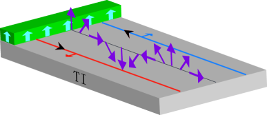
Figure 1: (Color online) Illustration of charge and spin interference patterns between two counter-propagating helical waves. The gray block is a 3DTI with a magnetic edge impurity (green stripe) lying along the $x$-axis on the surface. An incident helical wave along $y$-direction with spin polarized in the $x$-direction (blue line) is backscattered by the magnetic edge and the spin is flipped (red line). The interference of the two orthogonal helical waves leads to a constant LDOS in the charge channel, but a spiral LDOS in the spin channel (purple arrows) in the $yz$-plane.

With the presence of TRS, the backscattering by nonmagnetic impurities is known to be forbidden on the surface of 3DTIs, due to the $\pi$ Berry’s phase associated with the full rotation of electron spin. Ando1998 ; Qi2010 In experiments, this manifests in the invisibility of the scattering wave vector $2k_{F}$ in FT-STS. Yazdani2009 It would then be interesting to ask how the surface states respond differently to magnetic impurities, and what are their characteristic signatures in STM measurements. With magnetic impurities, naively one would expect to see a nontrivial interference pattern since backscattering is allowed due to the breaking of TRS. However, it turns out that the Friedel oscillation in the charge LDOS, which is measured in an ordinary STM experiment with a nonmagnetic tip, is still suppressed in the same way as nonmagnetic impurities. The broken TRS would only manifest itself in the spin LDOS measured by a spin-polarized STM tip. Liu2009

To understand this result, we first present a simple picture of the interference between two counter-propagating helical waves on the surface of a 3DTI, and then give a complete theoretical survey in the next section. Consider a magnetic edge impurity placed along the $x$-axis on the surface. For the effective Hamiltonian $H_{0}=\hbar v_{F}\hat{z}\cdot(\mbox{\boldmath$\sigma$}\times{\bf k})$, the electron state propagating along $y$ direction perpendicular to the impurity line has spin polarized to $x$-direction, with the wavefunction $\psi_{1}=\frac{1}{\sqrt{2}}e^{ik_{F}y}(1\;1)^{\text{T}}$. Here the superscript “T” indicates the transpose. This wave is then backscattered by the magnetic edge and counter-propagates in $-y$-direction. For the same energy, the state with opposite ${\bf k}$ must have opposite spin, with the wavefunction $\psi_{2}=\frac{1}{\sqrt{2}}e^{-ik_{F}y}(-1\;1)^{\text{T}}$. This situation is illustrated in Fig.1. A simple calculation shows that the interference of the two counter-propagating helical waves, $\psi(y)=\frac{1}{\sqrt{2}}(\psi_{1}(y)+\psi_{2}(y))$, leads to a constant charge LDOS on the surface $\left\langle\rho\right\rangle_{\psi}=|\psi^{\dagger}\psi(y)|=1$ since $\psi_{1}$ and $\psi_{2}$ have orthogonal spin. However the interference leads to a spiral spin LDOS in $yz$-plane as $\langle{\bf s}\rangle_{\psi}=\psi^{\dagger}{\bf s}\psi=[0,-\frac{\hbar}{4}\sin(2k_{F}y),-\frac{\hbar}{4}\cos(2k_{F}y)]$, where ${\bf s}=\frac{\hbar}{2}\mbox{\boldmath$\sigma$}$ is the electron spin operator. Therefore a STM experiment with a nonmagnetic tip will observe no interference pattern while one with a magnetic tip will observe the oscillation of the spin density of states. Such a contrast between charge and spin density of states is a unique signature of the helical liquid, which is a direct demonstration of the locking between spin and momentum.

To observe such a spin interference pattern, a more convenient setup is a closed “magnetic wall” as shown in Fig.2. Consider a magnetic layer deposited everywhere on the 3DTI surface except a hole in the middle with the disk shape. The magnetic layer can open a gap on the surface state, such that the low energy surface states are trapped in the hole region and form standing wave. Similar to the straight line magnetic impurity discussed above, the standing wave trapped by the magnetic barrier can be obtained by setting the boundary condition of fixed spin at the boundary of the hole. For large $R$ ($R\gg 1/k_{F}$) the spin density of the standing wave has the behavior of $\langle s_{R}\rangle\sim\frac{\sin(2k_{F}R)}{\sqrt{R}}$, $\langle s_{z}\rangle\sim\frac{\cos(2k_{F}R)}{\sqrt{R}}$, with $R$ and $z$ standing for longitudinal and perpendicular directions in a spherical coordinate. A unique property of the helical surface states is the spin-charge lockingraghu2010 . For the effective Hamiltonian $H_{0}=\hbar v_{F}\hat{z}\cdot(\mbox{\boldmath$\sigma$}\times{\bf k})$, the electric current operator in the long wavelength limit is ${\bf j}=\nabla_{\bf k}H_{0}=\hbar v_{F}\hat{z}\times\mbox{\boldmath$\sigma$}$. Therefore there is a loop charge current $j_{\phi}=-2ev_{F}\langle s_{R}\rangle$ along the azimuthal direction associated with the spin density.

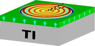
Figure 2: (Color online) Standing wave of spin interference between two helical waves inside a closed “magnetic wall” on top of a 3DTI surface. The magnetic wall is surrounded by a magnetic layer deposited on top of the 3DTI surface, which opens a gap in the helical surface states and plays the role of a barrier. The out-of-plane spin LDOS is exhibited by the colored rings, and the in-plane spin LDOS is indicated by the dark arrows.

III General formulation of Stationary phase approximation approach to QPI on the surface of 3DTI

In this section, we obtain the general long-distance features of charge and spin LDOS on the surface of a generic 3DTI induced by nonmagnetic and magnetic impurities using the stationary phase approximation method. Ruth1966 We study both point-like and edge-like impurities. We shall focus first on the behavior of a special kind of CEC where the stationary points are extremal points, and then generalize our results to generic CEC with higher order nesting points.

III.1 Point impurity

We start by considering a point defect on the surface of a 3DTI. The Hamiltonian with a single impurity is

$$H=\int d^{2}{\bf r}\psi^{\dagger}({\bf r})\left[h_{0}({\bf k})+V\sigma^{\mu}\delta({\bf r})\right]\psi({\bf r}),$$ (1)

where $\sigma^{\mu}=1$ for $\mu=0$ and $\sigma^{a}=\sigma^{x,y,z}$ is the Pauli matrices for $a=1,2,3$. ${\bf k}=-i\nabla$ is the momentum operator. For such a potential the LDOS can be expressed exactly. Using the $\sigma^{\mu}$ matrices, the charge and spin LDOS are combined to the form

$$\rho_{\nu}(\omega,{\bf R})=-\frac{1}{\pi}{\rm Im}\{{\rm tr}\left[G^{r}(\omega,{\bf R},{\bf R})\sigma^{\nu}\right]\},$$ (2)

with $G^{r}(\omega,{\bf R},{\bf R^{\prime}})$ being the retarded Green’s function in real space. Let $\rho_{\nu 0}(\omega)$ be the LDOS of the unperturbed system with $V=0$, the deviation of the LDOS from the background value $\rho_{\nu 0}(\omega)$ is then given by

$$\delta\rho_{\mu\nu}(\omega,{\bf R}) \equiv \rho_{\nu}(\omega,{\bf R})-\rho_{\nu 0}(\omega)$$ (3)

$$= -\frac{1}{\pi}\text{Im}\int\frac{d^{2}kd^{2}k^{\prime}}{(2\pi)^{4}}e^{i({\bf k-k^{\prime}})\cdot{\bf R}}\times$$

$$\text{tr}\left[{G}^{r}_{0}(\omega,{\bf k})T^{\mu}(\omega,{\bf k},{\bf k}^{\prime}){G}^{r}_{0}(\omega,{\bf k^{\prime}})\sigma^{\nu}\right].$$

Here $G^{r}_{0}(\omega,{\bf k})$ is the free retarded Green’s function governing the CEC under consideration. For the topological surface states $G^{r}_{0}(\omega,{\bf k})=(\omega+i\delta-h_{0}({\bf k}))^{-1}$. The T-matrix $T^{\mu}(\omega,{\bf k,k^{\prime}})$ is defined by

$$T^{\mu}(\omega)=V\sigma^{\mu}\left[1-V\sigma^{\mu}G^{r}_{0}(\omega)\right]^{-1},$$ (4)

which is momentum independent when the impurity has a $\delta$-function potential, and we have denoted the real space Green’s function $G^{r}_{0}(\omega)=\int\frac{d^{2}k}{(2\pi)^{2}}{G}^{r}_{0}(\omega,{\bf k})$. As is required by the TRS, $G_{0}^{r}(\omega)$ is always proportional to the identity matrix.

We first note that the spin LDOS induced by a nonmagnetic impurity vanishes uniformly, i.e., $\delta\rho_{0a}\equiv 0$ for $a=1,2,3$. This is a direct consequence of TRS, because under time-reversal transformation $\Theta=i\sigma^{y}$, we have $\Theta^{-1}\sigma^{a}\Theta=-\sigma^{a^{\text{T}}}$ and $\Theta^{-1}G^{r}_{0,k}\Theta=G_{0,-k}^{r^{\text{T}}}$, then the trace in Eq.(3) satisfies $\text{tr}[G^{r}_{0,k}T^{0}G^{r}_{0,k^{\prime}}\sigma^{a}]=-\text{tr}[G^{r}_{0,-k^{\prime}}T^{0}G^{r}_{0,-k}\sigma^{a}]$, where we have abbreviated $G^{r}_{0}(\omega,{\bf k})\equiv G^{r}_{0,k}$. By interchanging ${\bf k}$ and $-{\bf k}^{\prime}$ in the integral in Eq.(3), one is led to the result $\delta\rho_{0a}(\omega,{\bf R})=0$. To obtain other components of the T-matrix, we expand the T-matrix into a spin-dependent and spin-independent parts as

$$T^{a} = T^{a}_{a}\sigma^{a}+T^{a}_{0}$$

$$T^{a}_{a} = \frac{V}{1-V^{2}G^{r2}_{0}(\omega)},~{}T^{a}_{0}=\frac{V^{2}G^{r}_{0}(\omega)}{1-V^{2}G^{r2}_{0}(\omega)}$$

$$T^{0} = \frac{V}{1-VG^{r}_{0}(\omega)}$$ (5)

where the fact that $G^{r}_{0}(\omega)$ is proportional to identity has been used, and no summation over repeated indices is implied throughout the paper. Similar to the argument in $\delta\rho_{0a}$ case, we see that the contribution of $T^{a}_{a}$ to the charge LDOS of a magnetic impurity $\delta\rho_{a0}$ vanishes. Hence we have $\delta\rho_{a0}/\delta\rho_{00}=T_{0}^{a}/T^{0}$. Therefore, in the following, we shall focus only on $\delta\rho_{00}$ and $\delta\rho_{ab}$.

To proceed, the measured LDOS in Eq.(3) is then rewritten in the diagonal basis of the topological surface bands. Define the unitary matrices $U_{\bf k}$ such that $U_{\bf k}^{\dagger}h_{0}({\bf k})U_{{\bf k}}$ diagonalizes $h_{0}({\bf k})$, Eq.(3) becomes

$$\delta\rho_{\mu\nu}(\omega,{\bf R})= -\frac{1}{\pi}\text{Im}\int\frac{d^{2}kd^{2}k^{\prime}}{(2\pi)^{4}}e^{i({\bf k-k^{\prime}})\cdot{\bf R}}\text{tr}\left[(U^{\dagger}_{k}G^{r}_{0,k}U_{k})\right.$$ (6)

$$\left.(U^{\dagger}_{k}T^{\mu}U_{k^{\prime}})(U^{\dagger}_{k^{\prime}}G^{r}_{0,k^{\prime}}U_{k^{\prime}})(U^{\dagger}_{k^{\prime}}\sigma^{\nu}U_{k})\right]$$

$$= -\frac{1}{\pi}\text{Im}\int\frac{d^{2}kd^{2}k^{\prime}}{(2\pi)^{4}}e^{i({\bf k-k^{\prime}})\cdot{\bf R}}\times$$ (7)

$$\sum_{nm}\frac{\gamma^{\mu\nu}_{nm}({\bf k},{\bf k}^{\prime})\Sigma^{\nu^{\ast}}_{nm}({\bf k},{\bf k}^{\prime})}{(\omega+i\delta-\varepsilon_{n})(\omega+i\delta-\varepsilon_{m}^{\prime})},$$

where $\varepsilon_{n(m)}({\bf k})$ are the energy eigenvalues of the bands $|n(m){\bf k}\rangle$, and we have defined $\Sigma^{\mu}_{nm}({\bf k,k^{\prime}})=\langle n{\bf k}|\sigma^{\mu}|m{\bf k^{\prime}}\rangle$, as well as

$$\gamma^{\mu\nu}_{nm}({\bf k},{\bf k}^{\prime})=\left\{\begin{array}[]{cc}T^{0}\Sigma^{0}_{nm},\;\;\;\;\;\;\;\;\;\;\;\;\;\;\mu=\nu=0,\\ T^{a}_{a}\Sigma^{a}_{nm}+T^{a}_{0}\Sigma^{0}_{nm},\;\mu=a,\nu=b.\end{array}\right.$$ (10)

Following the standard process of density of states calculations, Ruth1966 the integrations over ${\bf k}$ and ${\bf k}^{\prime}$ are then converted into coordinates $d{\bf k}=(dk_{\bot},dk_{\phi})$ as

$$\delta\rho_{\mu\nu}(\omega,{\bf R})= - \frac{1}{\pi}{\text{I}m}\oint\frac{dk_{\phi}dk_{\phi}^{\prime}e^{i({\bf k-k^{\prime}})\cdot{\bf R}}}{(2\pi)^{4}}\int\frac{d\varepsilon_{n}d\varepsilon_{m}^{\prime}}{|\nabla_{\bot}\varepsilon_{n}\nabla^{\prime}_{\bot}\varepsilon_{m}^{\prime}|}$$ (11)

$$\times \sum_{nm}\frac{\gamma^{\mu\nu}_{nm}({\bf k},{\bf k}^{\prime})\Sigma^{\nu^{\ast}}_{nm}({\bf k},{\bf k}^{\prime})}{(\omega+i\delta-\varepsilon_{n})(\omega+i\delta-\varepsilon_{m}^{\prime})},$$

where $k_{\bot}$ and $k_{\phi}$ are components of ${\bf k}$ normal and tangential to the CEC, respectively.

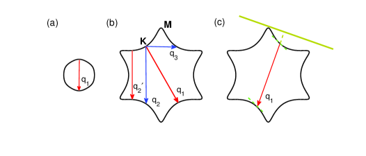
Figure 3: (Color online) Schematic picture of CEC and stationary points for point and edge impurities. (a) Convex CEC where there is only one pair of stationary points connected by the red arrow along any given direction for both point and line impurities. (b) Concave CEC for point impurity where there are multiple pairs of stationary points. Nonstationary points are shown for example as blue arrows. (c) Concave CEC for edge impurities (brown line) where the slopes (green dashed lines) at the pair of stationary points are the same.

To evaluate the loop integrals along the CEC, it is essential to introduce the stationary phase approximation. For example, consider the LDOS at a point ${\bf R}=R\hat{y}$ (here and hereafter we shall always take the $y$-direction for example), the phase factor $e^{i{\bf(k-k^{\prime})\cdot R}}=e^{i(k_{y}-k_{y}^{\prime})R}$. Locally, one can write $k_{y}=k_{y}(\varepsilon,k_{x})$ as a function of energy $\varepsilon$ and $k_{x}$. For large distance $R$ from the impurity, the phase factors $e^{ik_{y}(\varepsilon,k_{x})R}$ and $e^{-ik_{y}^{\prime}(\varepsilon^{\prime},k_{x}^{\prime})R}$ vary rapidly with respect to $k_{x}$ and $k_{x}^{\prime}$ for almost every point on the CEC, so that most of the integrations cancel out exactly except for the stationary points, ${\bf k}_{i}$, Ruth1966 which satisfy the condition

$$\frac{\partial k_{y}(\varepsilon,k_{x})}{\partial k_{x}}=\frac{\partial k_{y}^{\prime}(\varepsilon^{\prime},k_{x}^{\prime})}{\partial k_{x}^{\prime}}=0.$$ (12)

The stationary points defined above include i) extremal points such as the pairs connected by ${\bf q}_{1}$ in Figs.3(a) and (b), where the second derivative $\partial^{2}k_{y}/\partial k_{x}^{2}$ is nonvanished; ii) the turning points such as the pair connected by ${\bf q}_{2}^{\prime}$ in Fig.3(b), where the second derivative also vanishes. In the following, we first focus only on the extremal points, and leave the more general discussions to Sect.III.3.

Having identified the pairs of stationary points on the CEC in direction ${\bf R}$, the loop integrals in Eq.(11) at large distances are then approximated by the summation of integrals in the neighborhood of all the stationary-point pairs, which is the essence of the method of the stationary phase approximation. To start with, we first change the integral variables as $d^{2}k=d\varepsilon dk_{x}/\hbar|v_{yi}|$, where $v_{yi}=\partial\varepsilon({\bf k})/\hbar\partial k_{yi}$, and then expand the CEC at the extremal points as $k_{y}=k_{yi}-(k_{x}-k_{xi})^{2}/2\rho_{xi}$, where $\rho_{xi}=-[\partial^{2}k_{yi}(\varepsilon,k_{x})/\partial^{2}k_{xi}]^{-1}$ is the principle radii of curvature of the CEC at the extremal points, which is positive for maxima while negative for minima. Under this approximation, Eq.(11) becomes

$$\delta\rho_{\mu\nu}(\omega,{\bf R})\simeq -\frac{1}{\pi}\text{Im}\sum_{mn}\sum_{ij}\int\frac{d\varepsilon_{n}}{(2\pi)^{2}}\frac{1}{\omega+i\delta-\varepsilon_{n}}\frac{e^{ik_{yi}R}}{\hbar|v_{yi}|}$$ (13)

$$\times\int\frac{d\varepsilon_{m}^{\prime}}{(2\pi)^{2}}\frac{1}{\omega+i\delta-\varepsilon_{m}^{\prime}}\frac{e^{-ik_{yj}^{\prime}R}}{\hbar|v_{yj}^{\prime}|}$$

$$\times\int_{-\infty}^{\infty}dx\;e^{-i\frac{x^{2}}{2\rho_{xi}}R}\int_{-\infty}^{\infty}dx^{\prime}\;e^{i\frac{x^{{\prime}^{2}}}{2\rho_{xj}^{\prime}}R}$$

$$\times\gamma^{\mu\nu}_{nm}({\bf k},{\bf k}^{\prime})\Sigma^{\nu^{\ast}}_{nm}({\bf k},{\bf k}^{\prime}),$$

where we have denoted $x=k_{x}-k_{xi}$, $x^{\prime}=k_{x}^{\prime}-k_{xj}^{\prime}$, and all the quantities at the extremal points ($ij$) still depend on the energies $\varepsilon$ and $\varepsilon^{\prime}$. Now the matrix element $\Sigma^{\mu}_{nm}({\bf k},{\bf k}^{\prime})$ at the extremal points is in general some nonzero constant $C^{\mu}_{ni,mj}(\varepsilon,\varepsilon^{\prime})$, except that it vanishes when $\mu=0$ and the pair of stationary points are time-reversal partners $|n{\bf k}_{i}\rangle=\Theta\hat{K}|m{\bf k}^{\prime}_{j}\rangle$. Here $\hat{K}$ is the complex conjugation operator. Examples are shown as the pairs of stationary points connected by ${\bf q}_{1}$’s in Figs.3(a) and (b) for convex and concave CEC respectively. To obtain the generic behavior of the interference pattern, the matrix element is expanded in the distance $x,x^{\prime}$ to the stationary points as $\Sigma^{\mu}_{nm}(x,x^{\prime})=C^{\mu}_{ni,mj}+ax+a^{\prime}x^{\prime}+o(x)+o(x^{\prime})$, where $C^{\mu}_{ni,mj}=0$ for $\mu=0$ at TRP, and a nonvanishing but energy dependent constant otherwise. Inserting the series into Eq.(13), one can integrate first over $x$ and $x^{\prime}$ by using the relations $\int_{-\infty}^{\infty}dxe^{iCx^{2}}=\sqrt{\pi/|C|}e^{i\frac{\pi}{4}\text{sgn}(C)}$ and $\int_{-\infty}^{\infty}dxx^{2}e^{iCx^{2}}=\sqrt{\pi}/(2|C|^{3/2})e^{-i\frac{\pi}{4}\text{sgn}(C)}$, and then integrate over the energies using the residue theorem by summation over the integrand at the poles $\varepsilon=\varepsilon^{\prime}=\omega+i\delta$. Finally by taking the limit $\omega=\varepsilon_{F}$, $\delta\rightarrow 0^{+}$ we get

$$\delta\rho_{\mu\nu}(\omega,{\bf R}) \simeq \frac{1}{2\pi^{2}\hbar^{2}R}\text{Im}\sum_{mn}\sum_{ij}e^{i(k_{yi}-k_{yj}^{\prime})R}\frac{|\rho_{xi}\rho_{xj}^{\prime}|^{\frac{1}{2}}}{|v_{yi}v_{yj}^{\prime}|}$$

$$\times [e^{i(\phi_{i}-\phi_{j}^{\prime})}\sum_{s}T^{\mu}_{s}C^{s}_{ni,mj}C^{\nu^{\ast}}_{ni,mj}+\frac{1}{R}$$

$$\times ({a^{\prime}}^{2}e^{i(\phi_{i}+\phi_{j}^{\prime})}\left|\rho_{xj}^{\prime}\right|+a^{2}e^{-i(\phi_{i}+\phi_{j}^{\prime})}\left|\rho_{xi}\right|)]_{\varepsilon_{F}}$$

where $\phi_{i}=-\frac{\pi}{4}\text{sgn}(\rho_{xi})$. This is the long wavelength behavior of LDOS induced by a point impurity. In the above result, we have $s=0$ and $T^{0}_{0}\equiv T^{0}=V/(1-VG^{r}_{0}(\omega))$ for the charge LDOS of a nonmagnetic impurity $\delta\rho_{00}$. While for the spin LDOS of a magnetic impurity $\delta\rho_{ab}$, the summation is over $s=a,0$, where $T^{a}_{a}$ and $T^{a}_{0}$ are respectively the spin-dependent and spin-independent coefficients in the T-matrix expansion introduced above.

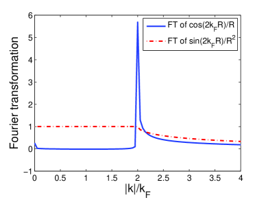
Figure 4: (Color online) Fourier transformation of the LDOS with $R^{-1}$ and $R^{-2}$ power laws.

There are several comments regarding this result. Firstly, for a pair of non-TRS stationary points like ${\bf q}_{2}$ in Fig.3(b), the leading power is given by the first term in Eq.(LABEL:pointfinal), which is of $R^{-1}$. While for a pair of TRS stationary points as ${\bf q}_{1}$ in Figs.3 (a) and (b), the first nonvanishing contribution to the power law is dominated by the second term in Eq.(LABEL:pointfinal) as $R^{-2}$ for nonmagnetic impurity, and for magnetic impurity with ordinary tip. Such suppression of LDOS is a direct consequence of the absence of backscattering of helical waves due to TRS. Correspondingly in the fourier transform of LDOS, there is a sharp peak at $k=2k_{F}$ for $R^{-1}$ power law, which is absent for $R^{-2}$ power law, as shown in Fig.4. For magnetic impurities with spin-polarized tip, the first term in Eq.(LABEL:pointfinal) dominates no matter whether the pair of stationary points is TRS or not (due to the contribution of the $s=a$ term), which gives the visibility of the TRS scattering wave vector ${\bf q}_{1}$. This distinct response of surface states to magnetic impurities from that of nonmagnetic impurities provides a crucial criteria for the breaking of TRS on the surface of TIs. Xue2009 Secondly, in the discussion above we have assumed the matrix element $\Sigma^{\mu}_{nm}$ to be nonzero if it is not forbidden by time-reversal symmetry. There may be some other reasons for the matrix element to vanish. For example, the states at two TRS stationary points have opposite spin. If the impurity spin happens to be parallel (or anti-parallel) to their spin, the matrix element $\Sigma_{nm}^{\mu}$ can vanish. For non-TRS stationary points, this may occur accidentally, but generically the spin of the two states $n$ and $m$ are not parallel, so that the matrix element is nonvanished for any impurity spin. Since such zeros of matrix elements are at most only realized for some particular directions of the impurity spin, in the following we will focus on the generic cases with nonzero matrix element as long as it is not forbidden by time-reversal symmetry. Thirdly, in the integral over energy, we have assumed $v_{yi},v_{yj}^{\prime}\neq 0$ so that the only poles in the complex energy plane are $\varepsilon=\varepsilon^{\prime}=\omega+i\delta$. However, in general, it is possible that there are other poles from $v_{yi}=0$ or $v_{yj}^{\prime}=0$, which means the stationary points in CEC are also saddle points in the energy-momentum dispersion. In that case, we shall further expand $v_{yi}$ (or $v_{yj}^{\prime}$) around $\omega$ as $v_{yi}(\varepsilon)=v_{yi}(\omega)+(\partial v_{yi}/\partial\varepsilon)(\varepsilon-\omega)+\cdots$, and keep the first nonzero term. This won’t modify the power laws in spatial dependence. Finally, note that when summation over the stationary-point pairs, $(ij)$, we always choose the pair such that one point has positive velocity $v_{yi}$ and the other has negative velocity $v_{yj}^{\prime}$. As a summary of the discussion above, the power laws of LDOS for point impurity are concluded in Table. 1.

Table 1: Power laws of Friedel oscillations for point impurity

  charge LDOS spin LDOS nonmagnetic TRP $R^{-2}$ - non-TRP $R^{-1}$ - magnetic TRP $R^{-2}$ $R^{-1}$ non-TRP $R^{-1}$ $R^{-1}$  

To provide further intuition on the result (LABEL:pointfinal), we consider some simple examples. The first example is a 2DES without spin-orbit coupling described by the familiar Hamiltonian $H_{Q}=\hbar^{2}k^{2}/2m$, which has two degenerate and isotropic Fermi surfaces, as shown in Fig.5(a). According to our theory, the main contribution to the LDOS in this example comes from the intraband scattering of the same spin orientation between two extremal points, which we denote as ‘1’ and ‘2’. At these points we have $k_{y2}=\rho_{x2}=k_{\varepsilon}$, $k_{y1}^{\prime}=\rho_{x1}^{\prime}=-k_{\varepsilon^{\prime}}$, $k_{\varepsilon}=(2m\varepsilon/\hbar^{2})^{1/2}$, $v_{y2}=\hbar k_{y2}/m$, $v_{y1}^{\prime}=\hbar k_{y1}^{\prime}/m$, and $C^{0}_{11}=C^{0}_{22}=1$. Inserting these quantities into Eq.(LABEL:pointfinal) and keeping only to the first order expansion of T-matrix, we get $\delta\rho^{(1)}_{00}(\omega,R\hat{y})\simeq-(Vm^{2}/\pi^{2}\hbar^{4}q)\cos(2qR)/R$, which has $R^{-1}$ power law. Note that the interband contribution to the LDOS in this example is from a pair of TRS extremal points, which has a $R^{-2}$ power law. In contrast, in the example of a 2D Dirac CEC, $H_{D}=\gamma\hat{z}\cdot(\mbox{\boldmath$\sigma$}\times{\bf k})$, there is only one non-degenerate band at a given energy due to the spin splitting, as shown in Fig.5(b). Thus only intraband scattering between a pair of extremal TRP contributes to the LDOS, and $C^{0}_{ni,mj}=0$. Inserting the quantities $k_{y2}=\rho_{x2}=\varepsilon/\gamma$, $k_{y1}^{\prime}=\rho_{x1}^{\prime}=-\varepsilon/\gamma$, and $v_{y1(2)}=\gamma\text{sgn}[k_{y1(2)}]/\hbar$ into Eq.(LABEL:pointfinal), we get $\delta\rho^{(1)}_{00}(\omega,R\hat{y})\simeq(V/4\pi^{2}\gamma^{2})\sin(2qR)/R^{2}$, which is consistent with our expectation.

In a recent STM measurement of the TI Bi₂Te₃ doped with Ag,Xue2009 clear standing waves and scattering wave vectors are imaged through FT-STS when the Fermi surface is of hexagram shape. It is observed that the high intensity regions are always along the $\bar{\Gamma}$-$\bar{M}$ direction, but the intensity in $\bar{\Gamma}$-$\bar{K}$ direction vanishes. This observation can be well-understood using our stationary phase approximation theory. Among the wave vectors ${\bf q}_{1}$, ${\bf q}_{2}$, ${\bf q}_{2}^{\prime}$ and ${\bf q}_{3}$ shown in Fig.3(b), ${\bf q}_{1}$ and ${\bf q}_{2}^{\prime}$ correspond to scattering between stationary points, while ${\bf q}_{3}$ and ${\bf q}_{2}$ do not. This explains why no standing waves corresponding to ${\bf q}_{3}$ are observed in FT-STS. Within the other two, stationary points connected by ${\bf q}_{1}$ are also TRP which shall contribute the power law of $R^{-2}$ according to our result. Therefore its intensity in FT-STS is too weak to be observed. For wave vectors ${\bf q}_{2}$ and ${\bf q}_{2}^{\prime}$ along $\bar{\Gamma}$-$\bar{M}$ direction, ${\bf q}_{2}^{\prime}$ is stationary but non-TRS. Our result shows that this wave vector contributes an $R^{-1}$ power law, which is responsible for the high intensity reported in Ref.Xue2009 .

III.2 Edge impurity

Beside point impurities, one-dimensional line defect in the form of step edge has also been observed on the surface of 3DTI. Manoharan2009 ; Alpichshev2009 Magnetic edge defects can possibly be realized by depositing a magnetic layer on top of a 3DTI. In this section, we discuss the interference patterns of electronic waves induced by magnetic and nonmagnetic edge defects.

We consider an edge defect along the $x$-direction on top of a 3DTI surface with the Hamiltonian $V({\bf r})=V\delta(y)\sigma^{\mu}$. A magnetic edge defect has been illustrated in Fig.1. The main difference between an edge defect and a point defect is the momentum conservation along the edge impurity orientation, which means one of the loop integrations in Eq.(11) should be removed. Following similar calculations as performed in the case of a point impurity, the LDOS for the edge impurity is given by

$$\delta\rho_{\mu\nu}(\omega,{\bf R})= - \frac{1}{\pi}\text{Im}\int\frac{d^{2}kd^{2}k^{\prime}}{(2\pi)^{4}}\delta_{k_{x},k_{x}^{\prime}}e^{i({\bf k-k^{\prime}})\cdot{\bf R}}$$ (15)

$$\times \text{tr}\left[{G}^{r}_{0}(\omega,{\bf k})T^{\mu}(\omega,k_{x}){G}^{r}_{0}(\omega,{\bf k^{\prime}})\sigma^{\nu}\right],$$

where $T^{\mu}(\omega,k_{x})=V\sigma^{\mu}/(1-V\sigma^{\mu}G^{r}_{0}(\omega,k_{x}))$ with $G^{r}_{0}(\omega,k_{x})=\int\frac{dk_{y}}{2\pi}G^{r}_{0}(\omega,{\bf k})$. Similarly as the case of a magnetic point impurity, the T-matrix for a magnetic edge impurity can again be separated into a spin-dependent and a spin-independent terms. However, in the following discussion, we shall keep only to the first order expansion of the T-matrix, $V\sigma^{\mu}$, which is spin-dependent. This simplification is appropriate for weak impurity potential, and it won’t affect the qualitative conclusion of the Friedel oscillation power laws, as we have learned from the case of point impurities.

In the presence of edge impurity, we are usually interested in the LDOS in the direction perpendicular to the edge orientation. Similarly as the case of point impurity, the LDOS in eq.(15) is first transformed into the diagonal basis of the topological surface bands, and then converted into integrations over normal and tangential components as in Eq.(11). By using the stationary phase approximation, now the main contribution to the loop integrals comes from such stationary points where their momentum transfer ${\bf q}$ is normal to the edge orientation, and the “slopes” of CEC at the two stationary points are the same:

$$\frac{\partial}{\partial k_{x}}\left[k_{y}(\varepsilon,k_{x})-k_{y}^{\prime}(\varepsilon^{\prime},k_{x})\right]=0.$$ (16)

Compared with the stationary-point condition for point impurity, the condition for edge impurity allows more possibilities. One such example is shown schematically as ${\bf q}_{1}$ in Fig.3(c) where the pair of stationary points has the same nonvanished slope. Such a pair of scattering end points is not considered as stationary points in the case of point impurities, but are stationary for edge impurities. Following the same logic as the discussion of point impurity in the last section, the CEC is then expanded around the stationary points as $k_{y}=k_{yi}+\alpha_{i}(k_{x}-k_{xi})-(k_{x}-k_{xi})^{2}/2\rho_{xi}$, and the LDOS is approximated by

$$\delta\rho^{(1)}_{\mu\nu}(\omega,{\bf R})\simeq -\frac{V}{\pi}\text{Im}\sum_{mn}\sum_{ij}\int\frac{d\varepsilon_{n}}{(2\pi)^{2}}\frac{1}{\omega+i\delta-\varepsilon_{n}}\frac{e^{ik_{yi}R}}{\hbar|v_{yi}|}\int\frac{d\varepsilon_{m}^{\prime}}{(2\pi)^{2}}\frac{1}{\omega+i\delta-\varepsilon_{m}^{\prime}}\frac{e^{-ik_{yj}^{\prime}R}}{\hbar|v_{yj}^{\prime}|}$$ (17)

$$\times\int_{-\infty}^{\infty}dxe^{-i\frac{x^{2}}{2\rho_{xi}}R}\int_{-\infty}^{\infty}dx^{\prime}e^{i\frac{x^{{\prime}^{2}}}{2\rho_{xj}^{\prime}}R}e^{i\alpha_{i}(x-x^{\prime})}\delta_{x,x^{\prime}}\left[C^{\mu}_{ni,mj}C^{\nu^{\ast}}_{ni,mj}+(ax+a^{\prime}x^{\prime})^{2}\right].$$

Although Eq.(17) looks similar to Eq.(13) in point impurity case, the definition of stationary points for edge impurity in Eq.(16) is quite different from that of point impurity. Therefore, a lot more terms should be included in the summation of stationary-point pairs $(ij)$ here compared with the point impurity case. By integrating out $x(x^{\prime})$ and energy variables, we get

$$\delta\rho^{(1)}_{\mu\nu}(\omega,{\bf R}) \simeq \frac{V}{(2\pi)^{2}\hbar^{2}}\sqrt{\frac{2}{\pi R}}\text{Im}\sum_{mn}\sum_{ij}\frac{|P_{ij}|^{1/2}}{|v_{yi}v_{yj}^{\prime}|}$$ (18)

$$\times e^{i(k_{yi}-k_{yj}^{\prime})R}\left[C^{\mu}_{ni,mj}C^{\nu^{\ast}}_{ni,mj}e^{i\Phi_{ij}}\right.$$

$$+ \left.e^{-i\Phi_{ij}}(a+a^{\prime})^{2}P_{ij}/R\right]_{\varepsilon_{F}},$$

where $P_{ij}=\rho_{xi}\rho_{xj}^{\prime}/(\rho_{xj}^{\prime}-\rho_{xi})$ and $\Phi_{ij}=-\frac{\pi}{4}\text{sgn}(P_{ij})$. In the equation above we have assumed $v_{yi},v_{yj}^{\prime}\neq 0$ and $\rho_{xi}\neq\rho_{xj}^{\prime}$. In other words, this result is not applicable to the case where the CEC near the pair of stationary points is nested to the second order expansion. If such nesting happens, the quadratic terms in the expansion of CEC near the stationary points cancel out exactly, and higher orders expansion should be employed. The power laws of Friedel oscillations for edge impurity are summarized in Table. 2, which shall be used to explain the STM measurements about edge impurities. Manoharan2009 ; Alpichshev2009

Table 2: Power laws of Friedel oscillations for edge impurity

  ordinary spin polarized nonmagnetic TRP $R^{-3/2}$ - non-TRP $R^{-1/2}$ - magnetic TRP $R^{-3/2}$ $R^{-1/2}$ non-TRP $R^{-1/2}$ $R^{-1/2}$  

To have a feeling of how Eq.(18) works explicitly, again we apply it to the examples of 2DEG Hamiltonian $H_{Q}$ and 2D Dirac Hamiltonian $H_{D}$ discussed previously. A few lines of calculations yield that for 2D quadratic dispersion, $\delta\rho_{00}^{(1)}(\omega,R\hat{y})=(Vm^{2}/2\pi^{2}\hbar^{4}q^{3/2})\sin(2qR-\frac{\pi}{4})/\sqrt{\pi R}$, which is consistent with the experimental observation in 2DEG.Crommie1993 For 2D Dirac fermion, $\delta\rho_{00}^{(1)}(\omega,R\hat{y})=(V/8\pi^{2}\gamma^{2}\sqrt{\pi q})\sin(2qR+\frac{\pi}{4})/R^{3/2}$, which is a consequence of the absence of backscattering in helical liquid. Information in reciprocal space can be extracted via FT-STS similarly to the point-impurity case exhibited in Fig.4, where a notable sharp peak is present at $k=2k_{F}$ for a 2DEG, but is absent for the helical liquid.

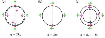
Figure 5: (Color online) Schematic CEC of (a) quadratic, (b) Dirac, and (c) Rashba dispersions. The spin orientations for each degenerate band are indicated respectively by the green (solid) and purple (dotted) arrows. The stationary points are represented by red and blue dots, which are connected by the scattering vector ${\bf q}$ shown as dashed arrows. The intraband scattering occurs between the stationary points with the same color, while the interband scattering occurs between those with different colors.

In an experiment by Gomes et al., a nonmagnetic step is imaged by STM topography in Sb $(111)$ surface. Manoharan2009 The Fermi surface consists of one electron pocket at $\bar{\Gamma}$ surrounded by six hole pockets in $\bar{\Gamma}$-$\bar{M}$ direction, where the surface dispersion has a Rashba spin splitting. The measured LDOS in $\bar{\Gamma}$-$\bar{M}$ direction is fitted by a single $q$-parameter using the zeroth-order of Bessel function of the first kind, see Fig.2(c) in Ref.Manoharan2009 , which agrees exactly with our result in Table. 2. Along $\bar{\Gamma}$-$\bar{M}$ direction, the surface band can be modeled by a Rashba Hamiltonian where the LDOS is dominated by interband scattering between a pair of non-TRS stationary points, as shown in Fig.5(c). According to our analysis, the Friedel oscillation has $R^{-1/2}$ power law, which is the asymptotic expansion of $J_{0}(qR)$ at large distances. Another STM experiment studying the edge impurity by Alpichshev et. al. Alpichshev2009 is in Bi₂Te₃ where hexagonal warping effect exists, and a nonmagnetic step defect is observed on crystal surface. A strongly damped oscillation is reported when the bias voltage is at the energy with a convex Fermi surface as shown in Fig.3(a). Though no fitting of the experimental data is estimated in this region, our results predict a $R^{-3/2}$ power law. Pronounced oscillations at higher bias voltages where the hexagon warping effect emerges are observed with $R^{-1}$ fitting. Despite of the quantitative difference with our result of $R^{-1/2}$, this $R^{-1}$ oscillation has been explained in several other works Zhou2009 ; Lee2009 beyond our simple model.

The results summarized in Tables. 1 and 2 provide a quantitative description of the QPI by magnetic impurities in general, which include the interference between two orthogonal helical waves discussed in Sect. II as a particular case. The interference of helical waves corresponds to the scattering between two TRS stationary points, like the ${\bf q}_{1}$’s in Figs. 3(a), (b) and (c). The interesting thing is that the LDOS in charge and spin channels from the very same pair of TRS stationary points have quite distinct behavior. With magnetic impurities, the power laws of charge LDOS are $R^{-2}$ and $R^{-3/2}$ for point and edge impurities respectively. As a result of TRS, the charge LDOS has higher power indices than the $R^{-1}$ and $R^{-1/2}$ modulations of the corresponding spin-polarized LDOS, which manifests the TRS breaking. To distinguish the response of topological surface states to magnetic impurities from that of the nonmagnetic impurities, Xue2009 spin-resolved STM experiments are essential.

III.3 Friedel oscillations for CEC with generic shape

In this section, we generalize the results obtained above and obtain the most general formulation of the QPI on the surface of a 3DTI.

In the discussion of point impurity in Sect.III.1, we have focused on the case of extremal points, around which the expansion of the CEC has nonvanishing second derivatives. However it is in general also possible that the principle radii of the curvature of the CEC at the stationary points, $\rho_{xi}$, diverges so that the third or even higher order expansions of the CEC at the stationary points should be employed. For example, when the stationary points are also turning points on the CEC, see ${\bf{q}}_{2}^{\prime}$ in Fig.3(b), the expansion of the CEC should be kept to the third order. In the case of edge impurity presented in Sect.III.2, it is possible that $\rho_{xi},\rho_{xj}^{\prime}\neq 0$, but $\rho_{xi}=\rho_{xj}^{\prime}$ so that $P_{ij}$ diverges. This happens when the CEC near the stationary points is highly nested, and we need to go beyond the quadratic expansion of the CEC till the first power at which the two segments of the CEC are not nested.

To understand the LDOS behavior in ordinary and spin-resolved STM experiments in these most general situations, we assume in general that the first nonvanishing coefficients in the expansion of the CEC around the stationary points have the order $l$ and $h$ respectively, where $l,h\in{\rm N}$ are generically different. Then $k_{y}(\varepsilon,k_{x})$ and $k_{y}^{\prime}(\varepsilon^{\prime},k_{x}^{\prime})$ on the CEC are expanded around the stationary points separately as $k_{y}=k_{yi}+\beta^{(l)}_{i}(k_{x}-k_{xi})^{l}$ and $k_{y}^{\prime}=k_{yj}^{\prime}+\beta_{j}^{\prime(h)}(k_{x}^{\prime}-k_{xj}^{\prime})^{h}$, where the $\beta$’s are the first nonzero expansion coefficients with $\beta^{(l)}_{i}=(\partial^{l}k_{y}/\partial k_{xi}^{l})/l!$ and similarly for $\beta_{j}^{\prime(h)}$. Notice that in the case of edge impurity, if $l=h$, one more constraint $\beta^{(l)}_{i}\neq\beta_{j}^{\prime(h)}$ should be further imposed on the expansion to obtain a meaningful LDOS. Having analyzed the properties of the stationary points on the CEC, the same calculation procedures as performed in Sects.III.1 and III.2 for point and edge impurities can be carried out in a straightforward way, which leads to the following most general results for point impurity

$$\rho^{(1)}_{\mu\nu}(\omega,{\bf R}) \propto \frac{V}{R^{\frac{1}{l}+\frac{1}{h}}}\text{Im}\sum_{mn}\sum_{ij}\left\{\frac{e^{i(k_{yi}-k_{yj}^{\prime})R}}{|v_{yi}v_{yj}^{\prime}||\beta^{(l)}_{xi}|^{\frac{1}{l}}|\beta^{\prime(h)}_{xj}|^{\frac{1}{h}}}\right.$$ (19)

$$\times \left.\left[C^{\mu}_{ni,mj}C^{\nu^{\ast}}_{ni,mj}+\frac{a^{2}}{|\beta^{(l)}_{xi}|^{\frac{2}{l}}R^{\frac{2}{l}}}+\frac{a^{\prime 2}}{|\beta_{xj}^{\prime(h)}|^{\frac{2}{h}}R^{\frac{2}{h}}}\right]\right\}_{\varepsilon_{F}},$$

and for edge impurity

$$\rho^{(1)}_{\mu\nu}(\omega,{\bf R}) \propto \frac{V}{R^{\frac{1}{\text{max}(l,h)}}}\text{Im}\sum_{mn}\sum_{ij}\left\{\frac{e^{i(k_{yi}-k_{yj}^{\prime})R}}{|v_{yi}v_{yj}^{\prime}|}\right.$$ (20)

$$\times |\beta^{(l)}_{xi}-\beta_{xj}^{\prime(h)}|^{\frac{-1}{\text{max}(l,h)}}\left[C^{\mu}_{ni,mj}C^{\nu^{\ast}}_{ni,mj}\right.$$

$$+ \left.\left.(a+a^{\prime})^{2}\left(R|\beta^{(l)}_{xi}-\beta_{xj}^{\prime(h)}|\right)^{\frac{-2}{\text{max}(l,h)}}\right]\right\}_{\varepsilon_{F}}.$$

These two equations complete the key results in this work. In the above, we have used the notation $\text{min}(l,h)$ and $\text{max}(l,h)$ to represent taking the minimum or the maximum one between $l$ and $h$. The corresponding power laws of the Friedel oscillations in these most general cases are summarized in Tables. 3 and 4. We see that by taking $l=h=2$, these results recover those exhibited in Tables. 1 and 2 obtained in the last two sections.

Table 3: General power laws of Friedel oscillations for point impurity

  ordinary spin-polarized nonmagnetic TRP $R^{-(\frac{1}{l}+\frac{1}{h})-\frac{2}{\text{min}(l,h)}}$ - non-TRP $R^{-(\frac{1}{l}+\frac{1}{h})}$ - magnetic TRP $R^{-(\frac{1}{l}+\frac{1}{h})-\frac{2}{\text{min}(l,h)}}$ $R^{-(\frac{1}{l}+\frac{1}{h})}$ non-TRP $R^{-(\frac{1}{l}+\frac{1}{h})}$ $R^{-(\frac{1}{l}+\frac{1}{h})}$  

Table 4: General power laws of Friedel oscillations for edge impurity

  ordinary spin-polarized nonmagnetic TRP $R^{-\frac{3}{\text{max}(l,h)}}$ - non-TRP $R^{-\frac{1}{\text{max}(l,h)}}$ - magnetic TRP $R^{-\frac{3}{\text{max}(l,h)}}$ $R^{-\frac{1}{\text{max}(l,h)}}$ non-TRP $R^{-\frac{1}{\text{max}(l,h)}}$ $R^{-\frac{1}{\text{max}(l,h)}}$  

IV Conclusions

In conclusion, long-distance asymptotic behavior of the LDOS for nonmagnetic and magnetic, point and edge impurities on a generic shape CEC are derived in Eqs.(LABEL:pointfinal), (18), (19), and (20) using the stationary phase approximation approach. The corresponding power laws of Friedel oscillations are summarized in Tables. 1 to 4. The QPI induced by surface magnetic impurities is studied in particular, to illustrate the fact that the interference patterns of charge intensities are indistinguishable from those of nonmagnetic impurities, while the spin LDOS show distinct behavior from those of nonmagnetic impurities. We propose a closed “magnetic wall” geometry which manifests such a unique interference property of helical liquids. These results depend only on the TRS as well as the local geometry around the stationary points on the CEC, which provide a systematic tool for the analysis of STM experiments for generic surface states.

- (1) X.-L. Qi and S.-C. Zhang, Rev. Mod. Phys. 83, 1057 (2011).
- (2) Hasan, M. Z., and C. L. Kane, Rev. Mod. Phys. 82, 3045 (2010).
- (3) J. E. Moore, Nature 464, 194 (2010).
- (4) H. J. Zhang, C.-X. Liu, X.-L. Qi, X. Dai, Z. Fang, and S.-C. Zhang, Nature Phys. 5, 438 (2009).
- (5) Y. Xia, D. Qian, D. Hsieh, L. Wray, A. Pal, H. Lin, A. Bansil, D. Grauer, Y. S. Hor, R. J. Cava et al., Nat Phys. 5, 398 (2009).
- (6) Y. L. Chen, J. G. Analytis, J.-H. Chu, Z. K. Liu, S.-K. Mo, X.-L. Qi, H. J. Zhang, D. H. Lu, X. Dai, Z. Fang, S.-C. Zhang, I. R. Fisher, Z. Hussain and Z.-X. Shen, Science 325, 178 (2009).
- (7) D. Hsieh, Y. Xia, D. Qian, L. Wray, J. H. Dil, F. Meier, J. Osterwalder, L. Patthey, J. G. Checkelsky, N. P. Ong, A. V. Fedorov, H. Lin, A. Bansil, D. Grauer, Y. S. Hor, R. J. Cava, and M. Z. Hasan, Nature (London) 460, 1101 (2009).
- (8) S. Raghu, S. B. Chung, X.-L. Qi, and S.-C. Zhang, Phys. Rev. Lett. 104, 116401 (2010).
- (9) L. Fu, Phys. Rev. Letts. 103, 266801 (2009).
- (10) J. Friedel, Phil. Mag. 43, 153 (1952).
- (11) T. Zhang, P. Cheng, X. Chen, J.-F. Jia, X. Ma, K. He, L. Wang, H. Zhang, X. Dai, Z. Fang et al., Phys. Rev. Lett. 103, 266803 (2009).
- (12) T. Hanaguri, K. Igarashi, M. Kawamura, H. Takagi, and T. Sasagawa, Phys. Rev. B 82, 081305 (2010).
- (13) Z. Alpichshev, J. G. Analytis, J.-H. Chu, I. R. Fisher, Y. L. Chen, Z. X. Shen, A. Fang, and A. Kapitulnik, Phys. Rev. Lett. 104, 016401 (2010).
- (14) Zhanybek Alpichshev, J. G. Analytis, J.-H. Chu, I. R. Fisher and A. Kapitulnik, Phys. Rev. B 84, 041104(R) (2011)
- (15) Zhanybek Alpichshev, Rudro R. Biswas, Alexander V. Balatsky, James G. Analytis, Jiun-Haw Chu, Ian R. Fisher, Aharon Kapitulnik, e-print arXiv:1108.0022 (2011)
- (16) Haim Beidenkopf, Pedram Roushan, Jungpil Seo, Lindsay Gorman, Ilya Drozdov, Yew San Hor, R. J. Cava, Ali Yazdani, e-print arXiv:1108.2089 (2011)
- (17) Kenjiro K. Gomes, Wonhee Ko, Warren Mar, Yulin Chen, Zhi-Xun Shen, Hari C. Manoharan, arXiv:cond-mat/0909.0921 (unpublished).
- (18) P. Roushan, J. Seo, C. V. Parker, Y. S. Hor, D. Hsieh, D. Qian, A. Richardella, M. Z. Hasan, R. J. Cava, and A. Yazdani, Nature (London) 460, 1106 (2009).
- (19) Jing Wang, Wei Li, Peng Cheng, Canli Song, Tong Zhang,Peng Deng, Xi Chen, Xucun Ma, Ke He, Jin-Feng Jia, Qi-Kun Xue, and Bang-Fen Zhu, Phys. Rev. B 84, 235447 (2011).
- (20) X. Zhou, C. Fang, W.-F. Tsai, and J.P. Hu, Phys. Rev. B 80, 245317 (2009).
- (21) W.-C. Lee, C. Wu, D. P. Arovas, and S.-C. Zhang, Phys. Rev. B 80, 245439 (2009).
- (22) H.-M. Guo, and M. Franz, Phys. Rev. B 81, 041102(R) (2010).
- (23) Rudro R. Biswas, and Alexxander V. Balatsky, e-print arXiv:1005.4780 (unpublished); Phys. Rev. B 81, 233405 (2010), 83, 075439 (2011).
- (24) Q.-H. Wang, D. Wang, and F.-C. Zhang, Phys. Rev. B 81, 035104 (2010).
- (25) M. F. Crommie, C. P. Lutz, and D. M. Elgler, Nature (London) 363, 524 (1993).
- (26) Laura M. Roth, Physical Review 149, 519 (1966).
- (27) Tsuneya Ando, Takeshi Nakanishi, and Riichiro Saito, J. Phys. Soc. Japan 67, 2857 (1998).
- (28) X.-L. Qi and S.-C. Zhang, Phys. Today 63, 33 (2010).
- (29) Q. Liu, C.-X. Liu, C. Xu, X.-L. Qi, and S.-C. Zhang, Phys. Rev. Lett. 102, 156603 (2009).