Signal Recovery on Incoherent Manifolds

Abstract

Suppose that we observe noisy linear measurements of an unknown signal that can be modeled as the sum of two component signals, each of which arises from a nonlinear sub-manifold of a high-dimensional ambient space. We introduce Successive Projections onto INcoherent manifolds (SPIN), a first-order projected gradient method to recover the signal components. Despite the nonconvex nature of the recovery problem and the possibility of underdetermined measurements, SPIN provably recovers the signal components, provided that the signal manifolds are incoherent and that the measurement operator satisfies a certain restricted isometry property. SPIN significantly extends the scope of current recovery models and algorithms for low-dimensional linear inverse problems and matches (or exceeds) the current state of the art in terms of performance.

1 Introduction

1.1 Signal recovery from linear measurements

Estimation of an unknown signal from linear observations is a core problem in signal processing, statistics, and information theory. Particular energy has been invested in problem instances where the available information is limited and noisy and where the signals of interest possess a low-dimensional geometric structure. Indeed, focused efforts on certain instances of the linear inverse problem framework have spawned entire research subfields, encompassing both theoretical and algorithmic advances. Examples include signal separation and morphological component analysis [1, 2]; sparse approximation and compressive sensing [3, 4, 5]; affine rank minimization [6]; and robust principal component analysis [7, 8].

In this work, we study a very general version of the linear inverse problem. Suppose that the signal of interest ${\bf x}^{*}$ can be written as the sum of two constituent signals ${\bf a}^{*}\in\mathcal{A}$ and ${\mathbf{b}}^{*}\in\mathcal{B}$, where $\mathcal{A},\mathcal{B}$ are nonlinear, possibly non-differentiable, sub-manifolds of the signal space $\mathbb{R}^{N}$. Suppose that we are given access to noisy linear measurements of ${\bf x}^{*}$:

$${\bf z}=\mathbf{\Phi}({\bf a}^{*}+{\mathbf{b}}^{*})+{\bf e},$$ (1)

where $\mathbf{\Phi}\in\mathbb{R}^{M\times N}$ is the measurement matrix. Our objective is to recover the pair of signals $({\bf a}^{*},{\mathbf{b}}^{*})$, and thus also ${\bf x}^{*}$, from ${\bf z}$. At the outset, numerous obstacles arise while trying to solve (1), some of which appear to be insurmountable:

1. (Identifiability I) Consider even the simplest case, where the measurements are noiseless and the measurement operator is the identity, i.e., we observe ${\bf x}\in\mathbb{R}^{N}$ such that

   $${\bf x}={\bf a}^{*}+{\mathbf{b}}^{*},$$ (2)

   where ${\bf a}^{*}\in\mathcal{A},{\mathbf{b}}^{*}\in\mathcal{B}$. This expression for ${\bf x}$ contains $2N$ unknowns but only $N$ observations and hence is fundamentally ill-posed. Unless we make additional assumptions on the geometric structure of the component manifolds $\mathcal{A}$ and $\mathcal{B}$, a unique decomposition of ${\bf x}$ into its constituent signals $({\bf a}^{*},{\mathbf{b}}^{*})$ may not exist.

2. (Identifiability II) To complicate matters, in more general situations the linear operator $\mathbf{\Phi}$ in (1) might have fewer rows that columns, so that $M<N$. Thus, $\mathbf{\Phi}$ possesses a nontrivial nullspace. Indeed, we are particularly interested in cases where $M\ll N$, in which case the nullspace of $\Phi$ is extremely large relative to the ambient space. This further obscures the issue of identifiability of the ordered pair $({\bf a}^{*},{\mathbf{b}}^{*})$, given the available observations ${\bf z}$.

3. (Nonconvexity) Even if the above two identifiability issues were resolved, the manifolds $\mathcal{A},\mathcal{B}$ might be extremely nonconvex, or even non-differentiable. Thus, classical numerical methods, such as Newton’s method or steepest descent, cannot be successfully applied; neither can the litany of convex optimization methods that have been specially designed for linear inverse problems with certain types of signal priors [1, 6].

In this paper, we propose a simple method to recover the component signals $({\bf a}^{*},{\mathbf{b}}^{*})$ from ${\bf z}$ in (1). We dub our method Successive Projections onto INcoherent manifolds (SPIN) (see Algorithm 1) Despite the highly nonconvex nature of the problem and the possibility of underdetermined measurements, SPIN provably recovers the signal components $({\bf a}^{*},{\mathbf{b}}^{*})$. For this to hold true, we will require that (i) the signal manifolds $\mathcal{A},\mathcal{B}$ are incoherent in the sense that the secants of $\mathcal{A}$ are almost orthogonal to the secants of $\mathcal{B}$; and (ii) the measurement operator $\mathbf{\Phi}$ satisfies a certain restricted isometry property (RIP) on the secants of the direct sum manifold $\mathcal{C}=\mathcal{A}\oplus\mathcal{B}$. We will formally define these conditions in Section 2. We prove the following theoretical statement below in Section 3.

Theorem 1 (Signal recovery)

Let $\mathcal{A},\mathcal{B}$ be incoherent manifolds in $\mathbb{R}^{N}$. Let $\mathbf{\Phi}$ be a measurement matrix that satisfies the RIP on the direct sum $\mathcal{C}=\mathcal{A}\oplus\mathcal{B}$. Suppose we observe linear measurements ${\bf z}=\mathbf{\Phi}({\bf a}^{*}+{\mathbf{b}}^{*})$, where ${\bf a}^{*}\in\mathcal{A}$ and ${\mathbf{b}}^{*}\in\mathcal{B}$. Then, given any precision parameter $\nu>0$, there exists a positive integer $T_{\nu}$ and an iterative algorithm that outputs a sequence of iterates $({\bf a}_{k},{\mathbf{b}}_{k})\in\mathcal{A}\times B,k=1,2,\ldots$ such that $\max\{\left\|{\bf a}_{k}-{\bf a}^{*}\right\|,\left\|{\mathbf{b}}_{k}-{\mathbf{b}}^{*}\right\|\}\leq 1.5\nu$ for all $k>T_{\nu}$.

Our proposed algorithm (SPIN) is iterative in nature. Each iteration consists of three steps: computation of the gradient of the error function $\psi({\bf a},{\mathbf{b}})=\frac{1}{2}\left\|{\bf z}-\mathbf{\Phi}({\bf a}+{\mathbf{b}})\right\|^{2}$, forming signal proxies for ${\bf a}$ and ${\mathbf{b}}$, and orthogonally projecting the proxies onto the manifolds $\mathcal{A}$ and $\mathcal{B}$. The projection operators onto the component manifolds play a crucial role in algorithm stability and performance; some manifolds admit stable, efficient projection operators while others do not. We discuss this in detail in Section 3. Additionally, we demonstrate that SPIN is stable to measurement noise (the quantity ${\bf e}$ in (1)) as well as numerical inaccuracies (such as finite precision arithmetic).

1.2 Prior Work

The core essence of our proposed approach has been extensively studied in a number of different contexts. Methods such as Projected Landweber iterations [9], iterative hard thresholding (IHT) [10], and singular value projection (SVP) [11] are all instances of the same basic framework. SPIN subsumes and generalizes these methods. In particular, SPIN is an iterative projected gradient method with the same basic approach as two recent signal recovery algorithms — Gradient Descent with Sparsification (GraDeS) [12], and Manifold Iterative Pursuit (MIP) [13]. We generalize these approaches to situations where the signal of interest is a linear mixture of signals arising from a pair of nonlinear manifolds. Due to the particular structure of our setting, SPIN consists of two projection steps (instead of one), and the analysis is more involved (see Section 4). We also explore the interplay between the geometric structure of the component manifolds, the linear measurement operator, and the stability of the recovery algorithm.

SPIN exhibits a strong geometric convergence rate comparable to many state-of-the-art first-order methods [10, 11], despite the nonlinear and nonconvex nature of the reconstruction problem. We duly note that, for the case of certain special manifolds, sophisticated higher-order recovery methods with stronger stability guarantees have been proposed (e.g., approximate message passing (AMP) [14] for sparse signal recovery and augmented Lagrangian multiplier (ALM) methods for low-rank matrix recovery [15]); see also [16]. However, an appealing feature of SPIN is its conceptual simplicity plus its ability to generalize to mixtures of arbitrary nonlinear manifolds, provided these manifolds satisfy certain geometric properties, as detailed in Section 2.

1.3 Setup

For the rest of the paper, we will adopt the convention that vector- and matrix-valued quantities appear in boldface (e.g., ${\bf x},{\bf y},\mathbf{\Phi},\ldots$), while scalar-valued quantities appear in standard italics (e.g., $\alpha,\beta,k,K,\ldots$). Unless otherwise specified, we will assume that $\|\cdot\|$ represents the Euclidean norm (or the 2-norm) in $\mathbb{R}^{N}$ and that $\langle\cdot,\cdot\rangle$ represents the Euclidean inner product.

We are interested in ensembles of signals that can be modeled as low-dimensional manifolds belonging to the signal space. Informally, manifold signal models are applicable when (i) a $K$-dimensional parameter vector $\mathbf{\theta}$ can be identified that captures the information present in a signal, and (ii) the signal ${\bf x}=f(\mathbf{\theta})\in\mathbb{R}^{N}$ can be locally modeled as a continuous, possibly nonlinear, function $f$ of the parameters $\theta$. In such a scenario, the signal ensemble can be denoted as a $K$-dimensional manifold $\mathcal{M}\in\mathbb{R}^{N}$. In our framework, we do not assume that the function $f$ is smooth, i.e., the manifold $\mathcal{M}$ need not be a Riemannian manifold. Examples of signal manifolds, as defined within our framework, include the set of all sparse signals; the algebraic variety of all low-rank matrices [8]; and signal/image articulation manifolds (see Section 5.2). For an excellent introduction to manifold-based signal models, refer to [17].

2 Geometric Assumptions

The analysis and proof of accuracy of SPIN (Algorithm 1) involves three core ingredients: (i) a geometric notion of manifold incoherence that crystallizes the approximate orthogonality between secants of submanifolds of $\mathbb{R}^{N}$; (ii) a restricted isometry condition satisfied by the measurement operator $\mathbf{\Phi}$ over the secants of a submanifold; and (iii) the availability of projection operators that compute the orthogonal projection of any point ${\bf x}\in\mathbb{R}^{N}$ onto a submanifold of $\mathbb{R}^{N}$.

2.1 Manifold incoherence

In linear inverse problems such as sparse signal approximation and compressive sensing, the assumption of incoherence between linear subspaces, bases, or dictionary elements is common. We introduce a nonlinear generalization of this concept.

Definition 1

Given a manifold $\mathcal{A}\subset\mathbb{R}^{N}$, a normalized secant, or simply, a secant, ${\bf u}\in\mathbb{R}^{N}$ of $\mathcal{A}$ is a unit vector such that

$${\bf u}=\frac{{\bf a}-{\bf a}^{\prime}}{\left\|{\bf a}-{\bf a}^{\prime}\right\|},~{}~{}~{}{\bf a},{\bf a}^{\prime}\in\mathcal{A},~{}{\bf a}\neq{\bf a}^{\prime}.$$

The secant manifold $\mathcal{S}(\mathcal{A})$ is the family of unit vectors ${\bf u}$ generated by all pairs ${\bf a},{\bf a}^{\prime}$ in $\mathcal{A}$.

Definition 2

Suppose $\mathcal{A},\mathcal{B}$ are submanifolds of $\mathbb{R}^{N}$. Let

$$\sup_{{\bf u}\in\mathcal{S}(\mathcal{A}),~{}{\bf u}^{\prime}\in\mathcal{S}(\mathcal{B})}\left|\langle{\bf u},{\bf u}^{\prime}\rangle\right|=\epsilon,$$ (3)

where $\mathcal{S}(\mathcal{A}),\mathcal{S}(\mathcal{B})$ are the secant manifolds of $\mathcal{A},\mathcal{B}$ respectively. Then, $\mathcal{A}$ and $\mathcal{B}$ are called $\epsilon$-incoherent manifolds.

Informally, any point on the secant manifold $\mathcal{S}(\mathcal{A})$ represents a direction that aligns with a difference vector of $\mathcal{A}$, while the incoherence parameter $\epsilon$ controls the extent of “perpendicularity” between the manifolds $\mathcal{A}$ and $\mathcal{B}$. We define $\epsilon$ in terms of a supremum over sets $\mathcal{S}(\mathcal{A}),\mathcal{S}(\mathcal{B})$. Therefore, a small value of $\epsilon$ implies that each (normalized) secant of $\mathcal{A}$ is approximately orthogonal to all secants of $\mathcal{B}$. By definition, the quantity $\epsilon$ is always non-negative; further, $\epsilon\leq 1$, due to the Cauchy-Schwartz inequality.

We prove that any signal ${\bf x}$ belonging to the direct sum $\mathcal{A}\oplus\mathcal{B}$ can be uniquely decomposed into its constituent signals when the upper bound on $\epsilon$ holds with strict inequality.

Lemma 1 (Uniqueness)

Suppose that $\mathcal{A},\mathcal{B}$ are $\epsilon$-incoherent with $0<\epsilon<1$. Consider ${\bf x}={\bf a}+{\mathbf{b}}={\bf a}^{\prime}+{\mathbf{b}}^{\prime}$, where ${\bf a},{\bf a}^{\prime}\in\mathcal{A}$ and ${\mathbf{b}},{\mathbf{b}}^{\prime}\in\mathcal{B}$. Then, ${\bf a}={\bf a}^{\prime},{\mathbf{b}}={\mathbf{b}}^{\prime}$.

Proof. It is clear that $\left\|{\bf a}+{\mathbf{b}}-({\bf a}^{\prime}+{\mathbf{b}}^{\prime})\right\|^{2}=0$, i.e.,

$$\left\|{\bf a}-{\bf a}^{\prime}\right\|^{2}+\left\|{\mathbf{b}}-{\mathbf{b}}^{\prime}\right\|^{2}=-2\langle{\bf a}-{\bf a}^{\prime},{\mathbf{b}}-{\mathbf{b}}^{\prime}\rangle\leq 2\left|\langle{\bf a}-{\bf a}^{\prime},{\mathbf{b}}-{\mathbf{b}}^{\prime}\rangle\right|.$$

However, due to the manifold incoherence assumption, the (unnormalized) secants ${\bf a}-{\bf a}^{\prime}$, ${\mathbf{b}}-{\mathbf{b}}^{\prime}$ obey the relation:

$$\left|\langle{\bf a}-{\bf a}^{\prime},{\mathbf{b}}-{\mathbf{b}}^{\prime}\rangle\right|\leq\epsilon\left\|{\bf a}-{\bf a}^{\prime}\right\|\left\|{\mathbf{b}}-{\mathbf{b}}^{\prime}\right\|\leq\frac{1}{2}\epsilon(\left\|{\bf a}-{\bf a}^{\prime}\right\|^{2}+\left\|{\mathbf{b}}-{\mathbf{b}}^{\prime}\right\|^{2}),$$ (4)

where the last inequality follows from the relation between arithmetic and geometric means (henceforth referred to as the AM-GM inequality). Therefore, we have that

$$\left\|{\bf a}-{\bf a}^{\prime}\right\|^{2}+\left\|{\mathbf{b}}-{\mathbf{b}}^{\prime}\right\|^{2}\leq\epsilon\left(\left\|{\bf a}-{\bf a}^{\prime}\right\|^{2}+\left\|{\mathbf{b}}-{\mathbf{b}}^{\prime}\right\|^{2}\right),$$

for $\epsilon<1$, which is impossible unless ${\bf a}={\bf a}^{\prime},{\mathbf{b}}={\mathbf{b}}^{\prime}$.        $\Box$

We can also prove the following relation between secants and direct sums of signals lying on incoherent manifolds.

Lemma 2

Suppose that $\mathcal{A},\mathcal{B}$ are $\epsilon$-incoherent with $0<\epsilon<1$. Consider ${\bf x}_{1}={\bf a}_{1}+{\mathbf{b}}_{1},{\bf x}_{2}={\bf a}_{2}+{\mathbf{b}}_{2},$ where ${\bf a}_{1},{\bf a}_{2}\in\mathcal{A}$ and ${\mathbf{b}}_{1},{\mathbf{b}}_{2}\in\mathcal{B}$. Then

$$\left|\langle{\bf a}_{1}-{\bf a}_{2},{\mathbf{b}}_{1}-{\mathbf{b}}_{2}\rangle\right|\leq\frac{\epsilon}{2(1-\epsilon)}\left\|{\bf x}_{1}-{\bf x}_{2}\right\|^{2}.$$

Proof. From (4), we have

$$\left|\langle{\bf a}_{1}-{\bf a}_{2},{\mathbf{b}}_{1}-{\mathbf{b}}_{2}\rangle\right| \leq \frac{\epsilon}{2}(\left\|{\bf a}_{1}-{\bf a}_{2}\right\|^{2}+\left\|{\mathbf{b}}_{1}-{\mathbf{b}}_{2}\right\|^{2})$$

$$= \frac{\epsilon}{2}\left\|{\bf a}_{1}+{\mathbf{b}}_{1}-{\bf a}_{2}-{\mathbf{b}}_{2}\right\|^{2}-\epsilon\langle{\bf a}_{1}-{\bf a}_{2},{\mathbf{b}}_{1}-{\mathbf{b}}_{2}\rangle$$

$$\leq \frac{\epsilon}{2}\left\|{\bf x}_{1}-{\bf x}_{2}\right\|^{2}+\epsilon\left|\langle{\bf a}_{1}-{\bf a}_{2},{\mathbf{b}}_{1}-{\mathbf{b}}_{2}\rangle\right|.$$

Rearranging terms, we obtain the desired result.        $\Box$

2.2 Restricted isometry

Next, we address the situation where the measurement operator $\mathbf{\Phi}\in\mathbb{R}^{M\times N}$ contains a nontrivial nullspace, i.e., when $M<N$. We will require that $\mathbf{\Phi}$ satisfies a restricted isometry criterion on the secants of the direct sum manifold $\mathcal{C}=\mathcal{A}\oplus\mathcal{B}$.

Definition 3

Let $\mathcal{C}$ be a submanifold of $\mathbb{R}^{N}$. Then, the matrix $\mathbf{\Phi}\in\mathbb{R}^{M\times N}$ satisfies the restricted isometry property (RIP) on $\mathcal{C}$ with constant $\delta\in[0,1)$, if for every normalized secant ${\bf u}$ belonging to the secant manifold $\mathcal{S}(\mathcal{C})$, we have that

$$1-\delta\leq\left\|\Phi{\bf u}\right\|^{2}\leq 1+\delta.$$ (5)

The notion of restricted isometry (and its generalizations) is an important component in the analysis of many algorithms in sparse approximation, compressive sensing, and low-rank matrix recovery [4, 6]. While the RIP has traditionally been studied in the context of sparse signal models, (5) generalizes this notion to arbitrary nonlinear manifolds. The restricted isometry condition is of particular interest when the range space of the matrix $\mathbf{\Phi}$ is low-dimensional. A key result [18] states that, under certain upper bounds on the curvature of the manifold $\mathcal{C}$, there exist probabilistic constructions of matrices $\mathbf{\Phi}$ that satisfy the RIP on $\mathcal{C}$ such that the number of rows of $\mathbf{\Phi}$ is proportional to the intrinsic dimension of $\mathcal{C}$, rather than the ambient dimension $N$ of the signal space. We will discuss this further in Section 5.

2.3 Projections onto manifolds

Given an arbitrary nonlinear manifold $\mathcal{A}\in\mathbb{R}^{N}$, we define the operator $\mathcal{P}_{\mathcal{A}}(\cdot):\mathbb{R}^{N}\mapsto\mathcal{A}$ as the Euclidean projection operator onto $\mathcal{A}$:

$$\mathcal{P}_{\mathcal{A}}({\bf x})=\arg\min_{{\bf x}^{\prime}\in\mathcal{A}}\left\|{\bf x}^{\prime}-{\bf x}\right\|^{2}.$$ (6)

Informally, given an arbitrary vector ${\bf x}\in\mathbb{R}^{N}$, the operator $\mathcal{P}_{\mathcal{A}}(x)$ returns the point on the manifold $\mathcal{A}$ that is “closest” to ${\bf x}$, where closeness is measured in terms of the Euclidean norm. Observe that for arbitrary nonconvex manifolds $\mathcal{A}$, the above minimization problem (6) may not yield a unique optimum. Technically, therefore, $\mathcal{P}_{\mathcal{A}}({\bf x})$ is a set-valued operator. For ease of exposition, $\mathcal{P}_{\mathcal{A}}({\bf x})$ will henceforth refer to any arbitrarily chosen element of the set of signals that minimize the $\ell_{2}$-error in (6).

The projection operator $\mathcal{P}_{\mathcal{A}}(\cdot)$ plays a crucial role in the development of our proposed signal recovery algorithm in Section 3. Note that in a number of applications, $\mathcal{P}_{\mathcal{A}}(\cdot)$ may be quite difficult to compute exactly. The reasons for this might be intrinsic to the application (such as the nonconvex, non-differentiable structure of $\mathcal{A}$), or might be due to extrinsic constraints (such as finite-precision arithmetic). Therefore, following the lead of [13], we also define a $\gamma$-approximate projection operator onto $\mathcal{A}$:

$${\bf x}^{\prime}=\mathcal{P}_{\mathcal{A}}^{\gamma}({\bf x})\implies{\bf x}^{\prime}\in\mathcal{A},~{}\textrm{and}~{}\left\|{\bf x}^{\prime}-{\bf x}\right\|^{2}\leq\left\|\mathcal{P}_{\mathcal{A}}({\bf x})-{\bf x}\right\|^{2}+\gamma,$$ (7)

so that $\mathcal{P}_{\mathcal{A}}^{\gamma}({\bf x})$ yields a vector ${\bf x}^{\prime}\in\mathcal{A}$ that approximately minimizes the squared distance from ${\bf x}$ to $\mathcal{A}$. Again, $\mathcal{P}_{\mathcal{A}}^{\gamma}({\bf x})$ need not be uniquely defined for a particular input signal ${\bf x}$.

Certain specific instances of nonconvex manifolds do admit efficient exact projection operators. For example, consider the space of all $K$-sparse signals of length $N$; this can be viewed as the union of the ${N\choose K}$ canonical subspaces in $\mathbb{R}^{N}$ or, alternately, a $K$-dimensional submanifold of $\mathbb{R}^{N}$. Then, the projection of an arbitrary vector ${\bf x}\in\mathbb{R}^{N}$ onto this manifold is merely the best $K$-sparse approximation to ${\bf x}$, which can be very efficiently computed via simple thresholding. We discuss additional examples in Section 5.

3 The SPIN Algorithm

We now describe an algorithm to solve the linear inverse problem (1). Our proposed algorithm, Successive Projections onto INcoherent manifolds (SPIN), can be viewed as a generalization of several first-order methods for signal recovery for a variety of different models [10, 11, 13]. SPIN is described in pseudocode form in Algorithm 1.

The key innovation in SPIN is that we formulate two proxy vectors for the signal components $\widetilde{{\bf a}}_{k}$ and $\widetilde{{\mathbf{b}}}_{k}$ and project these onto the corresponding manifolds $\mathcal{A}$ and $\mathcal{B}$.

Algorithm 1 Successive Projections onto INcoherent manifolds (SPIN)

  Inputs: Observation matrix $\mathbf{\Phi}$, measurements ${\bf z}$, projection operators $\mathcal{P}_{\mathcal{A}}(\cdot),\mathcal{P}_{\mathcal{B}}(\cdot)$,

             number of iterations $T$, step size $\eta$

  Outputs: Estimated signal components $\widehat{{\bf a}}\in\mathcal{A},\widehat{{\mathbf{b}}}\in\mathcal{B}$

  Initialize: ${\bf a}_{0}=\mathbf{0}$, ${\mathbf{b}}_{0}=\mathbf{0}$, ${\bf r}={\bf z}$, $k=0$

  while $k\leq T$ do

     ${\mathbf{g}}_{k}\leftarrow\eta\mathbf{\Phi}^{T}{\bf r}$                   {form gradient}

     $\widetilde{{\bf a}}_{k}\leftarrow{\bf a}_{k}+{\mathbf{g}}_{k}$, $\widetilde{{\mathbf{b}}}_{k}\leftarrow{\mathbf{b}}_{k}+{\mathbf{g}}_{k}$           {form signal proxies}

     ${\bf a}_{k+1}\leftarrow\mathcal{P}_{\mathcal{A}}(\widetilde{{\bf a}}_{k})$,  ${\mathbf{b}}_{k+1}\leftarrow\mathcal{P}_{\mathcal{B}}(\widetilde{{\mathbf{b}}}_{k})$          {apply projection operators}

     ${\bf r}\leftarrow{\bf z}-\mathbf{\Phi}({\bf a}_{k+1}+{\mathbf{b}}_{k+1})$          {update residual}

     $k\leftarrow k+1$

  end while

  return $(\widehat{{\bf a}},\widehat{{\mathbf{b}}})\leftarrow({\bf a}_{T},{\mathbf{b}}_{T})$

We demonstrate that SPIN possesses strong uniform recovery guarantees comparable to existing state-of-the-art algorithms for sparse approximation and compressive sensing, while encompassing a very broad range of nonlinear signal models. The following theoretical result describes the performance of SPIN for signal recovery.

Theorem 2 (Main result)

Suppose $\mathcal{A},\mathcal{B}$ are $\epsilon$-incoherent manifolds in $\mathbb{R}^{N}$. Let $\mathbf{\Phi}$ be a measurement matrix with restricted isometry constant $\delta$ over the direct sum manifold $\mathcal{C}=\mathcal{A}\oplus\mathcal{B}$. Suppose we observe noisy linear measurements ${\bf z}=\mathbf{\Phi}({\bf a}^{*}+{\mathbf{b}}^{*})+{\bf e}$, where ${\bf a}^{*}\in\mathcal{A}$ and ${\mathbf{b}}^{*}\in\mathcal{B}$. If

$$0\leq\delta<\frac{1-11\epsilon}{3+7\epsilon},$$ (8)

then SPIN (Algorithm 1) with step size $\eta=1/(1+\delta)$ with exact projections $\mathcal{P}_{\mathcal{A}},\mathcal{P}_{\mathcal{B}}$ outputs ${\bf a}_{T}\in\mathcal{A}$ and ${\mathbf{b}}_{T}\in\mathcal{B}$, such that $\left\|{\bf z}-\mathbf{\Phi}({\bf a}_{T}+{\mathbf{b}}_{T})\right\|^{2}\leq\beta\left\|{\bf e}\right\|^{2}+\nu$ in no more than $T=\lceil\frac{1}{\log(1/\alpha)}\log{\frac{\left\|{\bf z}\right\|^{2}}{2\nu}}\rceil$ iterations for any $\nu>0$.

Here, $\alpha<1$ and $\beta$ are moderately-sized positive constants that depend only on $\delta$ and $\epsilon$; we derive explicit expressions for $\alpha$ and $\beta$ in Section 4. For example, when $\epsilon=0.05,~{}\delta=0.5$, we obtain $\alpha\approx 0.812,~{}\beta\approx 5.404$.

For the special case when there is no measurement noise (i.e., ${\bf e}=0$), Theorem 2 states that, after a finite number of iterations, SPIN outputs signal component estimates $(\widehat{{\bf a}},\widehat{{\mathbf{b}}})$ such that $\left\|{\bf z}-\mathbf{\Phi}(\widehat{{\bf a}}+\widehat{{\mathbf{b}}})\right\|<\nu$ for any desired precision parameter $\nu$. From the restricted isometry assumption on $\mathbf{\Phi}$ and Lemma 1, we immediately obtain Theorem 1. Since we can set $\nu$ to an arbitrarily small value, we have that the SPIN estimate $(\widehat{{\bf a}},\widehat{{\mathbf{b}}})$ converges to the true signal pair $({\bf a}^{*},{\mathbf{b}}^{*})$. Exact convergence of the algorithm might potentially take a very large number of iterations, but convergence to any desired positive precision constant $\beta$ takes only a finite number of iterations. For the rest of the paper, we will informally denote signal “recovery” to imply convergence to a sufficiently fine precision.

SPIN assumes the availability of the exact projection operators $\mathcal{P}_{\mathcal{A}},\mathcal{P}_{\mathcal{B}}$. In certain cases, it might be feasible to numerically compute only $\gamma$-approximate projections, as in (7). In this case, the bound on the norm of the error ${\bf z}-\mathbf{\Phi}({\bf a}_{T}+{\mathbf{b}}_{T})$ is only guaranteed to be upper bounded by a positive multiple of the approximation parameter $\gamma$. The following theoretical guarantee (with a near-identical proof mechanism as Theorem 2) captures this behavior.

Theorem 3 (Approximate projections)

Under the same suppositions as Theorem 2, SPIN (Algorithm 1) with $\gamma$-approximate projections and step size $\eta=1/(1+\delta)$ outputs ${\bf a}_{T}\in\mathcal{A}$ and ${\mathbf{b}}_{T}\in B$ such that $\left\|{\bf z}-\mathbf{\Phi}({\bf a}_{T}+{\mathbf{b}}_{T})\right\|^{2}\leq\beta\left\|{\bf e}\right\|^{2}+\frac{1+\delta}{1-\alpha}\gamma+\nu$, in no more than $T=\lceil\frac{1}{\log(1/\alpha)}\log{\frac{\left\|{\bf z}\right\|^{2}}{2\nu}}\rceil$ iterations.

We note some implications of Theorem 2. First, suppose that $\Phi$ is the identity operator, i.e., we have full measurements of the signal ${\bf x}^{*}={\bf a}^{*}+{\mathbf{b}}^{*}$. Then, $\delta=0$ and the lower bound on the restricted isometry constant holds with equality. However, we still require that $\epsilon<1/11$ for guaranteed recovery using SPIN. We will discuss this condition further in Section 5.

Second, suppose that the one of the component manifolds is the trivial (zero) manifold; then, we have that $\epsilon=0$. In this case, SPIN reduces to the Manifold Iterative Pursuit (MIP) algorithm for recovering signals from a single manifold [13]. Moreover, the condition on $\delta$ reduces to $0\leq\delta<1/3$, which exactly matches the condition required for guaranteed recovery using MIP.

Lastly, the condition (8) in Theorem 2 automatically implies that $\epsilon<1/11$. This represents a mild tightening of the condition on $\epsilon$ required for a unique decomposition (Lemma 1), even with full measurements (i.e., when $\mathbf{\Phi}$ is the identity operator or, more generally, when $\delta=0$).

4 Analysis

The analysis of SPIN is based on the proof technique developed by [12] for analyzing the iterative hard thresholding (IHT) algorithm for sparse recovery and further extended in [11, 13]. For a given set of measurements ${\bf z}$ obeying (1), define the error function $\psi:\mathcal{A}\times B\rightarrow\mathbb{R}$ as

$$\psi({\bf a},{\mathbf{b}})=\frac{1}{2}\left\|{\bf z}-\mathbf{\Phi}({\bf a}+{\mathbf{b}})\right\|^{2}.$$

It is clear that $\psi({\bf a}^{*},{\mathbf{b}}^{*})=\frac{1}{2}\left\|{\bf e}\right\|^{2}$. The following lemma bounds the error of the estimated signals output by SPIN at the $(k+1)$-st iteration in terms of the error incurred at the $k$-th iteration, and the norm of the measurement error.

Lemma 3

Define $({\bf a}_{k},{\mathbf{b}}_{k})$ as the intermediate estimates obtained by SPIN at the $k$-th iteration. Let $\delta,\epsilon$ be as defined in Theorem 2. Then,

$$\psi({\bf a}_{k+1},{\mathbf{b}}_{k+1})\leq\alpha\psi({\bf a}_{k},{\mathbf{b}}_{k})+C\left\|{\bf e}\right\|^{2},$$ (9)

where

$$\alpha=\frac{\frac{2\delta}{1-\delta}+6\frac{1+\delta}{1-\delta}\frac{\epsilon}{1-\epsilon}}{1-4\frac{1+\delta}{1-\delta}\frac{\epsilon}{1-\epsilon}},~{}~{}C=\frac{\frac{1}{2}+5\frac{1+\delta}{1-\delta}\frac{\epsilon}{1-\epsilon}}{1-4\frac{1+\delta}{1-\delta}\frac{\epsilon}{1-\epsilon}}.$$

Proof. Fix a current estimate of the signal components $({\bf a}_{k},{\mathbf{b}}_{k})$ at iteration $k$. Then, for any other pair of signals $({\bf a},{\mathbf{b}})\in\mathcal{A}\times\mathcal{B}$, we have

$$\psi({\bf a},{\mathbf{b}})-\psi({\bf a}_{k},{\mathbf{b}}_{k}) = \frac{1}{2}\left(\left\|{\bf z}-\mathbf{\Phi}({\bf a}+{\mathbf{b}})\right\|^{2}-\left\|{\bf z}-\mathbf{\Phi}({\bf a}_{k}+{\mathbf{b}}_{k})\right\|^{2}\right)$$

$$= \frac{1}{2}\left(\left\|{\bf z}-\mathbf{\Phi}({\bf a}+{\mathbf{b}})-\mathbf{\Phi}({\bf a}_{k}+{\mathbf{b}}_{k})+\mathbf{\Phi}({\bf a}_{k}+{\mathbf{b}}_{k})\right\|^{2}-\left\|{\bf z}-\mathbf{\Phi}({\bf a}_{k}+{\mathbf{b}}_{k})\right\|^{2}\right)$$

$$= \frac{1}{2}\left(\left\|{\bf z}-\mathbf{\Phi}({\bf a}_{k}+{\mathbf{b}}_{k})\right\|^{2}+\left\|\mathbf{\Phi}({\bf a}_{k}+{\mathbf{b}}_{k})-\mathbf{\Phi}({\bf a}+{\mathbf{b}})\right\|^{2}-\left\|{\bf z}-\mathbf{\Phi}({\bf a}_{k}+{\mathbf{b}}_{k})\right\|^{2}\right)$$

$$~{}~{}+~{}\langle{\bf z}-\mathbf{\Phi}({\bf a}_{k}+{\mathbf{b}}_{k}),\mathbf{\Phi}({\bf a}_{k}+{\mathbf{b}}_{k})-\mathbf{\Phi}({\bf a}+{\mathbf{b}})\rangle$$

$$= \frac{1}{2}\left\|\mathbf{\Phi}{\bf x}-\mathbf{\Phi}{\bf x}_{k}\right\|^{2}+\langle{\bf z}-\mathbf{\Phi}{\bf x}_{k},\mathbf{\Phi}{\bf x}_{k}-\mathbf{\Phi}{\bf x}\rangle,$$

where ${\bf x}_{k}\triangleq{\bf a}_{k}+{\mathbf{b}}_{k},~{}{\bf x}\triangleq{\bf a}+{\mathbf{b}}$. Since $\mathbf{\Phi}$ is a linear operator, we can take the adjoint within the inner product to obtain

$$\psi({\bf a},{\mathbf{b}})-\psi({\bf a}_{k},{\mathbf{b}}_{k}) = \frac{1}{2}\left\|\mathbf{\Phi}{\bf x}-\mathbf{\Phi}{\bf x}_{k}\right\|^{2}+\langle\mathbf{\Phi}^{T}({\bf z}-\mathbf{\Phi}{\bf x}_{k}),{\bf x}_{k}-{\bf x}\rangle$$ (10)

$$\leq \frac{1}{2}(1+\delta)\left\|{\bf x}-{\bf x}_{k}\right\|^{2}+\langle\mathbf{\Phi}^{T}({\bf z}-\mathbf{\Phi}{\bf x}_{k}),{\bf x}_{k}-{\bf x}\rangle.$$ (11)

The last inequality occurs due to the RIP of $\mathbf{\Phi}$ applied to the secant vector ${\bf x}-{\bf x}_{k}\in\mathcal{S}(\mathcal{C})$. To the right hand side of (11), we further add and subtract $\frac{1}{2(1+\delta)}\left\|\mathbf{\Phi}^{T}({\bf z}-\mathbf{\Phi}{\bf x}_{k})\right\|^{2}$ to complete the square:

$$\psi({\bf a},{\mathbf{b}})-\psi({\bf a}_{k},{\mathbf{b}}_{k})\leq\frac{1}{2}(1+\delta)\left\|{\bf x}-{\bf x}_{k}-\frac{1}{1+\delta}{\mathbf{\Phi}^{T}({\bf z}-\mathbf{\Phi}{\bf x}_{k})}\right\|^{2}-\frac{1}{2(1+\delta)}\left\|\mathbf{\Phi}^{T}({\bf z}-\mathbf{\Phi}{\bf x}_{k})\right\|^{2}.$$

Define ${\mathbf{g}}_{k}\triangleq\frac{1}{1+\delta}\mathbf{\Phi}^{T}({\bf z}-\mathbf{\Phi}({\bf a}_{k}+{\mathbf{b}}_{k}))$. Then,

$$\psi({\bf a},{\mathbf{b}})-\psi({\bf a}_{k},{\mathbf{b}}_{k})\leq\frac{1}{2}(1+\delta)\left(\left\|{\bf a}+{\mathbf{b}}-({\bf a}_{k}+{\mathbf{b}}_{k}+{\mathbf{g}}_{k})\right\|^{2}-\left\|{\mathbf{g}}_{k}\right\|^{2}\right).$$ (12)

Next, define the function $\zeta$ on $\mathcal{A}\times\mathcal{B}$ as $\zeta({\bf a},{\mathbf{b}})\triangleq\left\|{\bf a}+{\mathbf{b}}-({\bf a}_{k}+{\mathbf{b}}_{k}+{\mathbf{g}}_{k})\right\|^{2}$. Then, we have

$$\zeta({\bf a}_{k+1},{\mathbf{b}}_{k+1}) = \left\|{\bf a}_{k+1}-({\bf a}_{k}+{\mathbf{g}}_{k})+{\mathbf{b}}_{k+1}-({\mathbf{b}}_{k}+{\mathbf{g}}_{k})+{\mathbf{g}}_{k}\right\|^{2}$$

$$= \left\|{\bf a}_{k+1}-({\bf a}_{k}+{\mathbf{g}}_{k})\right\|^{2}+\left\|{\mathbf{b}}_{k+1}-({\mathbf{b}}_{k}+{\mathbf{g}}_{k})\right\|^{2}+\left\|{\mathbf{g}}_{k}\right\|^{2}$$

$$+2\langle{\bf a}_{k+1}-({\bf a}_{k}+{\mathbf{g}}_{k}),{\mathbf{b}}_{k+1}-({\mathbf{b}}_{k}+{\mathbf{g}}_{k})\rangle+2\langle{\mathbf{g}}_{k},{\bf a}_{k+1}+{\mathbf{b}}_{k+1}-({\bf a}_{k}+{\mathbf{b}}_{k}+2{\mathbf{g}}_{k})\rangle.$$

But, as specified in Algorithm 1, ${\bf a}_{k+1}=\mathcal{P}_{\mathcal{A}}({\bf a}_{k}+{\mathbf{g}}_{k})$, and hence $\left\|{\bf a}_{k+1}-({\bf a}_{k}+{\mathbf{g}}_{k})\right\|\leq\left\|{\bf a}-({\bf a}_{k}+{\mathbf{g}}_{k})\right\|$ for any ${\bf a}\in\mathcal{A}$. An analogous relation can be formed between ${\mathbf{b}}_{k+1}$ and ${\mathbf{b}}^{*}$. Hence, we have

$$\left\|{\bf a}_{k+1}-({\bf a}_{k}+{\mathbf{g}}_{k})\right\| \leq \left\|{\bf a}^{*}-({\bf a}_{k}+{\mathbf{g}}_{k})\right\|~{}~{}\textrm{and}$$

$$\left\|{\mathbf{b}}_{k+1}-({\mathbf{b}}_{k}+{\mathbf{g}}_{k})\right\| \leq \left\|{\mathbf{b}}^{*}-({\mathbf{b}}_{k}+{\mathbf{g}}_{k})\right\|.$$

Substituting for $({\bf a}_{k+1},{\mathbf{b}}_{k+1})$, we obtain

$$\zeta({\bf a}_{k+1},{\mathbf{b}}_{k+1}) \leq \left\|{\bf a}^{*}-({\bf a}_{k}+{\mathbf{g}}_{k})\right\|^{2}+\left\|{\mathbf{b}}^{*}-({\mathbf{b}}_{k}+{\mathbf{g}}_{k})\right\|^{2}+\left\|{\mathbf{g}}_{k}\right\|^{2}$$

$$+~{}2\langle{\bf a}_{k+1}-({\bf a}_{k}+{\mathbf{g}}_{k}),{\mathbf{b}}_{k+1}-({\mathbf{b}}_{k}+{\mathbf{g}}_{k})\rangle+2\langle{\mathbf{g}}_{k},{\bf a}_{k+1}+{\mathbf{b}}_{k+1}-({\bf a}_{k}+{\mathbf{b}}_{k}+2{\mathbf{g}}_{k})\rangle$$

$$= \left\|{\bf a}^{*}-({\bf a}_{k}+{\mathbf{g}}_{k})\right\|^{2}+\left\|{\mathbf{b}}^{*}-({\mathbf{b}}_{k}+{\mathbf{g}}_{k})\right\|^{2}+\left\|{\mathbf{g}}_{k}\right\|^{2}$$

$$+~{}2\langle{\bf a}^{*}-({\bf a}_{k}+{\mathbf{g}}_{k}),{\mathbf{b}}^{*}-({\mathbf{b}}_{k}+{\mathbf{g}}_{k})\rangle+2\langle{\mathbf{g}}_{k},{\bf a}^{*}+{\mathbf{b}}^{*}-({\bf a}_{k}+{\mathbf{b}}_{k}+2{\mathbf{g}}_{k})\rangle$$

$$+~{}2\langle{\bf a}_{k+1}-({\bf a}_{k}+{\mathbf{g}}_{k}),{\mathbf{b}}_{k+1}-({\mathbf{b}}_{k}+{\mathbf{g}}_{k})\rangle-2\langle{\bf a}^{*}-({\bf a}_{k}+{\mathbf{g}}_{k}),{\mathbf{b}}^{*}-({\mathbf{b}}_{k}+{\mathbf{g}}_{k})\rangle$$

$$+~{}2\langle{\mathbf{g}}_{k},{\bf a}_{k+1}+{\mathbf{b}}_{k+1}-({\bf a}^{*}+{\mathbf{b}}^{*})\rangle.$$

Completing the squares, we have:

$$\zeta({\bf a}_{k+1},{\mathbf{b}}_{k+1}) \leq \left\|{\bf a}^{*}+{\mathbf{b}}^{*}-({\bf a}_{k}+{\mathbf{b}}_{k}+{\mathbf{g}}_{k})\right\|^{2}+2\langle{\bf a}_{k+1}-{\bf a}_{k},{\mathbf{b}}_{k+1}-{\mathbf{b}}_{k}\rangle-2\langle{\bf a}^{*}-{\bf a}_{k},{\mathbf{b}}^{*}-{\mathbf{b}}_{k}\rangle$$

$$+~{}2\langle{\mathbf{g}}_{k},-{\bf a}_{k+1}+{\bf a}_{k}-{\mathbf{b}}_{k+1}+{\mathbf{b}}_{k}+{\bf a}^{*}-{\bf a}_{k}+{\mathbf{b}}^{*}-{\mathbf{b}}_{k}+{\bf a}_{k+1}+{\mathbf{b}}_{k+1}-({\bf a}^{*}+{\mathbf{b}}^{*})\rangle.$$

The last term on the right hand side equals zero, and so we obtain

$$\zeta({\bf a}_{k+1},{\mathbf{b}}_{k+1})\leq\zeta({\bf a}^{*},{\mathbf{b}}^{*})+2\langle{\bf a}_{k+1}-{\bf a}_{k},{\mathbf{b}}_{k+1}-{\mathbf{b}}_{k}\rangle-2\langle{\bf a}^{*}-{\bf a}_{k},{\mathbf{b}}^{*}-{\mathbf{b}}_{k}\rangle.$$

Combining this inequality with (12), we obtain the series of inequalities

$$\psi({\bf a}_{k+1},{\mathbf{b}}_{k+1})-\psi({\bf a}_{k},{\mathbf{b}}_{k}) \leq \frac{1}{2}(1+\delta)\left(\zeta({\bf a}_{k+1},{\mathbf{b}}_{k+1})-\left\|{\mathbf{g}}_{k}\right\|^{2}\right)$$

$$\leq \overbrace{\frac{1}{2}(1+\delta)\left(\zeta({\bf a}^{*},{\mathbf{b}}^{*})-\left\|{\mathbf{g}}_{k}\right\|^{2}\right)}^{\mathbb{T}_{1}}$$

$$+\overbrace{(1+\delta)\left(\langle{\bf a}_{k+1}-{\bf a}_{k},{\mathbf{b}}_{k+1}-{\mathbf{b}}_{k}\rangle-\langle{\bf a}^{*}-{\bf a}_{k},{\mathbf{b}}^{*}-{\mathbf{b}}_{k}\rangle\right)}^{\mathbb{T}_{2}}$$

$$= \mathbb{T}_{1}+\mathbb{T}_{2}.$$

We can further bound the right hand side of (4) as follows. First, we expand $\mathbb{T}_{1}$ to obtain

$$\mathbb{T}_{1} = \frac{1}{2}(1+\delta)\left(\left\|{\bf a}^{*}+{\mathbf{b}}^{*}-({\bf a}_{k}+{\mathbf{b}}_{k}+{\mathbf{g}}_{k})\right\|^{2}-\left\|{\mathbf{g}}_{k}\right\|^{2}\right)$$

$$= \frac{1}{2}(1+\delta)\left(\left\|{\bf a}^{*}+{\mathbf{b}}^{*}-({\bf a}_{k}+{\mathbf{b}}_{k})\right\|^{2}-2\langle{\mathbf{g}}_{k},{\bf a}^{*}+{\mathbf{b}}^{*}-({\bf a}_{k}+{\mathbf{b}}_{k})\rangle\right)$$

$$= \frac{1}{2}(1+\delta)\left\|{\bf x}^{*}-{\bf x}_{k}\right\|^{2}-\langle\mathbf{\Phi}^{T}({\bf z}-\mathbf{\Phi}{\bf x}_{k}),{\bf x}^{*}-{\bf x}_{k}\rangle.$$

Again, ${\bf x}^{*}-{\bf x}_{k}$ is a secant on the direct sum manifold $\mathcal{C}$. By the RIP property of $\mathbf{\Phi}$, we have

$$\mathbb{T}_{1} \leq \frac{1}{2}\frac{1+\delta}{1-\delta}\left\|\mathbf{\Phi}{\bf x}^{*}-\mathbf{\Phi}{\bf x}_{k}\right\|^{2}+\langle\mathbf{\Phi}^{T}({\bf z}-\mathbf{\Phi}{\bf x}_{k}),{\bf x}_{k}-{\bf x}^{*}\rangle$$

$$= \frac{1}{2}\left(\frac{1-\delta}{1-\delta}+\frac{2\delta}{1-\delta}\right)\left\|\mathbf{\Phi}{\bf x}^{*}-\mathbf{\Phi}{\bf x}_{k}\right\|^{2}+\langle\mathbf{\Phi}^{T}({\bf z}-\mathbf{\Phi}{\bf x}_{k}),{\bf x}_{k}-{\bf x}^{*}\rangle$$

$$= \frac{1}{2}\left\|\mathbf{\Phi}{\bf x}^{*}-\mathbf{\Phi}{\bf x}_{k}\right\|^{2}+\langle\mathbf{\Phi}^{T}({\bf z}-\mathbf{\Phi}{\bf x}_{k}),{\bf x}_{k}-{\bf x}^{*}\rangle+\frac{\delta}{1-\delta}\left\|{\bf z}-\Phi{\bf x}_{k}\right\|^{2}.$$

By definition, we have that $\psi({\bf a}_{k},{\mathbf{b}}_{k})=\frac{1}{2}\left\|{\bf z}-\Phi{\bf x}_{k}\right\|^{2}$. Further, we can substitute ${\bf a}={\bf a}^{*},{\mathbf{b}}={\mathbf{b}}^{*}$ in (10) to obtain

$$\psi({\bf a}^{*},{\mathbf{b}}^{*})-\psi({\bf a}_{k},{\mathbf{b}}_{k})=\frac{1}{2}\left\|\mathbf{\Phi}{\bf x}^{*}-\mathbf{\Phi}{\bf x}_{k}\right\|^{2}+\langle\mathbf{\Phi}^{T}({\bf z}-\mathbf{\Phi}{\bf x}_{k}),{\bf x}_{k}-{\bf x}^{*}\rangle.$$

Therefore, we have the relation

$$\mathbb{T}_{1}\leq\psi({\bf a}^{*},{\mathbf{b}}^{*})-\psi({\bf a}_{k},{\mathbf{b}}_{k})+\frac{2\delta}{1-\delta}\psi({\bf a}_{k},{\mathbf{b}}_{k}).$$ (14)

The term $\mathbb{T}_{2}$ can be bounded using Lemma 2 as follows. We have

$$-\langle{\bf a}^{*}-{\bf a}_{k},{\mathbf{b}}^{*}-{\mathbf{b}}_{k}\rangle \leq |\langle{\bf a}^{*}-{\bf a}_{k},{\mathbf{b}}^{*}-{\mathbf{b}}_{k}\rangle|,$$ (15)

$$\leq \frac{\epsilon}{2(1-\epsilon)}\left\|{\bf x}^{*}-{\bf x}_{k}\right\|^{2}.$$

Further, we have

$$\langle{\bf a}_{k+1}-{\bf a}_{k},{\mathbf{b}}_{k+1}-{\mathbf{b}}_{k}\rangle \leq |\langle{\bf a}_{k+1}-{\bf a}_{k},{\mathbf{b}}_{k+1}-{\mathbf{b}}_{k}\rangle|\leq\frac{\epsilon}{2(1-\epsilon)}\left\|{\bf x}_{k+1}-{\bf x}_{k}\right\|^{2}$$ (16)

$$= \frac{\epsilon}{2(1-\epsilon)}\left\|({\bf x}_{k+1}-{\bf x}^{*})-({\bf x}_{k}-{\bf x}^{*})\right\|^{2}$$

$$= \frac{\epsilon}{2(1-\epsilon)}\left(\left\|{\bf x}_{k+1}-{\bf x}^{*}\right\|^{2}+\left\|{\bf x}_{k}-{\bf x}^{*}\right\|^{2}-2\langle{\bf x}_{k+1}-{\bf x}^{*},{\bf x}_{k}-{\bf x}^{*}\rangle\right)$$

$$\leq \frac{\epsilon}{2(1-\epsilon)}\left(\left\|{\bf x}_{k+1}-{\bf x}^{*}\right\|^{2}+\left\|{\bf x}_{k}-{\bf x}^{*}\right\|^{2}+2\left|\langle{\bf x}_{k+1}-{\bf x}^{*},{\bf x}_{k}-{\bf x}^{*}\rangle\right|\right)$$

$$\leq \frac{\epsilon}{2(1-\epsilon)}\left(\left\|{\bf x}_{k+1}-{\bf x}^{*}\right\|^{2}+\left\|{\bf x}_{k}-{\bf x}^{*}\right\|^{2}+2\left\|{\bf x}_{k+1}-{\bf x}^{*}\right\|\left\|{\bf x}_{k}-{\bf x}^{*}\rangle\right\|\right)$$

$$\leq \frac{\epsilon}{(1-\epsilon)}\left(\left\|{\bf x}_{k+1}-{\bf x}^{*}\right\|^{2}+\left\|{\bf x}_{k}-{\bf x}^{*}\right\|^{2}\right),$$

where the last two inequalities follow by applying the Cauchy-Schwartz inequality and the AM-GM inequality. Combining (15) and (16), $\mathbb{T}_{2}$ can be bounded above as

$$\mathbb{T}_{2} \leq (1+\delta)\frac{\epsilon}{1-\epsilon}\left(\frac{3}{2}\left\|{\bf x}^{*}-{\bf x}_{k}\right\|^{2}+\left\|{\bf x}^{*}-{\bf x}_{k+1}\right\|^{2}\right),$$

$$\leq \frac{1+\delta}{1-\delta}\frac{\epsilon}{1-\epsilon}\left(\frac{3}{2}\left\|\mathbf{\Phi}{\bf x}^{*}-\mathbf{\Phi}{\bf x}_{k}\right\|^{2}+\left\|\mathbf{\Phi}{\bf x}^{*}-\mathbf{\Phi}{\bf x}_{k+1}\right\|^{2}\right).$$

But,

$$\left\|\mathbf{\Phi}{\bf x}^{*}-\mathbf{\Phi}{\bf x}_{k}\right\|^{2} = \left\|\mathbf{\Phi}{\bf x}^{*}-\mathbf{\Phi}{\bf x}_{k}+{\bf e}-{\bf e}\right\|^{2}$$

$$\leq 2\left\|\mathbf{\Phi}{\bf x}^{*}-\mathbf{\Phi}{\bf x}_{k}+{\bf e}\right\|^{2}+2\left\|{\bf e}\right\|^{2}=4\psi({\bf a}_{k},{\mathbf{b}}_{k})+4\psi({\bf a}^{*},{\mathbf{b}}^{*})$$

via the same technique used to obtain (16). Similarly,

$$\left\|\mathbf{\Phi}{\bf x}^{*}-\mathbf{\Phi}{\bf x}_{k+1}\right\|^{2} \leq 4\psi({\bf a}_{k+1},{\mathbf{b}}_{k+1})+4\psi({\bf a}^{*},{\mathbf{b}}^{*}).$$

Hence, we obtain

$$\mathbb{T}_{2} \leq \frac{1+\delta}{1-\delta}\frac{\epsilon}{1-\epsilon}\left(\frac{3}{2}\left(4\psi({\bf a}_{k},{\mathbf{b}}_{k})+4\psi({\bf a}^{*},{\mathbf{b}}^{*})\right)+4\psi({\bf a}_{k+1},{\mathbf{b}}_{k+1})+4\psi({\bf a}^{*},{\mathbf{b}}^{*})\right)$$ (17)

$$= \frac{1+\delta}{1-\delta}\frac{2\epsilon}{1-\epsilon}\left(3\psi({\bf a}_{k},{\mathbf{b}}_{k})+2\psi({\bf a}_{k+1},{\mathbf{b}}_{k+1})+5\psi({\bf a}^{*},{\mathbf{b}}^{*})\right).$$

Combining (4), (14), and (17), we obtain

$$\psi({\bf a}_{k+1},{\mathbf{b}}_{k+1}) \leq \psi({\bf a}^{*},{\mathbf{b}}^{*})+\frac{2\delta}{1-\delta}\psi({\bf a}_{k},{\mathbf{b}}_{k})$$

$$+~{}\frac{1+\delta}{1-\delta}\frac{2\epsilon}{1-\epsilon}\big{(}3\psi({\bf a}_{k},{\mathbf{b}}_{k})+2\psi({\bf a}_{k+1},{\mathbf{b}}_{k+1})+5\psi({\bf a}^{*},{\mathbf{b}}^{*})\big{)}.$$

Rearranging, we obtain Lemma 3.        $\Box$

Proof of Theorem 2. Equation 9 describes a linear recurrence relation for the sequence of positive real numbers $\psi({\bf a}_{k},{\mathbf{b}}_{k}),~{}k=0,1,2,\ldots$ with leading coefficient $\alpha$. By choice of initialization, $\psi({\bf a}_{0},{\mathbf{b}}_{0})=\frac{\left\|{\bf z}\right\|^{2}}{2}$. Therefore, for all $k\in\mathbb{N}$, we have the relation

$$\psi({\bf a}_{k},{\mathbf{b}}_{k}) \leq \alpha^{k}\psi({\bf a}_{0},{\mathbf{b}}_{0})+C\frac{1-\alpha^{k}}{1-\alpha}\left\|e\right\|^{2}$$

$$\leq \alpha^{k}\psi({\bf a}_{0},{\mathbf{b}}_{0})+\frac{C}{1-\alpha}\left\|{\bf e}\right\|^{2}.$$

To ensure that the value of $\psi({\bf a}_{k},{\mathbf{b}}_{k})$ does not diverge, the leading coefficient $\alpha$ must be smaller than 1, i.e.,

$${\frac{2\delta}{1-\delta}+6\frac{1+\delta}{1-\delta}\frac{\epsilon}{1-\epsilon}}<1-4\frac{1+\delta}{1-\delta}\frac{\epsilon}{1-\epsilon}.$$

Rearranging, we obtain the upper bound on $\delta$ as in (8):

$$\delta<\frac{1-11\epsilon}{3+7\epsilon}.$$

By choosing $\beta=\frac{C}{1-\alpha}$, and $k\geq T$ such that $T=\lceil\frac{1}{\log(1/\alpha)}\log{\frac{\left\|{\bf z}\right\|^{2}}{2\nu}}\rceil$, the result follows.        $\Box$

The proof mechanism of Theorem 3 follows a near-identical procedure as in Lemma 3 and we omit the details for brevity. Also, we observe that Theorem 2 represents merely a sufficient condition for signal recovery; the constants in (8) could likely be improved, but we will not pursue that direction in this paper.

5 Applications

The two-manifold signal model described in this paper is applicable to a wide variety of problems that have attracted considerable interest in the literature over the last several years. We discuss a few representative instances and show how SPIN can be utilized for efficient signal recovery in each of these instances. We also present several numerical experiments that indicate the kind of gains that SPIN can offer in practice.

5.1 Sparse representations in pairs of bases

We revisit the classical problem of decomposing signals in an overcomplete dictionary that is the union of a pair of orthonormal bases and show how SPIN can be used to efficiently solve this problem. Let $\mathbf{\Lambda},\mathbf{\Lambda}^{\prime}$ be orthonormal bases of $\mathbb{R}^{N}$. Let $\mathcal{A}$ be the set of all $K_{1}$-sparse signals in $\mathbb{R}^{N}$ in the basis expansion of $\mathbf{\Lambda}$, and let $\mathcal{B}$ be the set of all $K_{2}$- sparse signals in the basis expansion of $\mathbf{\Lambda}^{\prime}$. Then, $\mathcal{A}$ and $\mathcal{B}$ can be viewed as $K_{1}$- and $K_{2}$-dimensional submanifolds of $\mathbb{R}^{N}$, respectively. Consider a signal ${\bf x}^{*}={\bf a}^{*}+{\mathbf{b}}^{*}$, where ${\bf a}^{*}\in\mathcal{A},{\mathbf{b}}^{*}\in\mathcal{B}$ so that

$${\bf a}^{*}=\sum_{i=1}^{K_{1}}a_{i}\mathbf{\lambda}_{i},~{}~{}{\mathbf{b}}^{*}=\sum_{i=1}^{K_{2}}b_{i}\mathbf{\lambda}^{\prime}_{i}.$$

The problem is to recover $({\bf a}^{*},{\mathbf{b}}^{*})$ given ${\bf x}^{*}$. This problem has been studied in many different forms in the literature, and several algorithms have been proposed in order to solve it efficiently [1, 19, 3]. See [20] for an in-depth study of the various state-of-the-art methods. All these methods assume a certain notion of incoherence between the two bases, most commonly referred to as the mutual coherence $\mu$, which is defined as

$$\mu(\mathbf{\Lambda},\mathbf{\Lambda}^{\prime})\triangleq\max_{i,j}\left|\langle\mathbf{\lambda}_{i},\mathbf{\lambda}^{\prime}_{j}\rangle\right|.$$ (18)

It is clear that $\mu\leq 1$. It can be shown that the mutual coherence also obeys the lower bound $\mu\geq 1/\sqrt{N}$ for any pair of bases of $\mathbb{R}^{N}$. This lower bound is in fact tight; equality is achieved, for example, when $\mathbf{\Lambda}$ is the canonical basis in $\mathbb{R}^{N}$ and $\mathbf{\Lambda}^{\prime}$ is the basis defining the Walsh-Hadamard transform or the discrete Fourier basis [19, 3].

We establish the following simple relation between $\mu$ and the manifold incoherence between $\mathcal{A}$ and $\mathcal{B}$.

Lemma 4

Let $\mathcal{A}$ be the set of all $K_{1}$-sparse signals in $\mathbf{\Lambda}$, and $\mathcal{B}$ be the set of all $K_{2}$-sparse signals in $\mathbf{\Lambda}^{\prime}$. Let $\epsilon$ denote the manifold incoherence between $\mathcal{A}$ and $\mathcal{B}$. Then,

$$\epsilon\leq\mu(\mathbf{\Lambda},\mathbf{\Lambda}^{\prime})(K_{1}+K_{2}).$$

Proof. The secant manifold $\mathcal{S}(\mathcal{A})$ is equivalent to the set of signals in $\mathbb{R}^{N}$ that are $2K_{1}$-sparse in $\mathcal{A}$; similarly, $\mathcal{S}(\mathcal{B})$ is equivalent to the set of $2K_{2}$-sparse signals in $\mathcal{B}$. Therefore, if one considers unit norm vectors ${\bf u}\in\mathcal{S}(\mathcal{A}),{\bf u}^{\prime}\in\mathcal{S}(\mathcal{B})$, we obtain

$$|\langle{\bf u},{\bf u}^{\prime}\rangle| = \left|\left\langle\sum_{i=1}^{2K_{1}}a_{i}\lambda_{i},\sum_{j=1}^{2K_{2}}b_{j}\lambda_{j}^{\prime}\right\rangle\right|=\left|\sum_{i}^{{2K_{1}}}\sum_{j}^{{2K_{2}}}\langle\lambda_{i},\lambda^{\prime}_{j}\rangle a_{i}b_{j}\right|$$ (19)

$$\leq \mu\sum_{i}^{{2K_{1}}}\sum_{j}^{{2K_{2}}}{|a_{i}b_{j}|}=\mu\left(\sum_{i=1}^{2K_{1}}|a_{i}|\right)\left(\sum_{j=1}^{2K_{2}}|b_{j}|\right),$$

where the last relation follows from the triangle inequality. We can further bound the right hand side of (19). We have

$$\sum_{i=1}^{2K_{1}}|a_{i}|\leq\sqrt{2K_{1}}\sqrt{\sum_{i=1}^{2K_{1}}|a_{i}|^{2}}=\sqrt{2K_{1}}\|{\bf u}\|=\sqrt{2K_{1}},$$

since ${\bf u}$ is a unit vector. Similarly, $\sum_{i=1}^{2K_{2}}|b_{i}|\leq\sqrt{2K_{2}}$. Inserting these upper bounds in (19), we have

$$|\langle{\bf u},{\bf u}^{\prime}\rangle|\leq\mu\sqrt{2K_{1}}\sqrt{2K_{2}}\leq\mu(K_{1}+K_{2}).$$

The lemma follows by considering the supremum over all vectors ${\bf u}\in\mathcal{S}(\mathcal{A}),{\bf u}^{\prime}\in\mathcal{S}(\mathcal{B})$.        $\Box$

We show how SPIN can be used to solve the linear inverse problem of recovering $({\bf a}^{*},{\mathbf{b}}^{*})$ from ${\bf x}^{*}$. The restricted isometry assumption is not relevant in this case, since we assume that we have full measurements of the signal; therefore $\delta=0$. An upper bound for the manifold incoherence parameter $\epsilon$ is specified in Lemma 4. The (exact) projection operators $\mathcal{P}_{\mathcal{A}},\mathcal{P}_{\mathcal{B}}$ can be easily implemented; we simply perform a coefficient expansion in the corresponding orthornormal basis and retain the coefficients of largest magnitude. Mixing these ingredients together, we can guarantee that, given any signal ${\bf x}^{*}$, SPIN will return the true components ${\bf a}^{*},{\mathbf{b}}^{*}$. This guarantee is summarized in the following result.

Corollary 1 (SPIN for pairs of bases)

Let ${\bf x}^{*}={\bf a}^{*}+{\mathbf{b}}^{*}$, where ${\bf a}^{*}$ is $K_{1}$-sparse in $\mathbf{\Lambda}$ and ${\mathbf{b}}^{*}$ is $K_{2}$-sparse in $\mathbf{\Lambda}^{\prime}$. Let $\mu$ denote the mutual coherence between $\mathbf{\Lambda}$ and $\mathbf{\Lambda}^{\prime}$. Then, SPIN exactly recovers (${\bf a}^{*},{\mathbf{b}}^{*}$) from ${\bf x}^{*}$ provided

$$K_{1}+K_{2}<\frac{1}{11\mu}\approx\frac{0.091}{\mu}.$$ (20)

Proof. If (20) holds, then from Lemma 4 we know that the manifold incoherence $\epsilon$ between $\mathcal{A}$ and $\mathcal{B}$ is smaller than 1/11. But this is exactly the condition required for guaranteed convergence of SPIN to the true signal components $({\bf a}^{*},{\mathbf{b}}^{*})$.        $\Box$

SPIN thus offers a conceptually simple method to separate mixtures of signals that are sparse in incoherent bases. The only condition required on the signals is that the total sparsity $K_{1}+K_{2}$ is upper-bounded by the quantity $0.09/\mu$. The best known approach for this problem is an $\ell_{1}$-minimization formulation that features a similar guarantee that is known to be tight [19, 21]:

$$K_{1}+K_{2}<\frac{\sqrt{2}-0.5}{\mu}\approx\frac{0.914}{\mu}.$$

Therefore, SPIN yields a recovery guarantee that is off the best possible method by a factor of 10. Once again, it is possible that the constant $1/11$ in Corollary 1 can be tightened by a more careful analysis of SPIN specialized to the case when the component signal manifolds correspond to a pair of incoherent bases, but we will not pursue this direction here. It is also possible to generalize SPIN to the case where the sparsifying dictionary comprises a union of more than two orthonormal bases [22]; see Section 6 for a short discussion.

5.2 Articulation manifolds

Articulation manifolds provide a powerful, flexible conceptual tool for modeling signals and image ensembles in a number of applications [23, 24]. Consider an ensemble of signals $\mathcal{M}\subset\mathbb{R}^{N}$ that are generated by varying $K$ parameters $\theta\in\Theta,~{}\Theta\subset\mathbb{R}^{K}$. Then, we say that the signals trace out a nonlinear $K$-dimensional articulation manifold in $\mathbb{R}^{N}$, where $\theta$ is called the articulation parameter vector. Examples of articulation manifolds include: acoustic chirp signals of varying frequencies (where $\theta$ represents the chirp rate); images of a white disk translating on a black background (where $\theta$ represents the planar location of the disk center); and images of a solid object with variable pose (where $\theta$ represents the six-dimensional pose parameters, three corresponding to spatial location and three corresponding to orientation).

We consider the class of compact, smooth, $K$-dimensional articulation manifolds $\mathcal{M}\subset\mathbb{R}^{N}$. For such manifold classes, it is possible to construct linear measurement operators $\mathbf{\Phi}$ that preserve the pairwise secant geometry of $\mathcal{M}$. Specifically, it has been shown [18] that there exist randomized constructions of measurement operators $\mathbf{\Phi}\in\mathbb{R}^{M\times N}$ that satisfy the RIP on the secants of $\mathcal{M}$ with constant $\delta$ and with probability at least $\rho$, provided

$$M=\mathcal{O}\left(K\frac{\log(C_{\mathcal{M}}N\delta^{-1})\log(\rho^{-1})}{\delta^{2}}\right)$$

for some constant $C$ that depends only on the smoothness and volume of the manifold $\mathcal{M}$. Therefore, the dimension of the range space of $\mathbf{\Phi}$ is proportional to the number of degrees of freedom $K$, but is only logarithmic in the ambient dimension $N$. Moreover, given such a measurement matrix $\mathbf{\Phi}$ with isometry constant $\delta<1/3$ and a projection operator $\mathcal{P}_{\mathcal{M}}(\cdot)$ onto $\mathcal{M}$, any signal ${\bf x}\in\mathcal{M}$ can be reconstructed from its compressive measurements ${\bf y}=\mathbf{\Phi}{\bf x}$ using Manifold Iterative Pursuit (MIP) [13].

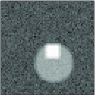
(a) Original image	(b) Disk component	(c) Square component

Figure 1: SPIN recovery of a noisy $64\times 64$ image from compressive measurements. The clean image consists of the linear superposition of a disk and a square of fixed pre-specified sizes, but the locations of the centers of the disk and the square are unknown. Additive Gaussian noise (SNR = 14dB) is added to the image prior to measurement. Signal length $N=64\times 64=4096$, number of compressive measurements $M=50.$ (a) Original noisy image. (b) Reconstructed disk. (c) Reconstructed square. SPIN perfectly reconstructs both components from just M/N = 1.2% measurements.

We generalize this setting to the case where the unknown signal of interest arises as a mixture of signals from two manifolds $\mathcal{A}$ and $\mathcal{B}$. For instance, suppose we are interested in the space of images, where $\mathcal{A}$ and $\mathcal{B}$ comprise of translations of fixed template images $f({\bf t})$ and $g({\bf t})$, where ${\bf t}$ denotes the 2D domain over which the image is defined. Then, the signal of interest is an image of the form

$${\bf x}^{*}={\bf a}^{*}+{\mathbf{b}}^{*}=f({\bf t}+\theta_{1})+g({\bf t}+\theta_{2}),$$

where $\theta_{1}$ and $\theta_{2}$ denote the unknown translation parameters. The problem is to recover $({\bf a}^{*},{\mathbf{b}}^{*})$, or equivalently $(\theta_{1},\theta_{2})$, given compressive measurements ${\bf z}=\mathbf{\Phi}({\bf a}^{*}+{\mathbf{b}}^{*})$.

We demonstrate that SPIN offers an easy, efficient technique to recover the component images. This example also demonstrates that SPIN is robust to practical considerations such as noise. Figure 1 displays the results of SPIN recovery of a $64\times 64$ image from very limited measurements. The unknown image consists of the linear sum of arbitrary translations of template images $f({\bf t})$ and $g({\bf t})$, that are smoothed binary images on a black background of a white disk and a white square, respectively. Further, the image has been contaminated with significant Gaussian noise (SNR = 14dB) prior to measurement (Fig. 1(a)). From Figs. 1(b) and 1(c), we observe that SPIN is able to perfectly recover the original component signals from merely $M=50$ random linear measurements.

For guaranteed SPIN convergence, we require that the manifolds $\mathcal{A},\mathcal{B}$ are incoherent. Informally, the condition of incoherence on the secants of $\mathcal{A}$ and $B$ is always valid when the template images $f({\bf t}),g({\bf t})$ are “sufficiently” distinct. This intuition is made precise using the bound in (3). More generally, we can state the following theoretical guarantee for SPIN performance in the case of general higher-dimensional manifolds.

Corollary 2 (SPIN for pairs of manifolds)

Let the entries of $\mathbf{\Phi}\in\mathbb{R}^{M\times N}$ be chosen from a standard Gaussian probability distribution. Let $\mathcal{A}$ and $\mathcal{B}$ be $\epsilon$-incoherent compact submanifolds of $\mathbb{R}^{N}$ of dimensions $K$ and $K^{\prime}$ respectively. Let ${\bf z}=\mathbf{\Phi}({\bf a}^{*}+{\mathbf{b}}^{*})$, where ${\bf a}^{*}\in\mathcal{A}$ and ${\mathbf{b}}^{*}\in\mathcal{B}$. Then, with high probability, SPIN exactly recovers $({\bf a}^{*},{\mathbf{b}}^{*})$ from ${\bf z}$, provided

$$M=\mathcal{O}\left(\left(K\log(C_{\mathcal{A}}N)+K^{\prime}\log(C_{\mathcal{B}}N)\right)\right).$$ (21)

Here, $C_{\mathcal{A}},C_{\mathcal{B}}$ are constants that depend only on certain intrinsic geometric parameters (such as the volume) of $\mathcal{A},\mathcal{B}$ respectively.

Proof. It is easy to see that if the matrix $\mathbf{\Phi}$ satisfies the RIP on the secants of the direct sum $\mathcal{C}=\mathcal{A}\oplus\mathcal{B}$, then SPIN recovery follows from Theorem 2. We show that a randomized construction of $\mathbf{\Phi}$ with number of rows specified by (21) satisfies the RIP on $\mathcal{C}$ with high probability. Essentially, our proof combines the techniques used in Section 3.2 of [18] with Lemma 1 of [25].

The manifold-embedding result in [18] is proved using two fundamental steps: (i) careful construction of a finite subset $\mathcal{R}$ of points in $\mathbb{R}^{N}$ that serves as a dense covering of the $K$-dimensional manifold of interest $\mathcal{A}$; and (ii) application of the Johnson-Lindenstrauss lemma [26] to this finite set $\mathcal{R}$ to produce, with vanishingly low probability of failure, a Gaussian measurement matrix $\mathbf{\Phi}$ that satisfies the RIP on $\mathcal{A}$. Section 3.2.5 of [18] indicates that the cardinality of the the finite set $\mathcal{R}$ can be upper bounded as

$$\#\mathcal{R}\leq(C_{\mathcal{A}}N)^{K},$$

where $C_{\mathcal{A}}$ is a constant that depends only on the intrinsic geometry of $\mathcal{A}$. However, in our setting we are interested in the direct sum of manifolds; correspondingly, we can construct finite sets $\mathcal{R}_{\mathcal{A}}$ and $\mathcal{R}_{\mathcal{B}}$ and apply Lemma 1 of [25], that specifies a lower bound on the number of measurements required to preserve the norms of linear sums of finite point sets:

$$M\geq\mathcal{O}\left(\log(\mathcal{R}_{\mathcal{A}}\mathcal{R}_{\mathcal{B}})\right)=\mathcal{O}\left(\left(K\log(C_{\mathcal{A}}N)+K^{\prime}\log(C_{\mathcal{B}}N)\right)\right),$$

where $K,K^{\prime}$ are the dimensions of $\mathcal{A},\mathcal{B}$ respectively. Corollary 2 follows.        $\Box$

An important consideration in SPIN is the tractable computation of the projection $\mathcal{P}_{\mathcal{M}}({\bf x})$ given any ${\bf x}\in\mathbb{R}^{N}$. For example, in the numerical example in Fig. 1, the operator $\mathcal{P}_{\mathcal{A}}({\bf x})$ onto the manifold $\mathcal{A}$ consists of running a matched filter between the template $f({\bf t})$ and the input signal ${\bf x}$ and returning $f({\bf t}+\widehat{\theta})$, where the parameter value $\widehat{\theta}$ corresponds to the 2D location of the maximum of the matched filter response. This is very efficiently carried out in $\mathcal{O}\left(N\log N\right)$ operations using the Fast Fourier Transform (FFT). However, for more complex articulation manifolds, the exact projection operation might not be tractable, whereas only approximate numerical projections can be efficiently computed. In this case also, SPIN can recover the signal components $({\bf a}^{*},{\mathbf{b}}^{*})$, but with weaker convergence guarantees (Theorem 3).

5.3 Signals in impulsive noise

In some situations, the signal of interest ${\bf x}$ might be corrupted with impulsive noise (or shot noise) prior to signal acquisition via linear measurements. For example, consider Fig. 2(a), where the Gaussian pulse is the signal of interest, and the spikes indicate the undesirable noise. In this case, the linear observations are more accurately modeled as:

$${\bf z}=\mathbf{\Phi}({\bf x}+{\bf n}),~{}~{}\textrm{such that}~{}{\bf x}\in\mathcal{M},$$

and ${\bf n}$ is a $K^{\prime}$-sparse signal in the canonical basis. Therefore, SPIN can be used to recover ${\bf x}$ from ${\bf z}$, provided that the manifold $\mathcal{M}$ is incoherent with the set of sparse signals $\Sigma_{K^{\prime}}$ and $\mathbf{\Phi}$ satisfies the RIP on the direct sum $\mathcal{M}+\Sigma_{K^{\prime}}$.

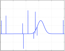
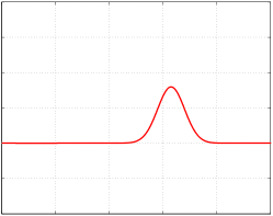
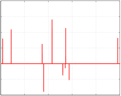
(a) Original signal	(b) Manifold component	(c) Noise component

Figure 2: SPIN recovery of a shifted Gaussian pulse from compressive measurements. The shift parameter of the pulse is unknown, and the signal is corrupted with $K^{\prime}$-sparse, impulsive noise of unknown amplitudes and locations. $N=10000,K^{\prime}=10,M=150.$ (a) Original signal. (b) Reconstructed Gaussian pulse (Recovery SNR = 80.09 dB). (c) Estimated noise component. SPIN perfectly reconstructs both components from just M/N = 1.5% measurements.

Figure 2 displays the results of a numerical experiment that illustrates the utility of SPIN in this setting. We consider a manifold of signals of length $N=10000$ that consist of shifts of a Gaussian pulse of fixed width ${\mathbf{g}}_{0}\in\mathbb{R}^{N}$. The unknown signal ${\bf x}$ is an element of this manifold $\mathcal{M}$, and is corrupted by $K^{\prime}=10$ spikes of unknown magnitudes and locations. This degraded signal is sampled using $M=150$ random linear measurements to obtain an observation vector ${\bf z}$.

We apply SPIN to recover ${\bf x}$ from ${\bf z}$. The projection operator $\mathcal{P}_{\mathcal{M}}(\cdot)$ consists of a matched filter with the template pulse ${\mathbf{g}}_{0}$, while the projection operator $\mathcal{P}_{\Sigma_{K^{\prime}}}(\cdot)$ simply returns the best $K^{\prime}$-term approximation in the canonical basis. Assuming that we have knowledge of the number of nonzeros in the noise vector ${\bf n}$, we can use SPIN to reconstruct both ${\bf x}$ and ${\bf n}$. We observe from Fig. 2(b) that SPIN recovers the true signal ${\bf x}$ with near-perfect accuracy. Further, this recovery is possible with only a small number $M=150$ linear measurements of ${\bf x}$, which constitutes but a fraction of the ambient dimension of the signal space.

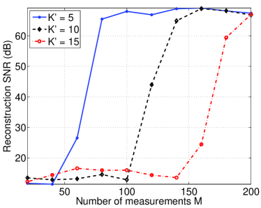
Figure 3: Monte Carlo simulation of SPIN signal recovery in impulsive noise , averaged over 100 trials. In each trial, the measured signal is the sum of a randomly shifted Gaussian pulse and a random $K^{\prime}$-sparse signal. SPIN can tolerate a higher number $K^{\prime}$ nuisance impulses by increasing the number of measurements $M$. By Corollary 2 this dependence of $M$ on $K^{\prime}$ can be shown to be linear.

Figure 3 plots the number of measurements $M$ vs. the signal reconstruction error (normalized relative to the signal energy and plotted in dB). We observe that, by increasing $M$, SPIN can tolerate an increased number $K^{\prime}$ of nuisance spikes. Further, by Corollary 2, we observe that this relationship between $M$ and $K^{\prime}$ is in fact linear. This result can be extended to any situation where the signals of interest obey a “hybrid” model that is a mixture of a nonlinear manifold and the set of sparse signals.

6 Discussion

We have proposed and rigorously analyzed an algorithm, which we dub Successive Projections onto INcoherent Manifolds (SPIN), for the recovery of a pair of signals given a small number of measurements of their linear sum. For SPIN to guarantee signal recovery, we require two main geometric criteria to hold: (i) the component signals should arise from two disjoint manifolds that are in a specific sense incoherent, and (ii) the linear measurement operator should satisfy a restricted isometry criterion on the secants of the direct sum of the two manifolds. The computational efficiency of SPIN is determined by the tractability of the projection operators onto either component manifold. We have presented indicative numerical experiments demonstrating the utility of SPIN, but defer a thorough experimental study of SPIN to future work.

Practical considerations. SPIN is an iterative gradient projection algorithm and requires as input parameters the number of iterations $T$ and the gradient step size $\eta$. The iteration count $T$ can be chosen using one of many commonly-used stopping criteria. For example, convergence can be declared if the norm of the error $\psi({\bf a}_{k},{\mathbf{b}}_{k})$ at the $(k+1)$-th time step does not differ significantly from the error at $k$-th time step. The choice of optimal step size $\eta$ is more delicate. Theorem 2 relates the step size to the restricted isometry constant $\delta$ of $\mathbf{\Phi}$, but this constant is not easy to calculate. In our preliminary findings, a step size in the range $0.5\leq\eta\leq 0.7$ consistently gave good results. See [27] for a discussion on the choice of step size for hard thresholding methods.

In practical scenarios, the signal of interest rarely belongs exactly to a low-dimensional submanifold $\mathcal{M}$ of the ambient space, but is only well-approximated by $\mathcal{M}$. Interestingly, in such situations the effect of this mismatch can be studied using the concept of $\gamma$-approximate projections (7). Theorem 3 rigorously demonstrates that SPIN is robust to such approximations. Further, our main result (Theorem 2) indicates that SPIN is stable with respect to inaccurate measurements, owing to the fact that the reconstruction error is bounded by a constant times the norm of the measurement noise vector ${\bf e}$.

More than two manifolds. For clarity and brevity, we have focused our attention on signals belonging to the direct sum of two signal manifolds. However, SPIN (and its accompanying proof mechanism) can be conceptually extended to sums of any $Q$ manifolds. In such a scenario, the conditions of convergence of SPIN would require that the component manifolds are $Q$-wise incoherent, and the measurement operator $\mathbf{\Phi}$ satisfies a restricted isometry on the $Q$-wise direct sum of the component manifolds.

Connections to matrix recovery. An intriguing open question is whether SPIN (or a similar first-order projected gradient algorithm) is applicable to situations where either of the component manifolds is the set of low-rank matrices. The problem of reconstructing, from affine measurements, matrices that are a sum of low-rank and sparse matrices has attracted significant attention in the recent literature [7, 28, 8]. The key stumbling block is that the manifold of low-rank matrices is not incoherent with the manifold of sparse matrices; indeed, the two manifolds share a nontrivial intersection (i.e., there exist low rank matrices that are also sparse, and vice versa). Phenomena such as these make the analysis of SPIN (or similar algorithms) quite challenging, and it may be that higher-order techniques will be needed for signal recovery.

References

- [1] S. Chen, D. Donoho, and M. Saunders, “Atomic decomposition by basis pursuit,” SIAM J. Sci. Comp., vol. 20, no. 1, pp. 33–61, 1998.
- [2] M. Elad, J.-L. Starck, P. Querre, and D. Donoho, “Simultaneous cartoon and texture image inpainting using morphological component analysis,” Appl. Comput. Harmon. Anal., vol. 19, no. 3, pp. 340–358, 2005.
- [3] J. Tropp, “Greed is good: Algorithmic results for sparse approximation,” IEEE Trans. Inform. Theory, vol. 50, no. 10, pp. 2231–2242, 2004.
- [4] E. Candès, “Compressive sampling,” in Proc. Int. Congress of Math., Madrid, Spain, Aug. 2006.
- [5] D. Donoho, “Compressed sensing,” IEEE Trans. Inform. Theory, vol. 52, no. 4, pp. 1289–1306, 2006.
- [6] M. Fazel, E. Candès, B. Recht, and P. Parrilo, “Compressed sensing and robust recovery of low rank matrices,” in Proc. 40th Asilomar Conf. Signals, Systems and Computers, Pacific Grove, CA, Nov. 2008.
- [7] E. Candès, X. Li, Y. Ma, and J. Wright, “Robust principal component analysis?,” J. ACM, vol. 58, no. 3, pp. 1–37, May 2011.
- [8] V. Chandrasekaran, S. Sanghavi, P. Parrilo, and A. Willsky, “Sparse and low-rank matrix decompositions,” in Proc. Allerton Conf. on Comm., Contr., and Comp., Monticello, IL, Sep. 2009.
- [9] I. Daubechies, M. Defrise, and C. De Mol, “An iterative thresholding algorithm for linear inverse problems with a sparsity constraint.,” Comm. Pure Appl. Math., vol. 57, no. 11, pp. 1413–1457, 2004.
- [10] T. Blumensath and M. Davies, “Iterative hard thresholding for compressive sensing,” Appl. Comput. Harmon. Anal., vol. 27, no. 3, pp. 265–274, 2009.
- [11] R. Meka, P. Jain, and I. Dhillon, “Guaranteed rank minimization via singular value projection,” in Proc. Adv. in Neural Processing Systems (NIPS), Vancouver, BC, Dec. 2010.
- [12] R. Garg and R. Khandekar, “Gradient descent with sparsification: an iterative algorithm for sparse recovery with restricted isometry property,” in Proc. Int. Conf. Machine Learning, Montreal, Canada, Jun. 2009.
- [13] P. Shah and V. Chandrasekharan, “Iterative projections for signal identification on manifolds,” in Proc. Allerton Conf. on Comm., Contr., and Comp., Monticello, IL, Sept. 2011.
- [14] D. Donoho, A. Maleki, and A. Montanari, “Message passing algorithms for compressed sensing,” Proc. Natl. Acad. Sci., vol. 106, no. 45, pp. 18914–18919, 2009.
- [15] Z. Lin, M. Chen, L. Wu, and Y. Ma, “The augmented Lagrange multiplier method for exact recovery of corrupted low-rank matrices,” Arxiv preprint arXiv:1009.5055, 2010.
- [16] M. McCoy and J. Tropp, “Sharp recovery bounds for convex deconvolution, with applications,” Arxiv preprint arXiv:1205.1580, 2012.
- [17] M. Wakin, The Geometry of Low-Dimensional Signal Models, Ph.D. thesis, Rice University, Aug. 2006.
- [18] R. Baraniuk and M. Wakin, “Random projections of smooth manifolds,” Found. Comput. Math., vol. 9, no. 1, pp. 51–77, 2009.
- [19] M. Elad and A. Bruckstein, “A generalized uncertainty principle and sparse representation in pairs of bases,” IEEE Trans. Inform. Theory, vol. 48, no. 9, pp. 2558–2567, 2002.
- [20] C. Studer, P. Kuppinger, G. Pope, and H. Bölcskei, “Recovery of sparsely corrupted signals,” IEEE Trans. Inform. Theory, 2012, To appear.
- [21] A. Feuer and A. Nemirovski, “On sparse representation in pairs of bases,” IEEE Trans. Inform. Theory, vol. 49, no. 6, pp. 1579–1581, 2003.
- [22] R. Gribonval and M. Nielsen, “Sparse representations in unions of bases,” IEEE Trans. Inform. Theory, vol. 49, no. 12, pp. 3320–3325, 2003.
- [23] C. Grimes and D. Donoho, “Image manifolds which are isometric to euclidean space,” J. Math. Imag. and Vision, vol. 23, no. 1, pp. 5–24, 2005.
- [24] M. Wakin, D. Donoho, H. Choi, and R. Baraniuk, “High-resolution navigation on non-differentiable image manifolds,” in Proc. IEEE Int. Conf. Acoust., Speech, and Signal Processing (ICASSP), Philadelphia, PA, Mar. 2005.
- [25] M. Davenport, P. Boufounos, M. Wakin, and R. Baraniuk, “Signal processing with compressive measurements,” IEEE J. Select. Top. Signal Processing, vol. 4, no. 2, pp. 445–460, 2010.
- [26] W. Johnson and J. Lindenstrauss, “Extensions of Lipschitz mappings into a Hilbert space,” in Proc. Conf. Modern Anal. and Prob., New Haven, CT, Jun. 1982.
- [27] A. Kyrillidis and V. Cevher, “Recipes for hard thresholding methods,” Tech. Rep., EPFL, Oct. 2011.
- [28] A. Waters, A. Sankaranarayanan, and R. Baraniuk, “SpaRCS: Recovering low-rank and sparse matrices from compressive measurements,” in Proc. Adv. in Neural Processing Systems (NIPS), Granada, Spain, Dec. 2011.