How Flow Changes Polymer Depletion in a Slit

Abstract

A theoretical model is developed for predicting dynamic polymer depletion under the influence of fluid flow. The results are established by combining the two-fluid model and the self-consistent field theory. We consider a uniform fluid flow across a slit containing a solution with polymer chains. The two parallel and infinitely long walls are permeable to solvent only and the polymers do not adsorb to these walls. For a weak flow and a narrow slit, an analytic expression is derived to describe the steady state polymer concentration profiles in a $\Theta$-solvent. In both $\Theta$- and good-solvents, we compute the time evolution of the concentration profiles for various flow rates characterized by the Peclet number. The model reveals the interplay of depletion, solvent condition, slit width, and the relative strength of the fluid flow.

1 Introduction

In a polymer solution near an interface the polymer segments are either attracted or repelled by that interface Fleer1993 . In the latter case there exists a depletion zone near the interface. In this zone the polymer segment concentration is smaller than the bulk value because of the less possible number of configurations of the polymer chains. The non-adsorbing wall forbids a certain amount of paths of the polymer chain. For ideal polymer chains near a hard wall the depletion thickness is close to the polymer’s radius of gyration Eisenriegler1983 . This result holds generally for a dilute polymer solution Hanke1999 ; Fleer2008 , whereas in a semi-dilute polymer solution the depletion thickness is determined by the correlation length deGennes_scaling_concept1979 . These results for dilute and semi-dilute concentrations can also be combined Fleer2003 ; Fleer2007 . The previous investigations of polymer depletion at an interface primarily focus on the equilibrium case. The equilibrium depletion thickness suffices to describe the attraction between colloidal particles when the depletion layers overlap Asakura1954 ; Vrij1976 , which can be measured for instance by optical tweezers Verma2000 . The depletion force may yield phase transitions Lekkerkerker1992 ; Ilett1995 ; Meijer1994 for which the binodals can be predicted for well-defined colloid-polymer mixtures Fleer2008 ; Tuinier2008 . It is of fundamental and practical interest to understand the change of the depletion layer under a fluid flow effect. Simple shear flow of a polymer solution next to a single wall leads to a slip-like behavior even if the depletion layer is assumed to be unaffected by shear Tuinier2005 . It has been shown, however, that the flow does change the depletion thickness at a wall Duering1990 . In colloidal systems, the models developed for single particle motion and pairwise particle interactions neglect the slight distortion of the depletion zone Tuinier2006 ; Fan2007 ; Fan2010 . This is applicable for describing long-time Brownian diffusion with weak convective effect. A convective depletion model was first established by Odijk for describing a thin depletion boundary layer in front of a fast moving sphere Odijk2004 . However, a complete picture of the fully coupled convective depletion effect under various solution conditions is not yet available.

In this paper we propose a theoretical framework to investigate dynamic depletion effects by combining two models : (i) the two-fluid model Doi1992 , with the chemical potential obtained under the ground state approximation (GSA) of the self-consistent field theory (SCFT) for polymeric systems Fleer1993 ; deGennes_scaling_concept1979 and (ii) the two-fluid model along with the dynamical version (DSCFT) Hall2007 of SCFT. To demonstrate how the combined formalism works well, here we study the influence of flow on the polymer segment density profile in a narrow or wide slit. This is an interesting problem since for a narrow slit an analytic expression is only available for describing the equilibrium segment density profile Fleer1993 ; Fleer2003 . It is unclear that to what extent a flow field modifies the depletion layers. Flow through pores is relevant for instance in size-exclusion chromatography, which is widely used to analyze polymersPore .

The content of this paper is as follows. In the next section, we start from a general formulation of the two-fluid model for polymer transport to resolve the interplay of convective and diffusive effects. Then, in Sec. 2.2 we describe the ground state approximation of SCFT and the dynamical version of SCFT to express the chemical potential which characterizes the segment density profiles under various flow conditions. In Sec. 2.3, we describe a set of equations to investigate the dynamics of polymer segment depletion in a slit. In Sec. 3, the results for both $\Theta$- and good-solvent conditions are provided in detail. Finally, we give a conclusion in Sec. 4.

2 Theory

Here we describe theoretical models to investigate dynamic depletion effects under a flow. The models used here are combinations of the two fluid model with a model to evaluate the chemical potential for polymeric systems, i.e., (i) the two-fluid models with a chemical potential evaluated under GSA of SCFT and (ii) two fluid model with DSCFT. The validity for each model has been reported in literature. The two-fluid model of polymeric materials was developed by Doi and Onuki Doi1992 . The model has succeeded in explaining the viscoelastic behaviors R1 ; R2 and shear induced phase separation in polymer solutions and polymer blends R3 . The validity of the model has been confirmed by simulations R2 ; R3 and experiments R1 ; R4 , and thus is suitable to describe non-equilibrium transport phenomena in polymeric systems. The SCFT is frequently used for predicting the equilibrium properties of inhomogeneous polymeric systems. It gives a precise evaluation of chemical potential for each constituent in the system Fleer1993 ; deGennes_scaling_concept1979 . In the two-fluid model, the determination of the local chemical potential of polymer segment is critical especially for the reduction of the possible chain conformations near the wall (the depletion effect). Therefore, SCFT theory is more suitable than Flory-Huggins theory which was developed for evaluating bulk properties. The computational costs of SCFT are higher than using the Flory-Huggins theory because the statistical weight of each polymer conformation must be evaluated by solving a diffusion-like differential equation unless the ground state approximation is used, which is applicable when the gyration radius of the constituent polymers is sufficiently large compared to the length scale of the confined space. At equilibrium, the GSA for the depletion layer near a flat wall agrees well with the numerical and Monte Carlo simulation results RemcoBook2011 ; R5 . When the system is out of equilibrium under a constant flow condition, a dynamical version of SCFT (DSCFT) is needed to study the polymer depletion effect. The validity and efficiency of DSCFT for various cases has been reported in the literature Hall2007 .

In the following subsections, we briefly explain the essence of the two-fluid model, dynamical version of the self-consistent field theory and the ground state approximation applied to the SCFT.

2.1 Two-Fluid Model

We consider inertialess fluid motion and polymers in dilute to semi-dilute polymer solutions. The polymer solution consists of solvent and homopolymer with length $aN$, where $a$ and $N$ are the monomer size and the polymerization index, respectively. The transient-evolution of polymer segment volume fraction $\phi_{\rm{p}}$ is given by the continuity equation :

$${\partial\phi_{\rm{p}}(\vec{r},t)\over\partial t}=-\nabla\cdot(\phi_{\rm{p}}\vec{v}_{\rm{p}}),$$ (1)

where $t$ is time, $\vec{v}_{\rm{p}}$ is the velocity of the polymer segments in the fluid, $\phi_{\rm{p}}(\vec{r},t)=a^{3}{\rho}_{\rm{p}}(\vec{r},t)$ with $a$ being the segment length and $\rho_{\rm{p}}$ the local number density of polymer segments. The local volume fraction of solvent is $\phi_{\rm{s}}$. Because $\phi_{\rm{p}}+\phi_{\rm{s}}=1$, the total velocity $\vec{v}(\vec{r},t)=\phi_{\rm{p}}\vec{v}_{\rm{p}}+\phi_{\rm{s}}\vec{v}_{\rm{s}}$ ($\vec{v}_{\rm{s}}$ is the solvent velocity) satisfies the incompressibility condition $\nabla\cdot\vec{v}=0$. The momentum equation of the two-fluid model can be derived from the Rayleighian given by Doi and Onuki Doi1992 :

$${\cal R}=\int\biggr{[} {{\zeta}(\vec{r},t)\over 2}|\vec{v}_{\rm{p}}-\vec{v}_{\rm{s}}|^{2}-\mu_{\rm{p}}\nabla\cdot(\phi_{\rm{p}}\vec{v}_{\rm{p}})-\mu_{\rm{s}}\nabla\cdot(\phi_{\rm{s}}\vec{v}_{\rm{s}})$$ (2)

$$-p\nabla\cdot\vec{v}+\vec{\sigma}_{\rm{p}}:\nabla\vec{v}_{\rm{p}}+\vec{\sigma}_{\rm{s}}:\nabla\vec{v}_{\rm{s}}\biggr{]}d\vec{r},$$

where $\mu_{\rm{p}}$, $\mu_{\rm{s}}$, $\vec{\sigma}_{\rm{p}}$, $\vec{\sigma}_{\rm{s}}$, and $p$ are the local chemical potential of polymer and solvent, the deviatoric stress of polymer and solvent, and the hydrodynamic pressure, respectively. The friction coefficient ${\zeta}$ between the two fluids can be approximated as Stokes friction coefficient for the polymer blob per volume deGennes_scaling_concept1979 , $\zeta=6\pi\eta_{\rm{s}}\xi/\xi^{3}=6\pi\eta_{\rm{s}}/\xi^{2}$, where $\xi(\phi_{\rm{p}})$ is the blob size and $\eta_{\rm{s}}$ is the solvent viscosity. The blob size is related to $\phi_{\rm{p}}$ as $\xi\simeq a\phi_{\rm{p}}^{-m}$ deGennes_scaling_concept1979 , where $m=1$ and $3/4$ for $\Theta$- and good solvents, respectively. By minimizing $\cal R$ with respect to $\vec{v}_{\rm{p}}$ and $\vec{v}_{\rm{s}}$, the following momentum equations can be derived :

$${\zeta}(\vec{v}_{\rm{p}}-\vec{v}_{\rm{s}})+\phi_{\rm{p}}\nabla p+\phi_{\rm{p}}\nabla\mu_{\rm{p}}-\nabla\cdot\vec{\sigma}_{\rm{p}}=0,$$ (3)

$${\zeta}(\vec{v}_{\rm{s}}-\vec{v}_{\rm{p}})+\phi_{\rm{s}}\nabla p+\phi_{\rm{s}}\nabla\mu_{\rm{s}}-\nabla\cdot\vec{\sigma}_{\rm{s}}=0.$$ (4)

By combining Eqs.(3) and (4) we obtain

$$\nabla\cdot\vec{\sigma}-\nabla P-\nabla\cdot\vec{\pi}=0,$$ (5)

where the total stress $\vec{\sigma}=\vec{\sigma}_{\rm{p}}+\vec{\sigma}_{\rm{s}}$, $P$ is the modified pressure defined by $P=p+\mu_{\rm{s}}$, and $\vec{\pi}$ is the osmotic pressure tensor defined as

$$\nabla\cdot\vec{\pi}=\phi_{\rm{p}}(\vec{r},t)\nabla\mu(\vec{r},t),$$ (6)

where $\mu=\mu_{\rm{p}}-\mu_{\rm{s}}$ is the difference between the chemical potentials. Substituting Eq.(5) into Eq.(4) and eliminating $P$, the following expression for the polymer velocity is obtained:

$$\vec{v}_{\rm{p}}\simeq \vec{v}-{\phi_{\rm{s}}\over{\zeta}}\biggr{[}\phi_{\rm{s}}\bigr{(}\nabla\cdot\vec{\pi}-\nabla\cdot\vec{\sigma}_{\rm{p}}\bigr{)}+\phi_{\rm{p}}\nabla\cdot\vec{\sigma}_{\rm{s}}\biggr{]}.$$ (7)

In this paper we consider $\phi_{\rm{p}}\ll 1$ for dilute and semi-dilute solutions, and $\phi_{\rm{p}}\nabla\cdot\vec{\sigma}_{\rm{s}}$ of the above equation is negligible. The polymer velocity relative to the total velocity is driven by the osmotic pressure and the deviatoric stress of the polymer fluid. Substituting Eq.(7) into Eq.(1) yields the polymer transport equation :

$${\partial\phi_{\rm{p}}\over\partial t}+\nabla\cdot(\phi_{\rm{p}}\vec{v})\simeq\nabla\cdot\biggr{[}{\phi_{\rm{p}}\phi_{\rm{s}}^{2}\over{\zeta}(\phi_{\rm{p}})}\biggr{(}\phi_{\rm{p}}\nabla\mu-\nabla\cdot\vec{\sigma}_{\rm{p}}\biggr{)}\biggr{]}.$$ (8)

This formulation is consistent with Odijk’s work Odijk2004 except for the $\phi_{\rm{p}}$-dependent friction coefficient and the additional $\nabla\cdot\vec{\sigma}_{\rm{p}}$ term. For a solid object with an arbitrary shape $\Omega$ with a surface $\partial\Omega$, the osmosis-induced force and torque are $\vec{f}=\int_{\partial\Omega}(-\vec{\pi}\cdot\vec{n})dS$ and $\vec{T}=\int_{\partial\Omega}\vec{R}\times(-\vec{\pi}\cdot\vec{n})dS$, respectively, where $\vec{n}$ is the surface normal and $\vec{R}$ is the vector from the center of gravity to the surface of the object.

When assume that the polymer stress in the dilute and semi-dilute ($\bar{\phi}_{\rm{p}}\hskip 3.00003pt\raisebox{1.72218pt}{$<$}\raisebox{-3.01385pt}{$\sim$}\hskip 3.00003pt$ overlap volume fraction $\phi_{\rm{p}}^{\ast}\simeq N^{1-3\nu}$) polymer solution can be expressed as $\eta^{\prime}\phi_{\rm{p}}\bigr{(}\nabla\vec{v}+{}(\nabla\vec{v})^{\rm{T}}\bigr{)}$, where $\eta^{\prime}$ is a constant. Hence the total velocity follows as $\vec{v}\sim{\cal O}({\bar{\phi}}_{\rm{p}}^{2})$, as seen from Eq.(5) and $\vec{\pi}\sim{\cal O}(\bar{\phi}_{\rm{p}}^{2})$, and thus $\nabla\cdot\vec{\sigma}_{\rm{p}}\sim{\cal O}(\bar{\phi}_{\rm{p}}^{3})$. Also because $\mu\sim{\cal O}({\bar{\phi}}_{\rm{p}})$, so $\phi_{\rm{p}}\nabla\mu_{\rm{p}}\sim{\cal O}(\bar{\phi}_{\rm{p}}^{2})$, this implies ${\cal O}(\nabla\cdot\vec{\sigma}_{\rm{p}})\ll{\cal O}(\phi_{\rm{p}}\nabla\mu)$ and the polymer force $\nabla\cdot\vec{\sigma}_{\rm{p}}$ in Eq.(8) is indeed negligible Odijk2004 .

2.2 Chemical Potential of Polymers

2.2.1 Self-Consistent Field Theory

Using SCFT, the Helmholtz free energy is written as

$${F\over k_{\rm{B}}T}={1\over a^{3}}\int \biggr{[}\chi\phi_{\rm{p}}\phi_{\rm{s}}-w_{\rm{p}}\phi_{\rm{p}}-w_{\rm{s}}\phi_{\rm{s}}\biggr{]}d\vec{r}$$ (9)

$$-{\bar{\phi}_{\rm{p}}\over N}\ln({NQ_{\rm{p}}\over{V\bar{\phi}_{\rm{p}}}})-{\bar{\phi}_{\rm{s}}}\ln({Q_{\rm{s}}\over{V\bar{\phi}_{\rm{s}}}}),$$

where $N$ is the number of segment in a single chain, $V$ is the volume of the system, and $w_{\alpha}$ and $\bar{\phi}_{\alpha}$ are the local dimensionless interaction field (scaled by $k_{\rm{B}}T$) and the average volume fraction of polymer segments in the bulk for the $\alpha$-component ($\alpha$ represents polymer or solvent), respectively. The partition functions $Q_{\rm{p}}$ and $Q_{\rm{s}}$ for a single chain and a single solvent, respectively, are defined by

$$Q_{\rm{p}}= \int_{V}d\vec{r}\int_{0}^{1}q(\vec{r},s)q(\vec{r},1-s)ds,$$ (10)

and

$$Q_{\rm{s}}= \int_{V}d\vec{r}\exp(-w_{\rm{s}}(\vec{r})).$$ (11)

In Eq.(10), $q$ is the statistical weight of the polymer chain and can be calculated by

$${\partial q\over\partial s}={a^{2}\over 6}N\nabla^{2}q-Nw_{\rm{p}}(\vec{r})q\quad{\rm for}\quad 0\leq s\leq 1$$ (12)

with the initial condition $q(\vec{r},0)=1$ and the zero boundary condition at the solid surface $q(\vec{r}\in\partial\Omega)=0$ for an arbitrary contour coordinate $s$.

In order to evaluate $\mu_{\rm{p}}$ and $\mu_{\rm{s}}$ for a given $\phi_{\rm{p}}(\vec{r},t)$, the following iterative procedure can be used Hall2007 :

i) Find $w_{\rm{p}}(\vec{r})$ and $q(\vec{r},s)$ that satisfy Eq.(12) and

$${1\over Q_{\rm{p}}}\int_{0}^{1}q(\vec{r},s)q(\vec{r},1-s)ds={1\over V\bar{\phi}_{\rm{p}}}\phi_{\rm{p}}(\vec{r},t)$$ (13)

along with the initial and boundary conditions.

ii) Evaluate $w_{\rm{s}}(\vec{r})$ that satisfies

$${1\over Q_{\rm{s}}}\exp(-w_{\rm{s}}(\vec{r}))={1\over V\bar{\phi}_{\rm{s}}}\phi_{\rm{s}}(\vec{r},t).$$ (14)

iii) Compute the chemical potential difference $\mu=\mu_{\rm{p}}-\mu_{\rm{s}}$ from the functional derivatives:

$$\mu_{\rm{p}}(\vec{r})= {\delta F\over\delta\phi_{\rm{p}}}=-w_{\rm{p}}(\vec{r})+\chi\phi_{\rm{s}}(\vec{r}),$$ (15)

$$\mu_{\rm{s}}(\vec{r})= {\delta F\over\delta\phi_{\rm{s}}}=-w_{\rm{s}}(\vec{r})+\chi\phi_{\rm{p}}(\vec{r}).$$ (16)

iv) Finally, the time evolution of $\phi_{\rm{p}}(\vec{r},t)$ can be calculated by Eq.(8) with $\vec{\sigma}_{\rm{p}}=\vec{0}$.

2.2.2 Ground State Approximation

In a confined space (Fig.1) we can apply the ground state approximation (GSA) to the self-consistent field theory (SCFT). The Helmholtz free energy of the mixture can be expressed as deGennes_scaling_concept1979

$$F=\epsilon_{\rm{o}}\int\biggr{[}\ell^{2}(\nabla\sqrt{\phi_{\rm{p}}})^{2}+f_{\rm{o}}(\phi_{\rm{p}})\biggr{]}d\vec{r},$$ (17)

where ${\epsilon_{\rm{o}}=k_{\rm{B}}T/a^{3}}$, $\ell^{2}={a^{2}/6}$ in GSA or $\ell^{2}={a^{2}/9}$ in the random phase approximation (RPA), $f_{\rm{o}}(\phi_{\rm{p}})=(1-\phi_{\rm{p}})\ln(1-\phi_{\rm{p}})+\chi\phi_{\rm{p}}(1-\phi_{\rm{p}}),$ and $\chi$ is the Flory-Huggins parameter. The reason why a translational entropy term $\phi_{\rm{p}}/N\ln\phi_{\rm{p}}$ does not appear in $f_{\rm{o}}$ has been explained by Fredrickson BookOfFredrickson . The chemical potential difference $\mu$ is determined by the functional derivative of $F$ with respect to $\phi_{\rm{p}}$:

$$\mu(\vec{r})=\epsilon_{\rm{o}}\biggr{[}-{\ell^{2}\over\sqrt{\phi_{\rm{p}}}}\nabla^{2}\sqrt{\phi_{\rm{p}}}+(1-2\chi)\phi_{\rm{p}}\biggr{]}.\qquad$$ (18)

Since $\phi_{\rm{p}}$ is much smaller than unity, only the zeroth- and first-order terms involving $\phi_{\rm{p}}$ in the chemical potential are preserved. The corresponding osmotic stress tensor $\pi_{ij}$, scaled by $\epsilon_{\rm{o}}$, can be expressed as

$$\pi_{ij}=\biggr{\{}\Bigr{[}\pi_{\rm{o}}-\ell^{2}\nabla\cdot\bigr{(}\sqrt{\phi_{\rm{p}}}\nabla\sqrt{\phi_{\rm{p}}}\bigr{)}\Bigr{]}\delta_{ij}$$

$$\qquad\qquad\qquad+2\ell^{2}{\partial\sqrt{\phi_{\rm{p}}}\over\partial x_{i}}{\partial\sqrt{\phi_{\rm{p}}}\over\partial x_{j}}\biggr{\}},$$ (19)

where $\pi_{\rm{o}}(\phi_{\rm{p}})=\phi_{\rm{p}}f^{\prime}_{\rm{o}}(\phi_{\rm{p}})-f_{\rm{o}}$ is the osmotic pressure in the bulk. Note that $\nabla\cdot\vec{\pi}$ satisfies Eq.(6).

2.3 One-dimensional Formulation

We focus on non-equilibrium polymer segment concentration profiles under a uniform flow $U$ passing through two parallel and solvent-permeable walls separated by a distance $L$ (Fig.1).

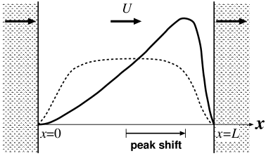
Figure 1: A schematic illustration of the convective depletion effect on the polymer segment profile (solid line) in a slit between two parallel and solvent permeable walls. The dashed line indicates the equilibrium distribution. The polymer concentration vanishes at the walls.

There are three length scales involved in this problem, i.e., the width $L$, the monomer size $a$, and gyration radius $R_{\rm{g}}$ of the ideal polymer chain, defined as $R_{\rm{g}}=a(N/6)^{1/2}$. We select $L$ as the length scale, and $\tau\equiv L^{2}/D$ as the time scale, where $D$ is a diffusion coefficient defined by $D={\bar{\phi}_{\rm{p}}}^{1-2m}D_{\rm self}$, where $D_{\rm self}={k_{\rm{B}}T/6\pi\eta_{\rm{s}}a}$ is the self-diffusion coefficient of a single polymer segment. It should be noted that the factor $\bar{\phi}_{\rm{p}}^{1-2m}$ comes from the fact that a polymer segment is not affected directly by hydrodynamic flow, but a blob with a size $\xi$ as a whole is affected by hydrodynamic flow, in a way that the friction constant was introduced as $\zeta(\phi_{\rm{p}})=6\pi\eta_{\rm{s}}\xi/$[blob volume]. The volume fraction of polymer is scaled by the averaged volume fraction $\bar{\phi}_{\rm{p}}$, and the chemical potential is scaled by $k_{\rm{B}}T/a^{3}$. Hereafter we use dimensionless expressions. The scaled chemical potential difference is expressed as

$$\mu=-{\ell^{2}\over L^{2}}{1\over\varphi}{\partial^{2}\varphi\over\partial x^{2}}+{v}\varphi^{2},$$ (20)

where $\ell=(a^{2}/6)^{1/2}$, $v=(1-2\chi)\bar{\phi}_{\rm{p}}$ and $\varphi=(\phi_{\rm{p}})^{1/2}$. Note that the ground-state approximation, Eq.(20) is valid only for a narrow slit $L/R_{\rm{g}}<\pi$ deGennes_scaling_concept1979 . The polymer transport equation (Eq.(8)) thus can be expressed as

$${\partial\varphi^{2}\over\partial t}+{\sf Pe}{\partial\varphi^{2}\over\partial x}={\partial\over\partial x}\biggr{[}\varphi^{2(2-2m)}{\partial\mu\over\partial x}\biggr{]},$$ (21)

where ${\sf Pe}=UL/D$ is the Peclet number and the width of the slit $L$ is the characteristic length of the system. The control parameters are ${\sf Pe}$, $v$, and $L/\ell$. The translational entropy term containing the polymerization index $N$ only appears in a wide slit case ($L\gg R_{\rm{g}}$), but not in the transport equation, eq.(21) with eq.(20), for the narrow slit case under GSA. Since the polymer solution we consider consists of homopolymer and solvent, the monomer size $a$ is not a parameter but a fixed constant. Hence, using $R_{\rm{g}}\equiv\ell N^{1/2}$, the intrinsic control parameters in the present system are found to be ${\sf Pe},v,$ and $L/R_{\rm{g}}.$ It should be noted that the average volume fraction $\bar{\phi}_{\rm{p}}$ is included implicitly in $v$ as $v=(1-2\chi)\bar{\phi}_{\rm{p}}$. In the following numerical calculations, we applied various values, the Flory parameter $\chi$ to realize variations in the excluded volume parameter $v$. The value of $\bar{\phi}_{\rm{p}}$ is selected to be close to or less than the overlap volume fraction $\phi_{\rm{p}}^{\ast}$ because the viscoelastic effect ($\vec{\sigma}_{\rm{p}}$ in eq.(8)) is neglected here. When the average volume fraction is much smaller than $\phi_{\rm{p}}^{\ast}$, the system gives almost the same behavior as $\Theta$-solvent due to the effectively small excluded volume effect ($v\simeq 0$). From the above reason, we consider $\bar{\phi}_{\rm{p}}\simeq\phi_{\rm{p}}^{\ast}$.

By applying a constant flow with uniform velocity $U$ at $t=0$ to a quiescent polymer solution in a slit, polymer segments start to accumulate at a region near the wall on the downstream side and then the system reaches a steady state with a region of accumulated polymer segments, characterized by a peak at which the polymer segment concentration passes through a maximum. The corresponding convective or accumulation time scale can be estimated by $t^{\ast}=L/U$. Hereinafter we refer to it as ”accumulation time”. So, the dimensionless accumulation time is ${\tilde{t}}^{\ast}(\equiv t^{\ast}/\tau)$ $\sim 1/{\sf Pe}$. Note that in the estimation of $t^{\ast}$ the distance of the peak shift is less than $L$ and the effective advection velocity is probably smaller than $U$ due to the thermodynamic flux which tends to reduce concentration gradients.

Because the walls are not permeable to polymers, the corresponding boundary conditions are $\varphi(0)$=0 and $\varphi(1)$=0, and the zero flux boundary conditions $d\mu/dx{|}_{x=0}$=0 and ${d\mu/dx}{|}_{x=1}$=0 are applied. Equation (21) leads to the steady state solution:

$$\mu(x)-\mu(0)={\sf Pe}~{}\int_{0}^{x}\varphi^{2(2m-1)}(x^{\prime})dx^{\prime}.$$ (22)

Under a weak flow condition, ${\sf Pe}\ll 1$, the first-order approximation of the steady state solution for $\varphi$ and $\mu$ can be written as

$$\varphi(x)=\sqrt{\phi_{\rm{p}}(x)}\simeq\varphi_{\rm{o}}(x)+{\sf Pe}~{}\varphi_{1}(x),$$ (23)

and

$$\mu(x)\simeq\mu_{\rm{o}}(x)+{\sf Pe}~{}\mu_{1}(x).$$ (24)

By substituting Eqs.(23) and (24) into Eq.(22), the corresponding leading and first-order equations become

$${\ell^{2}\over L^{2}}{d^{2}\varphi_{\rm{o}}\over dx^{2}}-v\varphi_{\rm{o}}^{3}+{\mu_{\rm{o}}(0)\varphi_{\rm{o}}}=0,$$ (25)

and

$$\biggr{[}~{}{\ell^{2}\over L^{2}}{d^{2}\over dx^{2}}+\mu_{\rm{o}}(0)-3v\varphi_{\rm{o}}^{2}~{}\biggr{]}\varphi_{1}=$$

$$\quad-\varphi_{\rm{o}}(x)\biggr{[}\mu_{1}(0)+\int_{0}^{x}\varphi_{\rm{o}}^{2(2m-1)}(x^{\prime})dx^{\prime}\biggr{]},\quad$$ (26)

respectively. Both $\varphi_{0}$ and $\varphi_{1}$ vanish at the walls. Next we consider the results for $\Theta$- and good-solvent cases under narrow and wide slit conditions.

3 Results and Discussion

3.1 $\Theta$-solvent Cases

3.1.1 Narrow Slit, $L<\pi R_{\rm{g}}$

The ground state approximation is valid when the distance between two walls is small, i.e., $L<\pi R_{\rm{g}}$. Equation (20) with $v=0$ and Eq.(21) are used to investigate the time evolution of polymer segment concentration profile. Under steady and weak flow conditions in $\Theta$-solvent ($m=1$, $\nu=0$), Eqs.(25) and (26) reduce to

$${\ell^{2}\over L^{2}}{d^{2}\varphi_{\rm{o}}\over dx^{2}}=-{\mu_{\rm{o}}(0)\varphi_{\rm{o}}},$$ (27)

and

$$\biggr{[}{\ell^{2}\over L^{2}}{d^{2}\over dx^{2}}+\mu_{\rm{o}}(0)\biggr{]}\varphi_{1}=$$

$$\qquad\quad-\varphi_{\rm{o}}(x)\biggr{[}\mu_{1}(0)+\int_{0}^{x}\varphi_{\rm{o}}^{2}(x^{\prime})dx^{\prime}\biggr{]}.\qquad$$ (28)

Figure 2: Steady state polymer segment volume fraction $\phi_{\rm{p}}(x,t=\infty)$ of a polymer solution ($\bar{\phi}_{\rm{p}}=0.1$, $N=1000$ and $\chi=0.5$) in a slit ($L/R_{\rm{g}}=1$, where $R_{\rm{g}}\simeq 33\ell$) at Pe=0, 0.5, 1.0, and 1.5 $\times 10^{-2}$. The solid lines are from the numerical solutions of Eqs.(20) and (21). The symbols ($+$, $\times$, $\ast$, $\sqcup\!\!\!\!\sqcap$) indicate the analytical approximations for Pe=0, 0.5, 1.0, and 1.5 $\times 10^{-2}$, respectively.

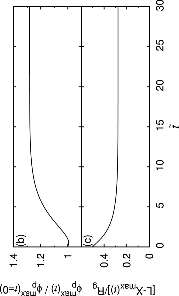
Figure 3: (a) Transient evolutions of the segment concentration profiles $\phi_{\rm{p}}(x,t)$, (b) the peak concentration and (c) the distance from the peak position to the downstream-side wall. Applied parameters are: $\bar{\phi}_{\rm{p}}=0.1$, $N=1000$, $\chi=0.5$, $L/R_{\rm{g}}=1$, and Pe=0.05 at $\tilde{t}=t/\tau\geq 0$. The profiles shown in (a) are at $\tilde{t}=$0 (no flow), 1, 2, 4, 8, 16 and 32. At ${\tilde{t}}{{>}\atop{\sim}}12$, the profile approaches a steady state as can be seen in panels (b) and (c).

The zeroth-order solution corresponding to the equilibrium state is deGennes_scaling_concept1979 :

$$\varphi_{\rm{o}}(x)=\sqrt{\phi_{\rm{o}}(x)}=\sqrt{2}\sin(\pi x)~{}~{}{\rm for}\quad 0\leq x\leq 1,$$ (29)

which satisfies the normalization condition, $\int_{0}^{1}\phi_{\rm{o}}(x)dx$$=1$, and thus $\mu_{\rm{o}}(0)=\pi^{2}\ell^{2}/L^{2}$. The first-order solution reads

$$\varphi_{1}(x) =A\sin(\pi x)$$ (30)

$$-B\bigr{\{}~{}(1+8\pi^{2}x-8\pi^{2}x^{2})\cos(\pi x)$$

$$\qquad~{}~{}-\cos(3\pi x)+4\pi x\sin(\pi x)~{}\bigr{\}},\qquad$$

where the constant $B=L^{2}/16\ell^{2}\pi^{3}\sqrt{2}$ and $\mu_{1}(0)$ in Eq.(28) is found to be $-1/2$ by the boundary condition $\varphi_{1}(1)=0$. The constant $A$ can be determined by the normalization condition $\int_{0}^{1}\phi(x)dx=1$, and we obtain

$$A =2\pi B+{B^{2}\over\sqrt{2}}\Bigr{(}77-2\pi^{2}-{16\over 15}\pi^{4}\Bigr{)}{\sf Pe}+{\cal O}({\sf Pe}^{2}).\quad$$ (31)

Accordingly, the peak value and its location can be expressed as

$${{\phi_{\rm{p}}^{\rm max}({\sf Pe})\over\phi_{\rm{p}}^{\rm max}(0)}} =1+B^{2}\Bigr{(}77-2\pi^{2}+{14\over 15}\pi^{4}\Bigr{)}{\sf Pe^{2}}+\cdots$$ (32)

and

$$x_{\rm max} ={1\over 2}\Bigr{[}1+2\sqrt{2}\pi B{\sf Pe}+{\cal O}({\sf Pe}^{3})\Bigr{]}.$$ (33)

From eq.(19), the osmotic stresses acting on the walls at $x=0$ and $x=1$ are

$$\pi_{xx}=\epsilon_{\rm{o}}\pi^{2}{\bar{\phi}_{\rm{p}}}{\ell^{2}\over L^{2}}\biggr{[}\sqrt{2}\mp\big{(}6\pi B{\sf Pe}+C{\sf Pe}^{2}\big{)}\biggr{]}^{2},$$ (34)

where ”$-$” is for $x=0$ and ”$+$” is for $x=1$, and $C=B^{2}(77-2\pi^{2}-16\pi^{4}/15)/\sqrt{2}$.

Figure 4: (a) Steady state volume fraction profiles of polymer segments $\phi_{\rm{p}}(x,\infty)$ in the polymer solution ($\bar{\phi}_{\rm{p}}=0.1$, $N=1000$, $\chi=0.5$ and $L/R_{\rm{g}}=1$) at Pe= 0, 0.05, 0.1, 0.2, and 0.3. (b) Peak polymer segment concentration $\phi_{{\rm{p}}}^{\rm max}({\sf Pe})$ and (c) distance between the peak position $x_{\rm max}({\sf Pe})$ and the downstream-side wall for various $\sf Pe$. The continuous lines are numerical results from Eqs.(20) and (21) and the dotted lines are the analytical approximation given by Eqs.(32) and (33).

To demonstrate how well the first-order approximation describes the change of the concentration profile under a uniform flow, we consider the steady state case with $L/R_{\rm{g}}=1$ under various Peclet numbers and compare the approximated profiles to the numerical results. Figure 2 shows the steady state concentration profiles of polymer segment under small Peclet number flows, i.e., ${\sf Pe}\leq 1.5\times 10^{-2}$ in a polymer solution of $N=1000$, $\bar{\phi}_{\rm{p}}=0.1$ and $\chi=0.5$. Note that $\bar{\phi}_{\rm{p}}=0.1$ is slightly below the overlap volume fraction $\phi^{\ast}_{\rm{p}}\simeq 0.11$ for polymer chains with $N=1000$. The first-order analytical results are in good agreement with the numerical results under weak flow conditions (${\sf Pe}\hskip 3.00003pt\raisebox{1.72218pt}{$<$}\raisebox{-3.01385pt}{$\sim$}\hskip 3.00003pt0.01$).

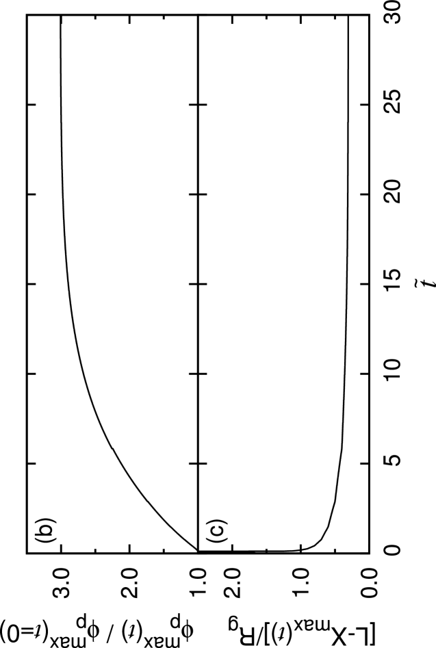
Figure 5: (a) Transient evolutions of the segment concentration profiles $\phi_{\rm{p}}(x,t)$, (b) the peak concentration, and (c) the distance from the peak position to the downstream-side wall. Applied parameters are: $\bar{\phi}_{\rm{p}}=0.1$, $N=1000$, $\chi=0.5$, $L/R_{\rm{g}}=10$, and Pe=0.05 at $\tilde{t}=t/\tau\geq 0$. The profiles are at $\tilde{t}=$0 (no flow), 1, 2, 4, 8, 16, and 32. At ${\tilde{t}}\simeq$20, the profile reaches a steady state as seen from (b) and (c). Note that the results shown in Fig.3 are based on GSA, here the profiles are calculated by using the dynamic SCFT scheme.

Figure 6: (a) Steady state volume fraction profiles of polymer segments in the polymer solution ($\bar{\phi}_{\rm{p}}=0.1$, $N=1000$, $\chi=0.5$, $L/R_{\rm{g}}=10$) at Pe= 0, 0.01, 0.03, 0.05 and 0.1. (b, c) Change of the peak concentration $\phi_{{\rm{p}}}^{\rm max}({\sf Pe})$ and the distance from the peak position $x_{\rm max}({\sf Pe})$ to the downstream-side wall for various $\sf Pe$. The data are computed by the dynamic SCFT scheme.

Figure 3 shows the transient behavior of $\phi_{\rm{p}}(x,t)$ in a slit with $L/R_{\rm{g}}=1$ after imposing a fluid flow with Pe=0.05 to an equilibrium profile at $t=0$. The time evolutions of the peak value $\phi_{{\rm{p}}}^{\rm max}(t)$ and the distance from the position $x_{\rm max}(t)$ to the downstream-side wall are shown in Fig.3(b) and (c), respectively. The shift of the peak position to the steady state position is slightly faster than that of the peak concentration, i.e., the peak position reaches steady state first, and then the concentration profile becomes sharper gradually. This indicates that a strong convective effect applies to the polymer segments and relatively slow relaxation of the polymer distribution across the slit. The time the system needs to reach the steady state is approximately 15$\tau$ to 20$\tau$ for ${\sf Pe}=0.05$, which is consistent with the accumulation time.

In Fig.4, we show that the steady state concentration profiles $\phi_{\rm{p}}(x,\infty)$ evolve upon increasing the flow rate characterized by Pe=0, 0.05, 0.1, 0.2 and 0.3 in a polymer solution with $\bar{\phi}_{\rm{p}}=0.1$, $N=1000$ and $\chi=0.5$. Figure 4(b) and (c) show the peak height $\phi_{{\rm{p}}}^{\rm max}({\sf Pe})$ of the concentration profile and the distance from the peak position $x_{\rm max}({\sf Pe})$ to the downstream-side wall at steady state under various flow strengths. The peak height $\phi_{{\rm{p}}}^{\rm max}$ increases quadratically with Pe for small $\sf Pe$ as expected in Eq.(32). In contrast to the peak height $\phi_{{\rm{p}}}^{\rm max}$, the shift of the peak position for ${\sf Pe}\hskip 3.00003pt\raisebox{1.72218pt}{$<$}\raisebox{-3.01385pt}{$\sim$}\hskip 3.00003pt0.02$ is well described by a linear approximation of Eq.(33) as seen from Fig.4(c). For ${\sf Pe}\hskip 3.00003pt\raisebox{1.72218pt}{$>$}\raisebox{-3.01385pt}{$\sim$}\hskip 3.00003pt0.02$, the shift of peak position to the downstream side is suppressed due to the wall effect. Specifically from Eq.(21), the peak position is determined by the competition of polymer segment fluxes induced by the hydrodynamic flow and by the thermodynamic force. The suppression of the peak shift distance is due to the increase of the thermodynamic flux by accumulating polymer chains at the downstream side. As seen in Fig.4(b) (and later in Fig.6(b), Fig.8(c) and Fig.10(b)), the segment volume fraction at the peak seems to increase indefinitely with Pe, while the peak position seems to saturate. This is because we restrict our study to a dilute to semi-dilute polymer solution, and we have omitted the $\phi_{\rm{s}}^{2}$-factor in the effective diffusion coefficient of eq.(21). This factor appears in the original transport equation, Eq.(8). If the volume fraction of polymer segment at the peak comes close to unity, $\phi_{\rm{s}}^{2}\rightarrow 0$, the effective diffusivity approaches zero around the peak. In such a case, however, the dilute to semi-dilute assumption is no longer valid, and the non-uniform velocity and the viscoelastic effects should be taken into account. This complicated scenario will be investigated in future work.

Figure 7: Concentration profiles of $s$-th segment in the polymer solution ($\bar{\phi}_{\rm{p}}=0.1$, $N=1000$, $\chi=0.5$, $L/R_{\rm{g}}=10$) at steady states under (a) Pe=0 (no flow) and (b) Pe=0.1 in the region $0.5\leq x\leq 1$. The lines are for $s=0$ (solid line), 0.05 (dashed), 0.2 (dash dotted) and 0.5 (dotted). The two insets in (b) show segment profiles very close to the downstream-side wall.

3.1.2 Wide Slit, $L>\pi R_{\rm{g}}$

When the distance $L$ is larger than $\pi R_{\rm{g}}$, GSA can not be used to evaluate the chemical potential difference $\mu(\vec{r})$. Here we utilize the scheme (i)-(iv) based on DSCFT explained in Sec. 2.2. To demonstrate the scheme, we consider the case of $L/R_{\rm{g}}$=10. Firstly, we show the time evolution of the concentration profiles under Pe=0.05 in Fig.5, in which the volume fraction profile of the polymer solution ($\chi=0.5$) at a quiescent state ($\sf Pe$=0) coincides with the analytical result of the depletion profile near a single wall RemcoBook2011 ; Taniguchi1992 ; Eisenriegler1996 . As $t\rightarrow\infty$, the peak appears near the end of the depletion zone along the downstream side. In comparison with the narrow slit case, $x_{\rm max}(t)$ shifts to the steady state position faster than that of the peak height (Fig.5(b) and (c)). Although this tendency has been found in the narrow slit case (Fig.3), it is enhanced in the wider slit case as seen in Fig.5. The time the system needs to reach steady state is approximately $20\tau$ as seen from Fig.5(a) and (b). The accumulation time ($t^{\ast}\sim 20\tau$) gives a better estimation for ${\sf Pe}=0.05$ than the narrow slit case described in sec.3.1.1. This good agreement is owing to the good estimation of the transport distance of the polymer segments $L$ in the accumulation time.

Figure 6 shows the steady state concentration profiles for slit width $L/R_{\rm{g}}=10$, Pe=0 to 0.1 in the polymer solution of $\bar{\phi}_{\rm{p}}=0.1$, $N=1000$ and $\chi=0.5$. These are numerical results obtained by the dynamic SCFT scheme described in Eq.(8) and Eqs.(9)-(16). In addition, the peak concentration and its position at steady state are functions of $\sf Pe$. For $\sf Pe\hskip 3.00003pt\raisebox{1.72218pt}{$>$}\raisebox{-3.01385pt}{$\sim$}\hskip 3.00003pt$ 0.05 the peak position does not change much, but the peak height continues to increase with $\sf Pe$. This indicates that the segment accumulation becomes narrower while keeping the peak position almost the same as Pe increases, which is due to the a strong depletion effect from the wall.

Figure 8: Steady state results for good solvent conditions in a narrow slit ($L/R_{\rm{g}}=1$, $\bar{\phi}_{\rm{p}}=0.1$, $N=1000$). (a) Equilibrium (Pe=0) concentration profiles of polymer segments in good solvents with $\chi=-$0.5, 0.0, 0.2, 0.3, 0.4, and in $\Theta$-solvent ($\chi=0.5$) from the bottom to the top lines near the middle point. (b) The polymer segment volume fraction profiles for $\chi=0$ and Pe=0 to 2. The peak height (c) and the distance from the peak position to the downstream-side wall (d) for $\chi$=0 (solid line), and 0.3 (dashed line) are compared with the $\Theta$-solvent ($\chi=0.5$, $m=1$, dash-dotted line) results. As a reference, the test case of $\chi=0.5$ and $m=3/4$ is shown by the dotted line. The graph of the $\Theta$-solvent is truncated at a peak height higher than 6$\bar{\phi}_{\rm{p}}$.

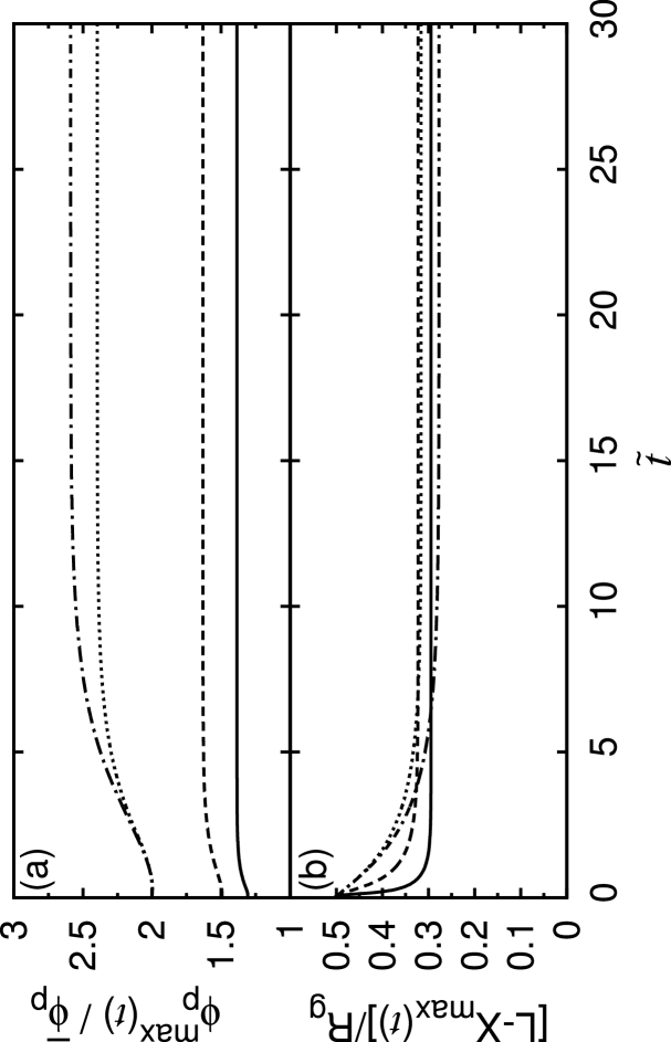
Figure 9: The time evolution of the peak concentration (a) and distance (b) from the peak position to the downstream-side wall in polymer solutions within a narrow slit ($L/R_{\rm{g}}=1$, $\bar{\phi}_{\rm{p}}=0.1$, $N=1000$) under steady flows with $\sf Pe=0.05$ for $\chi$=0 (solid line), 0.3 (dashed line), and 0.5 ($\Theta$-solvent, $m=1$, dash-dotted line). As a reference, the case of $\chi=0.5$, but with $m=3/4$ is shown by the dotted line.

The individual segment concentration provides further details of the convective effect. The statistical weight $q(x,s)$ obtained by Eq.(12) through the procedures (i)-(iv) is used to calculate the concentration profile $\phi_{\rm{p}}(s,x,t)$ for the $s$-th segment :

$$\phi_{\rm{p}}(s,x,t)={V\bar{\phi}_{\rm{p}}\over Q_{\rm{p}}}q(s,x)q(1-s,x).$$ (35)

Figure 7 shows the concentration profiles for the $s$-th segment at steady state for $s=$0.0 (end point), 0.05, 0.20, and 0.5 (midpoint) under two conditions: (a) Pe=0 (no flow) and (b) Pe=0.1. Only the region $0.5\leq x\leq 1$ is presented. The profile for Pe=0 is symmetric about $x$=0.5, and for Pe=0.1 the concentration is very low for $0\leq x\leq 0.5$. The distortion of the polymer segment concentration is significantly enhanced by the flow. Furthermore, in the case of Pe=0.1, the distribution of the end segment ($s=0$) is the broadest among others and the distributions for $0.1\hskip 3.00003pt\raisebox{1.72218pt}{$<$}\raisebox{-3.01385pt}{$\sim$}\hskip 3.00003pts<0.5$ are similar to the case of $s=0.5$ (midpoint) as expected Eisenriegler1983 ; Eisenriegler1993 ; Eisenriegler2002 .

3.2 Good-solvent cases

3.2.1 Narrow Slit, $L<\pi R_{\rm{g}}$

For good-solvent condition ($\chi<1/2$, $m=3/4$) under steady flow, the volume fraction profile can be obtained from Eq.(22). When Pe=0, we obtain the analytical volume fraction profile as (see Fig.8(a), derivation is given in Appendix A)

$$\phi_{\rm{p}}(x)=\varphi_{\rm{o}}^{2}(x)=[\varphi_{\rm m}{\rm{sn}}({\tilde{x}},k)]^{2},$$ (36)

where $\varphi_{\rm m}$ is the maximum value of $\sqrt{\phi_{\rm{p}}(x)}$, ${\rm{sn}}(\tilde{x},k)$ is the Jacobi elliptic integral, $\tilde{x}=\varphi_{\rm{m}}x\sqrt{v/2k^{2}}L/\ell$, and the constant $k$ is defined by $k^{2}={v\varphi_{\rm{m}}^{2}/[2\mu_{\rm{o}}(0)-v\varphi_{\rm{m}}^{2}]}.$ From Eq.(26) we obtain the first-order asymptotic equation under a weak flow condition (${\sf Pe}\ll 1$):

$$\biggr{[}~{}{d^{2}\over d{\tilde{x}}^{2}}+k^{2}+1-6k^{2}{\rm{sn}}^{2}({\tilde{x}},k)~{}\biggr{]}\tilde{\varphi}_{1}({\tilde{x}})=$$

$$-{L^{2}\over 4\ell^{2}K^{2}(k)}{\rm{sn}}({\tilde{x}},k)\biggr{[}\mu_{1}(0)+{\varphi_{\rm{m}}\over 2K(k)}\int_{0}^{\tilde{x}}{\rm{sn}}({\tilde{x}}^{\prime},k)d{\tilde{x}}^{\prime}\biggr{]},\quad\quad$$ (37)

where $\tilde{\varphi}_{1}=\varphi_{1}/\varphi_{\rm{m}}$. The constant $\mu_{1}(0)$ is determined by the normalization condition $\int_{0}^{1}\varphi^{2}(x)dx=1$. Unlike the $\Theta$-solvent case, analytic approximations are extremely involved here, and thus the concentration profiles are obtained numerically for both weak and strong flow conditions.

Figure 10: (a) Steady state profiles of a polymer solution ($\bar{\phi}_{\rm{p}}=0.1$, $N=1000$, and $\chi=0$) in a wide slit with $L/R_{\rm{g}}=10$ under steady flows with Pe=0, to 0.5, (b) the peak height $\phi_{{\rm{p}}}^{\rm max}({\sf Pe})$, and (c) the distance from the peak position to the downstream-side wall as a function of ${\sf Pe}$. The inset in (a) shows the result near the wall. The results are computed by using the dynamical SCFT scheme.

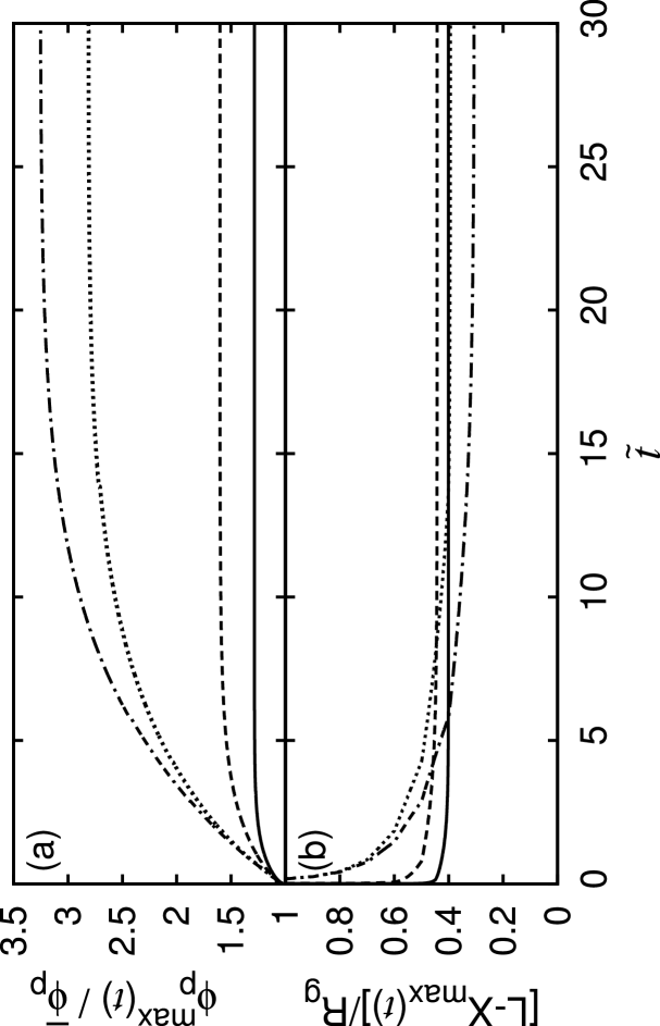
Figure 11: The time evolution of the peak concentration (a) and distance (b) from the peak position to the downstream-side wall in polymer solutions within a wide slit ($L/R_{\rm{g}}=10$, $\bar{\phi}_{\rm{p}}=0.1$, $N=1000$) under steady flows with $\sf Pe=0.05$ for $\chi$=0 (solid line), 0.3 (dashed line), and 0.5 ($\Theta$-solvent, $\chi=0.5$, $m=1$, dash-dotted line). As a reference, the case of $\chi=0.5$, but with $m=3/4$ is shown by the dotted line.

In Fig.8(b), we plot steady state volume fraction profiles $\phi_{\rm{p}}(x)$ of a polymer solution for various Pe-values. In Fig.8(c) and (d), both the peak height and position are plotted as functions of Pe for various $\chi$-values. As a reference, the $\Theta$-solvent ($\chi=0.5$, $m=1$) result given in Fig.4 is shown by the dash-dotted lines, and the case of $\chi=0.5$ and $m=3/4$ is shown by the dotted line. From the comparison among the cases of $\chi=0$, 0.3, and 0.5 with $m$=3/4 in Fig.8(c), we find that the peak height of polymers concentration in a good solvent is less-sensitive to the convective effect with lower $\chi$. This is caused by the enhanced excluded volume effect for better solvency. On the other hand, the behaviors of the peak height in the $\Theta$-solvent are slightly different from those in good-solvent conditions. The different behavior between the good- and $\Theta$-solvents comes from the $\phi_{\rm{p}}$-dependent diffusion coefficient in Eq.(21). This can be confirmed from the evidence that the peak position for $\chi=0.5$ but with $m=3/4$ exhibits a similar ${\sf Pe}$-dependence to those in good solvents where $m=3/4$.

Figure 9 shows that a polymer solution with smaller $\chi$ exhibits a smaller peak height and reaches steady state faster. When $\chi=0$, only a small change of peak height appears due to the larger excluded volume effect under a better solvency. However, the distance between the peak position and the wall on the downstream side for $\chi=$0.3 is larger than those in $\chi=0.0$ and $\chi=0.5$. The reason is because that the depletion thickness in $\chi=0$ is smaller than those of $\chi=0.3$ in a quiescent state Fleer2003 , and therefore under a flow, initially the peak is formed at a position relatively closer to the wall for $\chi=0$.

Although the depletion thickness at a quiescent state for $\chi=0.5$ is larger than for $\chi=0.3$, the peak can easily be shifted by the flow compared to the two good solvent cases, and therefore the peak position becomes closer to the wall for $\chi=0.5$ than for the $\chi=0.3$ case. As seen in Fig.9, under a good solvent condition, the time for systems to reach the steady state under ${\sf Pe}=0.05$ is approximately $2\tau$ for $\chi=0$ and $3\tau$ for $\chi=0.3$, which are much shorter than the estimated accumulation time ($t^{\ast}\sim 20\tau$) due to the excluded volume effect.

3.2.2 Wide Slit, $L/R_{\rm{g}}=10$

Figure 10 shows the results for the same polymer solution in a wide slit with $L/R_{\rm{g}}=10$ and $0\leq{\sf Pe}\leq 0.5$. The steady state profiles of polymer segment volume fraction under various $\sf Pe$ are shown in (a). The peak concentration and position are plotted in Figures (b) and (c). As seen from (a) and (c), the profile is almost flat in the quiescent state and by applying a flow the peak position jumps from the center of the slit to a downstream position near the wall. The polymer segment profile is strongly influenced by the applied flow. Because the depletion thickness under good solvent conditions is relatively small compared to the slit width, the profile has a sharp peak. This is also because the depletion thickness is reduced due to good solvency or large excluded volume effect among the polymer chains.

Figure 11 shows that the concentration profiles in good solvents reach steady states much faster than in a $\Theta$-solvent, similar to the good solvent case shown in Fig.9. The shorter accumulation time comes from a smaller depletion thickness for a better solvency at the quiescent state, such that the peak appears at the very end of depletion zone. As a result, the accumulation time is much smaller than the estimated one.

Figure 12: Effect of slit width. (a) The peak volume fraction and (b) the distance from the peak position to the wall in the downstream side in polymer solutions ($\bar{\phi}_{\rm{p}}=0.1$, $N=1000$) at steady states under a flow with $\sf Pe=0.05$ for $\chi$=0 (solid line), 0.3 (dashed line), the $\Theta$-solvent case ($\chi=0.5,m=1$) (dash-dotted line), and the case with $\chi=0.5$ and $m=3/4$ (dotted line).

In Fig.12 we demonstrate the dependency of the slit width for ${\sf Pe}=0.05$ under solvent conditions $\chi=$0.0, 0.3 and 0.5. The peak concentrations $\phi_{\rm{p}}^{\rm max}(L)$ for the given $\chi$-values are not sensitive to $L/R_{\rm{g}}$. In a $\Theta$-solvent ($\chi=0.5$, $m$=1) and the test case with $\chi=0.5$ and $m=3/4$, the peak concentrations increase somewhat with $L$. In good solvents, however, the peaks slightly decrease with increasing $L$. Under a flow condition, the polymer segment accumulation is determined by the competition between the hydrodynamic flux and the diffusive thermodynamic flux. The thermodynamic flux is contributed by the excluded volume effect and the translational entropy that suppresses the polymer segment accumulation at the downstream side. The increase of the peak concentration in a $\Theta$-solvent might come from rather weak excluded volume effect. In good solvents, the excluded volume effect lowers the peak height and the translational entropy also suppresses the accumulation when the slit width becomes large ($L\gg R_{\rm{g}}$). As seen from Fig.12(b), the distance between the peak position and the downstream-side wall slightly increases with $L$ for all the $\chi$-values under a fixed ${\sf Pe}$. In the range of $1\leq L/R_{\rm{g}}\leq$10, the distance is roughly less than $0.1R_{\rm{g}}$ for $\chi=$0.0, 0.3 and 0.5, which means that the depletion thickness in a flow field is mainly determined by ${\sf Pe}$. Irrespective of the slit width, a better solvency always exhibits a weaker polymer segment accumulation because of the larger exclude volume effect. On the other hand, the shift distance is larger for $\chi=$0.3 than for the $\chi=0.0$ and $\chi=0.5$ cases due to the same reason explained when discussing Fig.9.

Finally, because we used DSCFT scheme to obtain steady state results for $L/R_{\rm{g}}>1$, the computational expense is much higher than for the $L/R_{\rm{g}}=1$ case using GSA, which makes it difficult to reach sufficient accuracy for $L\gg R_{\rm{g}}$. The distance between the peak position and the wall at the steady state slightly increases with $L$ as seen in Fig.12(b), we conclude that the distance is almost constant against $L$ and there is no clear physical reason why the distance should increase with $L$ for fixed $\sf Pe$.

4 Conclusions

The two-fluid model and the dynamic self-consistent field theory are successfully combined to characterize the polymer segment dynamics under the influence of a uniform flow and polymer depletion effect. This conceptual model demonstrates the segment concentration profile of a polymer solution ($0\leq\chi\leq 0.5$) confined in between two parallel and solvent permeable walls. The continuous concentration profiles in transient and steady state analysis are characterized by the Peclet number Pe, excluded volume parameter $\nu$, and the slit width $L/R_{\rm{g}}$. The polymer segments accumulate at the downstream due to the convective effect. The competition between the hydrodynamic flux and the diffusive thermodynamic flux are featured by the height and position of the concentration peak. The mean flow transports polymer segments to the downstream and the thermodynamic flux acts to minimize the concentration gradient in bulk and imposes a depletion region near the walls to suppress the loss of conformation entropy of the polymer chains. We provide analytical ground state approximation of the concentration profiles for the steady state and narrow slit case under a weak flow with theta or good solvents. All wide slit cases in either weak or strong flow are resolved numerically using the dynamic self-consistent field theory to distinguish the individual segment-level profiles influenced by the flow.

Using DSCFT, we find that the distribution of the end segment is the broadest as compared to other segments that tend to follow the distribution of the center-of-mass segments. At steady state, regardless the slit width, the peak concentration in a good solvent is less sensitive to the flow effect with decreasing $\chi$. This is due to the strong excluded volume effect in the good solvent. Such behavior does not appear in the theta-solvent case because the $\phi_{\rm{p}}$-dependent diffusion coefficient vanishes. The peak concentration and its location are mainly determined by the flow strength and the excluded volume effect, and weakly depend on the slit width. In transient analysis, we characterize the accumulation time for both narrow and wide slits. Regardless the solvent condition and the slit width, the peak location responses faster and reaches steady state earlier than the peak height. The estimated accumulation time is best applicable for the theta solvent, but is somewhat over-estimated for good solvents due to the small peak shift owing to the excluded volume effect. In summary, the theoretical model has revealed the transient relaxation and steady state features of the convective depletion dynamics of polymer solutions. It will be interesting to extend this model to higher-dimensional cases and validate the findings experimentally in the future.

Appendix A Equilibrium Profile in Good Solvents

The equilibrium profile of polymer chains in a good solvent is described by Eq.(25). Multiplying Eq.(25) by $d\varphi_{\rm{o}}/dx$ and then integrating it once, we obtain

$${\ell^{2}\over 2L^{2}}\Bigr{(}{d\varphi_{\rm{o}}\over d{x}}\Bigr{)}^{2}+{1\over 2}\mu_{\rm{o}}(0)\varphi_{\rm{o}}^{2}-{1\over 4}v\varphi_{\rm{o}}^{4}=C,$$ (38)

where $v=(1-2\chi)\bar{\phi}_{\rm{p}}$, the constant $C=\varphi_{\rm m}^{2}\mu_{\rm{p}}(0)/2-\varphi_{\rm m}^{4}{v}/4$ is determined by $d\varphi_{\rm{o}}/dx|_{x=1/2}=0$ and $\varphi_{\rm{o}}(1/2)=\varphi_{\rm m}$ at the middle point. Therefore, Eq.(38) becomes

$$\biggr{(}{d\tilde{\varphi}_{\rm{o}}\over d{{{\tilde{x}}}}}\biggr{)}^{2}=(1-\tilde{\varphi}_{\rm{o}}^{2})(1-k^{2}\tilde{\varphi}_{\rm{o}}^{2}),$$ (39)

where $\tilde{\varphi}_{\rm{o}}\equiv\varphi_{\rm{o}}/\varphi_{\rm m}$, $\tilde{x}=x\varphi_{\rm{m}}\sqrt{vL^{2}/2k^{2}\ell^{2}}$, and $k^{2}$ is defined as

$$k^{2}={v\over 2\mu_{\rm{o}}(0)/\varphi_{\rm{m}}^{2}-v}.$$ (40)

Integrating Eq.(39) yields

$$\tilde{\varphi}_{\rm{o}}({\tilde{x}})={\rm{sn}}({\tilde{x}},k),$$ (41)

where ${\rm{sn}}(x,k)$ is the Jacobi elliptic integral. From $\tilde{\varphi}_{\rm{o}}=1$ at $x=1/2$ we find

$$\varphi_{\rm{m}}={2\ell K(k)\over L}\sqrt{2k^{2}\over v},$$ (42)

where $K(k)$ is the complete elliptic integral defined as

$$K(k)=\int_{0}^{1}{dt\over\sqrt{(1-t^{2})(1-k^{2}t^{2})}}.$$ (43)

From the normalization condition $\int_{0}^{1/2}\phi_{\rm{o}}(x)dx=1/2$, we have

$${8k^{2}\ell^{2}K(k)\over vL^{2}}\int_{0}^{K(k)}{\rm{sn}}^{2}({\tilde{x}},k)d{\tilde{x}}=1.$$ (44)

Based on the properties of elliptic integrals it follows

$$K(k)\bigr{[}K(k)-E(k)\bigr{]}={vL^{2}\over 8\ell^{2}},$$ (45)

where $E(k)$ is the second kind complete elliptic integral, expressed as

$$E(k)=\int_{0}^{\pi/2}\sqrt{1-k^{2}\sin^{2}\varphi~{}}~{}d\varphi.$$ (46)

From Eqs.(40) and (42) we obtain

$$\mu_{\rm{o}}(0)={4\ell^{2}K^{2}(k)\over L^{2}}(k^{2}+1).$$ (47)

In summary, for a given $v$ and $L$ we can determine $k$ from Eq.(45), and then evaluate $\varphi_{\rm m}$ and $\mu_{\rm{o}}(0)$ from (42) and (47), respectively.

References

- (1) G.J. Fleer, M.A. Cohen Stuart, J.M.H.M. Scheutjens, T. Cosgrove, and B. Vincent. Polymers at Interfaces. (Chapman and Hall, New York, 1993).
- (2) E. Eisenriegler, J. Chem. Phys. 79, (1983) 1052.
- (3) A. Hanke, E. Eisenriegler, and S. Dietrich, Phys. Rev. E 59, (1999) 6853.
- (4) G.J. Fleer and R. Tuinier, Adv. Colloid Interface Sci. 143, (2008) 1.
- (5) P.G. De Gennes, Scaling Concepts in Polymer Physics (Cornell University Press, Ithaca, 1979).
- (6) G.J. Fleer, A.M. Skvortsov, and R. Tuinier, Macromolecules 36, (2003) 7857.
- (7) G.J. Fleer, A.M. Skvortsov, and R. Tuinier, Macromol. Theory Sim. 16, (2007) 531 .
- (8) S. Asakura and F. Oosawa, J. Chem. Phys. 22, (1954) 1255.
- (9) A. Vrij, Pure Appl. Chem. 48, (1976) 471.
- (10) R. Verma, J.C. Crocker, T.C. Lubensky, and A.G. Yodh, Macromolecules 33, (2000) 177.
- (11) H.N.W. Lekkerkerker, W.C.K. Poon, P.N. Pusey, A. Stroobants, and P. B. Warren, Europhys. Lett. 20, (1992) 559.
- (12) S. M. Ilett, A. Orrock, W. C. K. Poon, and P. N. Pusey, Phys. Rev. E 51, (1995) 1344 .
- (13) E. J. Meijer and D. Frenkel, J. Chem. Phys. 100, (1994) 6873.
- (14) R. Tuinier, P.A. Smith, W.C.K. Poon, S.U. Egelhaaf, D.G.A.L. Aarts, H.N.W. Lekkerkerker, and G.J. Fleer, Europhys. Lett. 82, (2008) 68002.
- (15) R. Tuinier and T. Taniguchi, J. Phys: Condens. Matter L9, (2005) 17.
- (16) E. Duering and Y. Rabin, Macromolecules 23, (1990) 2232.
- (17) R. Tuinier, J. K. G. Dhont, and T.-H. Fan, Europhys. Lett. 75, (2006) 929.
- (18) T.-H. Fan, J. K. G. Dhont, and R. Tuinier, Phys. Rev. E 75, (2007) 011803.
- (19) T.-H. Fan, R. Tuinier, Soft Matter 6, (2010) 647.
- (20) T. Odijk, Physica A 337, (2004) 389.
- (21) M. Doi and A. Onuki, J. Phys. II France 2, (1992) 1631.
- (22) D. M. Hall, T. Lookman, G. H. Fredrickson and S. Banerjee, J. Comp. Phys. 244, (2007) 681.
- (23) H. Pasch and B. Trathnigg, HPLC of polymers, (Springer, Berlin, Heidelberg, New, York, 1997), L. R. Snyder J. J. Kirkland, Introduction to modern liquid chromatography (Wiley, NY, 1979).
- (24) H. Tanaka, Phys. Rev. Lett. 71, (1996) 3158-3161 . H. Tanaka, J. Phys. Cond. Matt. 12, (2000) R207-264, M. Takenaka, H. Takeno, T. Hashimoto and M. Nagao, J. Chem. Phys. 124, (2006) 104904, N. Toyoda, M. Takenaka, S. Saito and T. Hashimoto, Polymer 42 (2001) 9193, M. Takenaka, H. Takeno, H. Hasegawa, S. Saito, T. Hashimoto and M. Nagao, Phys. Rev. E 65, (2002) 021806.
- (25) T. Imaeda, A. Furukawa and A.Onuki, Phys. Rev. E 70, (2004) 051503, T. Taniguchi and A. Onuki, Phys. Rev. Lett. 77, (1996) 4910.
- (26) E. Helfand and G.H. Fredrickson, Phys. Rev. Lett. 62, (1989) 2468, S. T. Milner, Phys. Rev. E 48, (1993) 3674.
- (27) M. Koga, M. Takenaka, T. Hashimoto, T. Inoue, and H. Watanabe J. Chem. Phys. 126, (2008) 164911.
- (28) H. N. W. Lekkerkerker and R. Tuinier, Colloids and the Depletion Interaction, (Springer, Heidelberg 2011).
- (29) A. A. Louis, P. G. Bolhuis, E. J. Meijer, and J. P. Hansen, J. Chem. Phys. 116, (2002) 10547.
- (30) G. H. Fredrickson, The Equilibrium Theory of Inhomogeneous Polymers, (Clarendon press, Oxford, 2006).
- (31) T. Taniguchi, T. Kawakatsu and K. Kawasaki, AIP conference proceedings 256, (1992) 503.
- (32) E. Eisenriegler, A. Hanke and S. Dietrich, J. Chem. Phys., 54, 1134 (1996).
- (33) E. Eisenriegler, Polymers near Surfaces, (World Scientific, Singapore 1993).
- (34) E. Eisenriegler, J. Chem. Phys., 116, 449 (2002).