Expansion Coding: Achieving the Capacity of an AEN Channel

Abstract

A general method of coding over expansions is proposed, which allows one to reduce the highly non-trivial problem of coding over continuous channels to a much simpler discrete ones. More specifically, the focus is on the additive exponential noise (AEN) channel, for which the (binary) expansion of the (exponential) noise random variable is considered. It is shown that each of the random variables in the expansion corresponds to independent Bernoulli random variables. Thus, each of the expansion levels (of the underlying channel) corresponds to a binary symmetric channel (BSC), and the coding problem is reduced to coding over these parallel channels while satisfying the channel input constraint. This optimization formulation is stated as the achievable rate result, for which a specific choice of input distribution is shown to achieve a rate which is arbitrarily close to the channel capacity in the high SNR regime. Remarkably, the scheme allows for low-complexity capacity-achieving codes for AEN channels, using the codes that are originally designed for BSCs. Extensions to different channel models and applications to other coding problems are discussed.

I Introduction

In this work, we propose the method of constructing (binary) expansions of discrete-time continuous alphabet channels, and coding over the resulting set of parallel channels. We apply this coding over expansions method to additive exponential noise (AEN) channels, where the signal and noise terms constructing the channel output are represented with their corresponding binary digits. Focusing on the additive exponential noise component, we show that the binary expansion of the noise consists of independent Bernoulli distributed random variables at each level. (The mean of each random variable is a function of their level number in the expansion and the mean of the underlying exponential noise.) This way, thanks to the expansion technique, we show that continuous alphabet channels can be considered as a set of parallel binary symmetric channels (BSCs).

Instead of coding for every level in the expansion, we consider signaling over a finite number of levels, and we resolve the problem arising from carryovers either by considering them as noise, or by decoding them the least significant bit onwards to the most significant bit. For each case, we state the corresponding achievable rate as an optimization problem, where the rate is maximized over the choices of the Bernoulli distributions for the signal transmission over each level with the constraint that that the combined random variables satisfy the channel input constraint. Then, utilizing an approximately optimal input distribution, we show that one can celebrate the achievability of an $\epsilon$-gap to capacity result in the high SNR regime. This method together with capacity-achieving low-complexity codes (such as polar coding) allows one to achieve the capacity of the AEN in the high SNR regime.

The additive exponential noise (AEN) channel is of particular interest as it models worst-case noise given a mean and a non-negativity constraint on noise [1]. In addition, the AEN model naturally arises in non-coherent communication settings, and in optical communication scenarios. (We refer to [1] and [2] for an extensive discussion on the AEN channel.) Verdú derived the optimal input distribution and the capacity of the AEN channel in [1]. Martinez, on the other hand, proposed the pulse energy modulation scheme, which can be seen as a generalization of amplitude modulation for the Gaussian channels. In this scheme, the constellation symbols are chosen as $c(i-1)^{l}$, for $i=1,\cdots,2^{M}$ with a constant $c$, and it is shown that the information rates obtained from this constellation can achieve an energy (SNR) loss of $0.76$ dB (with the best choice of $l=\frac{1}{2}(1+\sqrt{5})$) compared to the capacity in the high SNR regime. Another constellation technique for this coded modulation approach is recently considered in [3], where it is shown that log constellations are designed such that the real line is divided into ($2M-1$) equally probable intervals. $M$ of the centroids of these intervals are chosen as constellation points, and, by a numerical computation of the mutual information, it is shown that these constellations can achieve within a $0.12$ dB SNR gap in the high SNR regime. Our approach, which achieves arbitrarily close to the capacity of the channel, outperforms these previously proposed modulation techniques.

The rest of the paper is organized as follows. The next section describes the AEN channel model. In Section III, we present the key Lemma which shows that one independent Bernoulli distributed random variables occur in the binary expansion of an exponential random variable. Armed with this result, Section IV develops the expansion modulation technique, where we state the main results of the paper. Numerical results are provided in Section IV-C, and the paper concludes with a discussion section (Section V).

II Channel model and background

We consider the additive exponential noise (AEN) channel given by

$$Y_{i}=X_{i}+N_{i},i=1,\cdots,n,$$ (1)

where $N_{i}$ are independently and identically distributed according to the additive noise with an exponential density with mean $E_{N}$; i.e., omitting the index $i$, the noise has the following density:

$$\textrm{Pr}\{N=n\}=\frac{1}{E_{N}}e^{-\frac{n}{E_{N}}}u(n),$$ (2)

where $u(n)=1$ for $n\geq 0$ and $u(n)=0$ otherwise.

The transmitter conveys one of the messages, $m$, which is uniformly distributed in ${\cal M}$, i.e., the random message $m\in{\cal M}\triangleq\{1,\cdots,2^{nR}\}$; and it does so by mapping the message to the channel input using the encoding function $f(\cdot):{\cal M}\to{\cal X}^{n}$, where $X_{1}^{n}(m)=f(m)$, under the constraints that ${\cal X}=\Re$ and

$$\frac{1}{n}\mbox{\bb E}\big{[}\sum\limits_{i=1}^{n}X_{i}\big{]}\leq E_{X},$$ (3)

where $E_{X}$ is the maximum average energy.

The decoder uses the decoding function $g(\cdot)$ to map its channel observations to an estimate of the message. Specifically, $g(\cdot):{\cal Y}^{n}\to{\cal M}$, where the estimate is denoted by $\hat{M}\triangleq g(Y^{n})$.

The rate $R$ is said to be achievable, if the average probability of error defined by

$$P_{e}\triangleq\frac{1}{|{\cal M}|}\sum\limits_{m\in{\cal M}}\textrm{Pr}\{g(Y^{n})\neq m|m\textrm{ is sent. }\}$$ (4)

can be made small for large $n$. The capacity of AEN is denoted by $C$, which is the maximum achievable rate $R$.

The capacity of AEN is given by [1], where

$$C=\log(1+\textrm{SNR}),$$ (5)

where $\textrm{SNR}=\frac{E_{X}}{E_{N}}$, and the capacity achieving input distribution is given by

$$p^{*}(x)=\left(\frac{E_{X}}{(E_{X}+E_{N})^{2}}e^{\frac{-x}{E_{X}+E_{N}}}+\frac{E_{N}}{(E_{X}+E_{N})}\delta(x)\right)u(x),$$ (6)

where $\delta(x)=1$ if $x=0$, and $0$ otherwise. Note that this is the $p^{*}(x)=\arg\max\limits_{p(x)}I(X;Y)$, where $p(y|x)$ is given by the AEN channel (1).

Surprisingly, while the capacity achieving input distribution for the additive white Gaussian noise (AWGN) channel is Gaussian, here the optimal input distribution is not exponentially distributed. However, we observe that in the high SNR regime, the optimal distribution gets closer to an exponential distribution with mean $E_{X}+E_{N}$.

III Exponential Distribution: Binary Expansion

We show the following lemma, which allows us to have independent Bernoulli random variables in the binary expansion of an exponential random variable.

Lemma 1

Let $B_{l}$’s be independent Bernoulli random variables with parameters given by $p_{l}$, i.e., $\textrm{Pr}\{B_{l}=1\}=p_{l}$ and $\textrm{Pr}\{B_{l}=0\}=1-p_{l}$, and consider the random variable defined by

$$B=\sum\limits_{l=-\infty}^{\infty}2^{l}B_{l}.$$ (7)

Then, the choice of

$$p_{l}=\frac{1}{1+e^{\lambda 2^{l}}},$$ (8)

implies that the random variable $B$ is exponentially distributed with mean $\lambda^{-1}$, i.e.,

$$\textrm{Pr}\{B=b\}=\lambda e^{-\lambda b}u(b).$$ (9)

Proof:

The proof follows by extending the one given in [4]. We show the result by calculating the moment generating function of $B$. Using the assumption that $\{B_{l}\}_{l\in\mathbb{Z}}$ are mutually independent, we have

$$M_{B}(t)=\mbox{\bb E}[e^{tB}]=\mbox{\bb E}\left[e^{t\sum\limits_{l=-\infty}^{\infty}2^{l}B_{l}}\right]=\prod_{l=-\infty}^{\infty}\mbox{\bb E}\left[e^{t2^{l}B_{l}}\right].$$ (10)

Note that for any $l\in\mathbb{Z}$,

$$\mbox{\bb E}\left[e^{t2^{l}B_{l}}\right] = \frac{e^{t2^{l}}}{1+e^{\lambda 2^{l}}}+\left(1-\frac{1}{1+e^{\lambda 2^{l}}}\right)=\frac{e^{t2^{l}}+e^{\lambda 2^{l}}}{1+e^{\lambda 2^{l}}}$$ (11)

$$= \frac{1+e^{(t-\lambda)2^{l}}}{1+e^{-\lambda 2^{l}}}.$$

Then, using the fact that for any constant $\alpha\in\mathbb{R}$,

$$\prod_{l=0}^{n}(1+e^{\alpha 2^{l}})=\frac{1-e^{2^{n+1}\alpha}}{1-e^{\alpha}},$$ (12)

we can obtain the following for $t<\lambda$,

$$\prod_{l=0}^{\infty}\mbox{\bb E}\left[e^{t2^{l}B_{l}}\right] = \lim_{n\rightarrow\infty}\prod_{i=0}^{n}\frac{1+e^{(t-\lambda)2^{l}}}{1+e^{-\lambda 2^{l}}}$$ (13)

$$= \frac{1-e^{-\lambda}}{1-e^{t-\lambda}}$$

$$= \lim_{n\rightarrow\infty}\frac{1-e^{(t-\lambda)2^{n+1}}}{1-e^{t-\lambda}}\frac{1-e^{-\lambda}}{1-e^{-\lambda 2^{n+1}}}$$

$$= \frac{1-e^{-\lambda}}{1-e^{t-\lambda}}.$$

And, similarly, for the negative part, we have

$$\prod_{l=-n}^{-1}(1+e^{\alpha 2^{l}})=\frac{1-e^{\alpha}}{1-e^{\alpha 2^{-n}}},$$ (14)

which further implies that

$$\prod_{i=-\infty}^{-1}\mbox{\bb E}\left[e^{t2^{i}B_{l}}\right] = \lim_{n\rightarrow\infty}\frac{1-e^{t-\lambda}}{1-e^{(t-\lambda)2^{-n}}}\frac{1-e^{-\lambda 2^{-n}}}{1-e^{-\lambda}}$$ (15)

$$= \frac{\lambda(1-e^{t-\lambda})}{(\lambda-t)(1-e^{-\lambda})}.$$

Thus, finally for any $t<\lambda$, multiplying equations 13 and 15, we get

$$M_{B}(t) = \frac{\lambda}{\lambda-t}.$$ (16)

The observation that this is the moment generation function for an exponentially distributed random variable with parameter $\lambda$ concludes the proof. ∎

IV Modulation with expansions

Our proposed coding scheme consists of coding over expansion, referred to as expansion modulation (EM), and coding for the resulting parallel binary symmetric channels (BSCs). More specifically, EM refers to a modulation over the binary expansion of the channel over levels ranging from $-L_{1}$ to $L_{2}$, i.e.,

$$Y_{i}\triangleq\sum\limits_{l=-L_{1}}^{L_{2}}2^{l}Y_{i,l}=\sum\limits_{l=-L_{1}}^{L_{2}}2^{l}(X_{i,l}+N_{i,l}),$$ (17)

where the expansions of the signal and noise are given by

$$X_{i}\triangleq\sum\limits_{l=-L_{1}}^{L_{2}}2^{l}X_{i,l},\quad\textrm{ and }N_{i}\triangleq\sum\limits_{l=-L_{1}}^{L_{2}}2^{l}N_{i,l}.$$ (18)

When we take the limit $L_{1},L_{2}\to\infty$, the channel given by (17) corresponds to the one given by (1).

We propose coding over the expansion levels of this channel. More specifically, the least significant bit channel is given by

$$Y_{i,-L_{1}}=X_{i,-L_{1}}\oplus N_{i,-L_{1}},i=1,\cdots N.$$ (19)

A capacity achieving BSC code is utilized over this channel with input probability distribution given by $p_{-L_{1}}$. (For example, the polar coding method [5], allows one to construct capacity achieving codes for the $l=-L_{1}$ level channel.) Instead of directly using the capacity achieving code design, we use the combination of the capacity achieving code and the method of Gallager [6] to achieve a rate corresponding to the one obtained by the mutual information $I(X_{l};Y_{l})$ evaluated with an input distribution Bernoulli with parameter $p_{l}$.(The desired distributions will be made clear in the following part.)

Noting that the sum is a modulo-$2$ sum in the above channel, there will be carryovers from this sum to the next level, $l=-L_{1}+1$. Denoting the carryover seen at level $l$ as $C_{i,l}$, the remaining channels can be represented with with the following

$$Y_{i,l}=X_{i,l}\oplus\tilde{N}_{i,l},\quad i=1,\cdots n,$$ (20)

where the effective noise, $\tilde{N}_{i,l}$, is a Bernoulli random variable obtained by the convolution of the noise and the carryover $\tilde{q}_{l}\triangleq\textrm{Pr}\{\tilde{N}_{i,l}=1\}=q_{l}\otimes c_{l}\triangleq q_{l}(1-c_{l})+c_{l}(1-q_{l})$ with $q_{l}\triangleq\textrm{Pr}\{N_{i,l}=1\}$ and $c_{l}\triangleq\textrm{Pr}\{C_{i,l}=1\}$. Here, the carry over probability is given by

$$c_{l}=p_{l-1}\tilde{q}_{l-1},l\in\{-L_{1}+1,\cdots,L_{2}\}.$$ (21)

Due to Lemma 1, the noise seen at each level will be described by independent Bernoulli random variables, and therefore, our coding scheme will be over the parallel channels given by (20) for $l=-L_{1},\cdots,L_{2}$, where $\tilde{q}_{l}\triangleq\textrm{Pr}\{\tilde{N}_{i,l}=1\}=q_{l}\otimes(p_{l-1}\tilde{q}_{l-1})$.

IV-A Considering carryovers as noise

Using a capacity achieving code for BSCs, combined with the Gallager’s method, expansion modulation readily achieves the following result.

Theorem 2

Expansion modulation, when implemented with capacity achieving codes for the resulting BSCs, achieves the rate given by

$$R_{1}=\sum\limits_{-L_{1}}^{L_{2}}H(p_{l}\otimes\tilde{q}_{l})-H(\tilde{q}_{l}),$$ (22)

for any $L_{1},L_{2}>0$, where $\tilde{q}_{l}=q_{l}\otimes(p_{l-1}\tilde{q}_{l-1})$ for $l>-L_{1}$. To satisfy the energy constraint, $p_{l}\in[0,0.5]$ is chosen such that

$$\frac{1}{n}\mbox{\bb E}\left[\sum\limits_{i=1}^{n}X_{i}\right]=\frac{1}{n}\sum\limits_{i=1}^{n}\sum\limits_{l=-L_{1}}^{L_{2}}2^{l}p_{l}\leq E_{X}.$$ (23)

The optimization problem stated in the result above is highly non-trivial. However, utilizing the optimal input distribution, (6), one can adopt the following approximate distributions in Theorem 2. At a high SNR, we observe that the optimal input distribution is approximated by an exponential distribution. Then, one can simply choose $p_{l}$ from the binary expansion of the exponential distribution with mean $E_{X}+E_{N}$. To satisfy the power constraint, we use coding only for $\frac{E_{X}}{E_{X}+E_{N}}$ of the time, and for the rest we set the channel input to $0$. (As a second approach, in the numerical results, we compare this choice with the one of choosing $p_{l}$ from the binary expansion of the exponential distribution with mean $E_{X}$.) The next method gives a better rate result with a minimal increase in complexity.

IV-B Decoding carryovers

In the scheme above, let us consider decoding starting from the level $l=-L_{1}$. The receiver will obtain the correct $X_{i,-L_{1}}$ for $i=1,\cdots,n$. As the receiver has the knowledge of $Y_{i,-L_{1}}$ for $i=1,\cdots,n$, it will also have the knowledge of the correct noise sequence $N_{i,-L_{1}}$ for $i=1,\cdots,N$. With this knowledge, the receiver can directly obtain $C_{i,-L_{1}+1}$ for $i=1,\cdots,N$, which is the carryover from level $l=-L_{1}$ to level $l=-L_{1}+1$. Using this carryover sequence in decoding at level $l=-L_{1}+1$, the receiver can get rid of carryover noise. Thus, the effective channel that the receiver will see can be represented by

$$Y_{i,l}=X_{i,l}\oplus N_{i,l},\quad i=1,\cdots,n,$$ (24)

for $l=-L_{1},\cdots,L_{2}$. We remark that with this decoding strategy the effective channels will no longer be a set of independent parallel channels, as decoding in one level affects the channels at higher levels. However, if the utilized coding method is strong enough (e.g., if the error probability decays to $0$ exponentially with $n$), then this carryover decoding error can be made insignificant by increasing $n$ for a given number of levels (here, $L_{1}+L_{2}+1$). We state the rate resulting from this approach.

Theorem 3

Expansion modulation, by decoding the carryovers, achieves the rate given by

$$R_{2}=\sum\limits_{-L_{1}}^{L_{2}}H(p_{l}\otimes q_{l})-H(q_{l}),$$ (25)

for any $L_{1},L_{2}>0$, where $p_{l}\in[0,0.5]$ is chosen to satisfy

$$\frac{1}{n}\mbox{\bb E}\big{[}\sum\limits_{i=1}^{n}X_{i}\big{]}=\frac{1}{n}\sum\limits_{i=1}^{n}\sum\limits_{l=-L_{1}}^{L_{2}}2^{l}p_{l}\leq E_{X}.$$ (26)

Compared to the previous case, the optimization problem is simpler here as the rate expression is simply the sum of the rates obtained from a set of parallel channels.

We now show that the proposed scheme achieves the capacity of AEN channel in the high SNR regime for a sufficiently high number of levels. Towards this end, we provide a bound for the capacity gap, $\Delta C\triangleq C-\hat{C}$, where

$$\hat{C}=\frac{\textrm{SNR}}{1+\textrm{SNR}}\sum_{l=-L}^{L+\gamma}\left[H(p_{l}\otimes q_{l})-H(q_{l})\right]$$ (27)

is the achievable rate given in Theorem 3 with $L_{1}=L$, $L_{2}=\gamma+L$, and $\gamma=\log(1+\textrm{SNR})$, when the approximate input distribution discussed above (i.e., exponential with mean $E_{X}+E_{N}$) is used. First, we obtain the asymptotic behavior of entropy at each level.

Lemma 4

Entropy of the Bernoulli random variable at level $l$, $H(q_{l})$, is bounded by

$$H(q_{l})<c_{1}\cdot 2^{-l}\quad\;\;\;\;\text{for }\;l\geq 0,$$ (28)

$$H(q_{l})>1-c_{2}\cdot 2^{l}\quad\text{for }\;l\leq 0,$$ (29)

where $c_{1}$ and $c_{2}$ are both constants taking the values $c_{1}=3\log e$ and $c_{2}=\log e$.

Proof:

Note that,

$$H(q_{l}) =-q_{l}\log q_{l}-(1-q_{l})\log(1-q_{l})$$

$$=-\frac{1}{1+e^{2^{l}}}\log\frac{1}{1+e^{2^{l}}}-\frac{e^{2^{l}}}{1+e^{2^{l}}}\log\frac{e^{2^{l}}}{1+e^{2^{l}}}.$$

When $l\leq 0$, we obtain a lower bound as

$$H(q_{l}) =\log\left(1+e^{2^{l}}\right)-\frac{e^{2^{l}}}{1+e^{2^{l}}}\log e\cdot 2^{l}$$

$$>\log(1+1)-\log e\cdot 2^{l}$$

$$=1-\log e\cdot 2^{l}.$$

On the other hand, when $l\geq 0$, by using the facts that $\log(1+x)<\log e\cdot x$ for any $0<x<1$, and $e^{x}>1+x+x^{2}/2$ for any $x>0$, we have

$$H(q_{l}) =\frac{1}{1+e^{2^{l}}}\log\left(1+e^{2^{l}}\right)+\frac{e^{2^{l}}}{1+e^{2^{l}}}\log\left(1+e^{-2^{l}}\right)$$

$$<\frac{1}{1+e^{2^{l}}}\log\left(2e^{2^{l}}\right)+\log\left(1+e^{-2^{l}}\right)$$

$$<\frac{1+2^{l}\log e}{1+e^{2^{l}}}+e^{-2^{l}}\log e$$

$$<\frac{1+2^{l}\log e}{1+1+2^{l}+2^{2l}/2}+\frac{1}{1+2^{l}}\log e$$

$$<2^{-l}2\log e+2^{-l}\log e$$

$$=2^{-l}3\log e.$$

∎

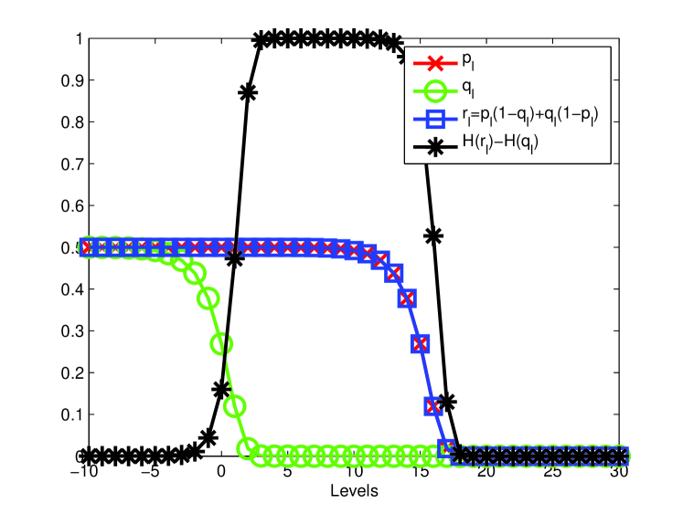
Figure 1: Signal and noise probabilities, and rate per level. $p_{l}$, $q_{l}$, $p_{l}\otimes q_{l}$ and rate at each level are shown, where $\gamma=15$. The coding scheme with $L=5$ covers the significant portion of the rate obtained by using all of the parallel channels. As shown in the text, $p_{l}$ is a shifted version of $q_{l}$.

This lemma tells us that the tails bounds are exponential. Although better bounds may exist, the exponential bound is sufficient for further analysis. Based on the Lemma above, we obtain the following.

Theorem 5

For any $\epsilon>0$, there exists an $\epsilon$-dependent constant $c=\log\frac{16\log e}{\epsilon},$ such that if $\gamma\geq 2c$ and $L\geq c$, then the capacity gap is bounded by $\Delta C\leq\epsilon$. (The total number of levels is given by $2L+\gamma+1$, where $\gamma=\log(1+\textrm{SNR})$.)

Proof:

We first observe that

$$\sum_{l=-L}^{L+\gamma}\left[H(p_{l}\otimes q_{l})-H(q_{l})\right] =\sum_{l=-L}^{L+\gamma}\left[H(p_{l}\otimes q_{l})-H(p_{l})\right]+\sum_{l=-L}^{L+\gamma}\left[H(p_{l})-H(q_{l})\right],$$

$$\geq\sum_{l=-L}^{L+\gamma}\left[H(p_{l})-H(q_{l})\right],$$ (30)

where the last inequality is due to the fact that $H(p_{l}\otimes q_{l})\geq H(p_{l})$. Observing that

$$p_{l+\gamma}=\frac{1}{1+e^{2^{l}}}=q_{l},$$ (31)

and adopting Lemma 4, we have

1. $c\leq l\leq\gamma-c$: $H(p_{l})-H(q_{l})>1-c_{2}\cdot 2^{l-\gamma}-c_{1}\cdot 2^{-l},$

2. $-c<l<c$: $\left[H(p_{l})-H(q_{l})\right]+[H(p_{l+\gamma})-H(q_{l+\gamma})]=H(p_{l})-H(n_{l+\gamma})$ $>1-c_{2}\cdot 2^{l-\gamma}-c_{1}\cdot 2^{-(l+\gamma)},$ and

3. $-L\leq l\leq-c$ and $\gamma+c\leq l\leq\gamma+L$: $H(p_{l})-H(q_{l})>0.$

Combining these pieces together, we will obtain

$$\sum_{l=-L}^{L+\gamma}\left[H(p_{l}\otimes q_{l})-H(p_{l})\right] >\sum_{l=c}^{\gamma-c}\left(1-c_{2}\cdot 2^{l-\gamma}-c_{1}\cdot 2^{-l}\right)+\sum_{l=-c+1}^{c-1}\left(1-c_{2}\cdot 2^{l-\gamma}-c_{1}\cdot 2^{-(l+\gamma)}\right)$$

$$>\gamma-(c_{1}+c_{2})2^{-c}-(c_{1}+c_{2})2^{c-\gamma-1}$$

$$>\gamma-8\log e\cdot 2^{-c},$$ (32)

where the last inequality uses the assumption that $\gamma\geq 2c$. Thus, we obtain a bound for the capacity gap

$$\Delta C =\gamma-\frac{2^{\gamma}-1}{2^{\gamma}}\sum_{l=-L}^{L+\gamma}\Bigg{\{}\left[H(p_{l}\otimes q_{l})-H(p_{l})\right]+\left[H(p_{l})-H(q_{l})\right]\Bigg{\}}$$

$$\leq\gamma-\left(1-2^{-\gamma}\right)(\gamma-8\log e\cdot 2^{-c})$$

$$<\gamma 2^{-\gamma}+8\log e\cdot 2^{-c}$$

$$\leq 2c\cdot 2^{-2c}+8\log e\cdot 2^{-c}$$

$$<16\log e\cdot 2^{-c}$$

$$=\epsilon,$$ (33)

where we used the decreasing property of $f(x)=x\cdot 2^{-x}$ for $x>1$, and the assumption that $\gamma\geq 2c$. Fig. 1 helps explicate the key steps of the proof.

∎

IV-C Numerical results

We calculate the rates obtained from the two schemes above ($R_{1}$ in Theorem 2 and $R_{2}$ in Theorem 3) with two different input probability distribution choices (denoted by $C_{1}$ and $C_{2}$):

• $C_{1}$: Choosing $p_{l}$ from the binary expansion of the exponential distribution with mean $E_{X}+E_{N}$. To satisfy the power constraint, we use coding only for the fraction of the channel uses (i.e., $E_{X}/(E_{X}+E_{N})$ of the time).

• $C_{2}$: Choosing $p_{l}$ from the binary expansion of the exponential distribution with mean $E_{X}$.

The first choice closely resembles the optimal distribution given in (6). However, as the unused channels vanish in the high SNR regime, we expect that both choices result in the same rate as SNR gets large. Numerical results are given in Fig. 2. It is evident from the figure (and from the analysis given in Theorem 5) that the proposed technique, when implemented with sufficiently large number of levels, outperforms the SNR gaps previously reported in [2] and [3].

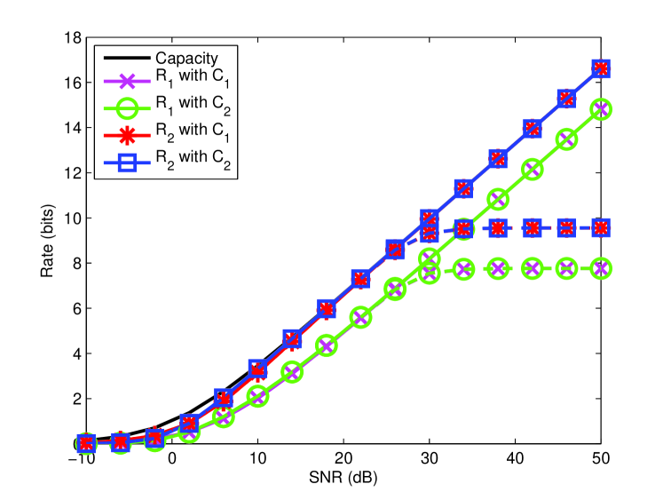
Figure 2: Numerical results. $R_{1}$: The rate obtained by considering carry over as noise. $R_{2}$: The rate obtained by decoding carry overs at each level. $C_{1}$: Choosing $p_{l}$ from the binary expansion of the exponential distribution with mean $E_{X}+E_{N}$. To satisfy the power constraint, only a fraction of the channel uses (i.e., $\frac{E_{X}}{E_{X}+E_{N}}$ of the time) is utilized. $C_{2}$: Choosing $p_{l}$ from the binary expansion of the exponential distribution with mean $E_{X}$. Solid and dotted curves correspond to coding over $41$ and $21$ number of levels, respectively.

V Discussion

We note the followings.

• Expansion coding allows the construction of good channel codes for discrete-time continuous channels using good discrete memoryless channel codes. For instance, one can utilize binary expansion together with polar codes. The underlying code is $q$-ary polar code, as we need to implement Gallager’s method in constructing the input distribution $p(x)=\textrm{Ber}(p_{l})$ for coding over level $l$. (See, e.g., [5, 7] for details.) In addition, expansion modulation can be implemented over a $q$-ary expansion of the channel, and any good code for the resulting modulo $q$-sum channel can be used.

• Avestimehr et al. [8] have introduced the deterministic approximation approach for point-to-point and multi-user channels. The basic idea is to construct an approximate channel for which the transmitted signals are assumed to be noiseless above the noise level. Using this high SNR approximation, one only needs to deal with the interference seen at a particular receiver (in a networked model). Our expansion coding scheme can be seen as a generalization of these deterministic approaches. Here, the (effective) noise in the channel is carefully calculated and the system takes advantage of coding over the noisy levels at any SNR. This generalized channel approximation approach can be useful in reducing the large gaps reported in the previous works.

• Although our discussion is limited to the AEN channel, where the proposed scheme outperforms the previously proposed modulation schemes and performs arbitrarily close to the capacity of the AEN channel, the expansion coding refers to a more general framework and is not limited to such channels. Towards this end, our ongoing efforts are focused on utilizing the proposed scheme for AEN multiple-user channels, and for their AWGN counterparts.

Appendix A Proof of Lemma 4

Recall that, in our construction, $q_{l}$ is the probability that Bernoulli random variable takes value 1 at level $l$. Thus,

$$H(q_{l}) =-q_{l}\log q_{l}-(1-q_{l})\log(1-q_{l})$$

$$=-\frac{1}{1+e^{2^{l}}}\log\frac{1}{1+e^{2^{l}}}-\frac{e^{2^{l}}}{1+e^{2^{l}}}\log\frac{e^{2^{l}}}{1+e^{2^{l}}}.$$

When $l\leq 0$, we obtain a lower bound as

$$H(q_{l}) =\log\left(1+e^{2^{l}}\right)-\frac{e^{2^{l}}}{1+e^{2^{l}}}\log e\cdot 2^{l}$$

$$>\log(1+1)-\log e\cdot 2^{l}$$

$$=1-\log e\cdot 2^{l}.$$

On the other hand, when $l\geq 0$, by using the facts that $\log(1+x)<\log e\cdot x$ for any $0<x<1$, and $e^{x}>1+x+x^{2}/2$ for any $x>0$, we have

$$H(q_{l}) =\frac{1}{1+e^{2^{l}}}\log\left(1+e^{2^{l}}\right)+\frac{e^{2^{l}}}{1+e^{2^{l}}}\log\left(1+e^{-2^{l}}\right)$$

$$<\frac{1}{1+e^{2^{l}}}\log\left(2e^{2^{l}}\right)+\log\left(1+e^{-2^{l}}\right)$$

$$<\frac{1+2^{l}\log e}{1+e^{2^{l}}}+e^{-2^{l}}\log e$$

$$<\frac{1+2^{l}\log e}{1+1+2^{l}+2^{2l}/2}+\frac{1}{1+2^{l}}\log e$$

$$<2^{-l}2\log e+2^{-l}\log e$$

$$=2^{-l}3\log e.$$

References

• [1] S. Verdú, “The exponential distribution in information theory,” Problems of Information Transmission, vol. 32, no. 1, pp. 86–95, Jan.-Mar. 1996.
• [2] A. Martinez, “Communication by energy modulation: The additive exponential noise channel,” IEEE Trans. on Inf. Theory, vol. 57, no. 6, pp. 3333–3351, Jun. 2011.
• [3] S. Y. Le Goff, “Capacity-approaching signal constellations for the additive exponential noise channel,” CoRR, vol. abs/1111.6414, 2011.
• [4] G. Marsaglia, “Random variables with independent binary digits,” Ann. Math. Statist., vol. 42, no. 6, pp. 1922–1929, 1971.
• [5] E. Arıkan, “Channel polarization: A Method for constructing capacity-achieving codes for symmetric binary-input memoryless channels,” IEEE Trans. on Inf. Theory, vol. 55, no. 7, pp. 3051–3073, Jul. 2009.
• [6] R. G. Gallager, Information Theory and Reliable Communication.   John Wiley & Sons, Inc., 1968.
• [7] E. Sasoglu, E. Arıkan, and E. Telatar, “Polarization for arbitrary discrete memoryless channels,” in Proc. 2009 IEEE Information Theory Workshop (ITW 2009), Taormina, Sicily, Italy, Oct. 2009.
• [8] A. Avestimehr, S. Diggavi, and D. Tse, “Wireless Network Information Flow: A Deterministic Approach,” IEEE Trans. Inf. Theory, vol. 57, no. 4, pp. 1872–1905, Apr. 2011.