Abstract

We study the nonconserved phase ordering dynamics of the $d=2,3$ random field Ising model, quenched to below the critical temperature. Motivated by the puzzling results of previous work in two and three dimensions, reporting a crossover from power-law to logarithmic growth, together with superuniversal behavior of the correlation function, we have undertaken a careful investigation of both the domain growth law and the autocorrelation function. Our main results are as follows: We confirm the crossover to asymptotic logarithmic behavior in the growth law, but, at variance with previous findings, the exponent in the preasymptotic power law is disorder-dependent, rather than being the one of the pure system. Furthermore, we find that the autocorrelation function does not display superuniversal behavior. This restores consistency with previous results for the $d=1$ system, and fits nicely into the unifying scaling scheme we have recently proposed in the study of the random bond Ising model.

1 Introduction

Much recent interest in statistical physics has focused on understanding out-of-equilibrium phenomena. In this context, of paramount importance are slow relaxation phenomena, which primarily occur in glassy systems. An important hallmark of slow relaxation is the lack of time-translation-invariance, manifested through aging behavior. A similar phenomenology is also observed in systems without disorder, e.g., ferromagnets quenched below the critical point. The behavior of these systems is well understood in terms of the domain growth mechanism of slow relaxation [1, 2].

The key feature of domain growth, or coarsening, is the unbounded growth of the domain size, which entails scaling due to the existence of a dominant length scale, and aging as a manifestation of scaling in multiple-time observables. The simplicity of this structure is very attractive and is expected to be valid beyond the realm of disorder-free phase-separating systems, establishing domain growth as a paradigm of slow relaxation. However, as is well known, the applicability of domain growth concepts to hard problems (such as spin glasses or structural glasses) still remains a debated issue [3]. Therefore, it is of considerable interest to study the role of disorder in systems where its presence does not compete with phase ordering [4].

A class of systems of this type are disordered ferromagnets, where disorder coexists with the low-temperature ferromagnetic order. There are different ways to introduce disorder in a ferromagnet without inducing frustration. This can be achieved through bond or site dilution, by randomizing the exchange interaction strength while keeping it ferromagnetic, or by introducing a random external field. These disordered systems have been an active area of research for quite some time now. The unifying theme of investigation has been disorder-induced changes in the properties of the underlying pure systems, with primary interest in the growth law, in the equal-time correlation function and, more recently, in the two-time autocorrelation function and the related response function [5, 6, 7, 8, 9]. However, despite the many experimental and theoretical studies [4], a number of issues are still open. Among these, of primary importance are (i) the nature of the asymptotic growth law (power-law vs. logarithmic) and (ii) the existence of superuniversal behavior of the correlation and response functions. This is the idea that scaling functions are robust with respect to disorder, which is expected not to change the low temperature properties of the system [10]. The lack of a general framework to understand this complex phenomenology has proven a major obstacle to development. Recently, in the context of the random bond Ising model (RBIM) [9], we have shown that the renormalization group (RG) picture of crossover phenomena may well serve the purpose.

In this paper, we extend the RG conceptual framework to the ordering dynamics of the random field Ising model (RFIM) [11]. In this system, the deep asymptotic regime turns out to be numerically accessible, allowing us to make precise statements regarding the growth law and the superuniversality (SU) issue (see subsection 2.1). Our principal findings are (a) the existence of a crossover from power law domain growth (with a disorder-dependent exponent) to logarithmic growth, and (b) the absence of SU. Both results fit nicely into an RG picture where disorder acts as a relevant perturbation with respect to the pure fixed point. This confirms the robustness and the general applicability of the approach proposed in Ref. [9].

This paper is organized as follows. In Sec. 2, we provide an overview of domain growth laws and of our scaling framework for phase ordering dynamics in disordered systems. In Sec. 3, we present detailed numerical results for ordering in the $d=2$ RFIM. These results are interpreted using the scaling framework of Sec. 2. Sec. 4 is devoted to the presentation of numerical results in the $d=3$ case. Finally, in Sec. 5, we conclude this paper with a summary and discussion.

2 Domain Growth Laws in Disordered Systems

Dynamical scaling is the most important characteristic of phase ordering systems [1, 2]. Let us summarise the concept in the simplest case of pure systems. As time increases, the typical domain size $L(t)$ grows and becomes the dominant length in the problem. Then, all other lengths can be rescaled with respect to $L(t)$. For instance, the two-time order-parameter correlation function $C(r,t,t_{w})$, with $t_{w}\leq t$, scales as [12, 13]

$$C(r,t,t_{w})=G(r/L,L/L_{w})$$ (1)

where $L$ and $L_{w}$ stand for $L(t)$ and $L(t_{w})$, respectively. This contains, as a special case, the usual scaling of the equal-time ($t=t_{w}$) correlation function $C(r,t)=G_{1}(r/L)$. Further, for $r=0$, we have the aging form of the autocorrelation function $C(t,t_{w})=G_{2}(L/L_{w})$. The validity of scaling is, by now, a well-established fact. A complete picture of an ordering problem requires the understanding of the growth law (i.e. how $L(t)$ depends on $t$) and of the scaling function $G(x,y)$.

A systematic study of the growth law has been undertaken by Lai et al. (LMV) [14, 15], who identified four different universality classes of growth kinetics. LMV considered the role of several factors in the ordering dynamics, e.g., temperature, conservation laws, dimensionality, order parameter symmetry, lattice structure and disorder. An important distinction is made between systems that do not freeze (i.e., without free-energy barriers) and those that do freeze (i.e., with barriers) when the quench is made to $T=0$. To the first category belong pure systems with non-conserved dynamics, whose growth follows the power law $L(t)=Dt^{1/z}$, where $z=2$. LMV designate these as Class 1 systems. To the second category belong systems whose growth requires thermal activation. This includes pure systems with conserved order parameter and systems (both conserved and non-conserved) with quenched disorder. This category is further subdivided into three classes. In Class 2 systems the freezing involves only local defects, with activation energy $E_{B}$ independent of the domain size. In this case, growth is still power law: $L(t)=Dt^{1/z}$ with $z=2$ and 3 for the non-conserved and conserved cases, respectively. Furthermore, the prefactor $D$ has a strong temperature dependence, $D\sim e^{-E_{B}/(zT)}$. Finally, in Class 3 and Class 4 systems, the freezing involves a collective behavior which depends on the domain size $L$. If the corresponding activation energy scales with $L$ like $E_{B}(L)\sim\epsilon L^{\varphi}$, where $\epsilon$ measures the disorder strength, the asymptotic growth law is logarithmic

$$L(t)\sim(T/\epsilon)^{1/\varphi}\left[\ln(t/\tau)\right]^{1/\varphi}$$ (2)

with $\tau\sim T/(\varphi\epsilon)$. For Class 3 systems, we have $\varphi=1$, and for Class 4 systems, we have $\varphi\neq 1$.

Ferromagnets (with or without disorder) offer examples of the classes listed above. For simplicity, let us consider systems with non-conserved order parameter. The pure ferromagnetic Ising model with Glauber kinetics is a well-known Class 1 system [1]. The $d=1$ ferromagnetic RBIM [7] is an example of a Class 2 system. The $d=1$ RFIM [16] belongs to Class 4, with $\varphi=1/2$. The RFIM in higher dimensions, $d=2$ [17, 18] and $d=3$ [19, 20], shows logarithmic growth, although it is not easy to unambiguously establish the value of $\varphi$. Recently, we have presented evidence [9] for logarithmic growth in the $d=2$ RBIM, but have not established whether it is a Class 3 or Class 4 system. This is a particularly interesting system, because its growth law was previously [21] believed to be power law with a disorder-dependent exponent. If so, this would have shown the existence of a new universality class, say Class 5, in addition to the four listed by LMV. We should stress that a huge numerical effort is involved in accessing the logarithmic growth regime of the $d=2$ RBIM, and our understanding of this system remains incomplete.

In Ref. [9], we have proposed to unify this wide variety of behaviors for disordered domain growth into a scaling framework for the growth law itself. In all the cases we consider in this paper, disorder ($h_{0}$) and temperature ($T$) enter through their ratio $h_{0}/T$ (see Sec. 3.1 below). This will be denoted by $\epsilon$ and, for short, will be termed as disorder. Let us begin with the straightforward crossover set-up, where the growth law is assumed to scale as

$$L(t,\epsilon)=t^{1/z}F(\epsilon/t^{\phi}),$$ (3)

$z=2$ is the growth exponent for non-conserved dynamics in a pure ferromagnet and $\phi$ is the crossover exponent. With the additional assumption that the scaling function behaves as

$$F(x)\sim\left\{\begin{array}[]{ll}$const.$,\;\;$for$\;\;x\rightarrow 0,\\ x^{1/(\phi z)}\ell(x^{-1/\phi}),\;\;$for$\;\;x\rightarrow\infty,\end{array}\right.$$ (4)

where $x=\epsilon/t^{\phi}$, Eq. (3) describes the crossover from the power law $L(t)\sim t^{1/z}$ to the asymptotic form $L(t)\sim\ell\left(t/\epsilon^{1/\phi}\right)$, if $\phi<0$, and vice-versa if $\phi>0$. Alternatively, disorder is asymptotically relevant when $\phi<0$, and irrelevant when $\phi>0$. The key quantity in the analysis of crossover is the effective growth exponent

$${1\over z_{\rm eff}(t,\epsilon)}={\partial\ln L(t,\epsilon)\over\partial\ln t}={1\over z}-\phi{\partial\ln F(x)\over\partial\ln x},$$ (5)

which depends on $t$ and $\epsilon$ through $x$.

In the following discussion, it will be useful to use the above relations in the inverted form:

$$t=L^{z}g(L/\lambda),$$ (6)

where

$$\lambda=\epsilon^{1/(\phi z)}$$ (7)

is a length scale associated with disorder. The scaling functions appearing in Eqs. (3) and (6) are related by

$$g(y)=F^{-z}(x)$$ (8)

and $y=L/\lambda$ is related to $x$ by

$$y=x^{-1/(\phi z)}F(x).$$ (9)

Then, from Eq. (4) and $\phi<0$, it follows that

$$g(y)\sim\left\{\begin{array}[]{ll}$const.$,\;\;$for$\;\;y\ll 1,\\ y^{-z}\ell^{-1}(y),\;\;$for$\;\;y\gg 1,\end{array}\right.$$ (10)

where $\ell^{-1}$ stands for the inverse function of $\ell$. The opposite behavior holds for $\phi>0$

$$g(y)\sim\left\{\begin{array}[]{ll}y^{-z}\ell^{-1}(y),\;\;$for$\;\;y\ll 1,\\ $const.$,\;\;$for$\;\;y\gg 1.\end{array}\right.$$ (11)

Finally, the effective exponent as a function of $y$ is obtained from Eq. (6)

$$z_{\rm eff}(y)=z+{\partial\ln g(y)\over\partial\ln y}.$$ (12)

Therefore, for $\phi<0$ (disorder relevant), Eq. (10) yields

$$z_{\rm eff}(y)=\left\{\begin{array}[]{ll}z,\;\;$for$\;\;y\ll 1,\\ \partial\ln\ell^{-1}(y)/\partial\ln y,\;\;$for$\;\;y\gg 1,\end{array}\right.$$ (13)

and for $\phi>0$ (disorder irrelevant), we obtain from Eq. (11)

$$z_{\rm eff}(y)=\left\{\begin{array}[]{ll}\partial\ln\ell^{-1}(y)/\partial\ln y,\;\;$for$\;\;y\ll 1,\\ z,\;\;$for$\;\;y\gg 1.\end{array}\right.$$ (14)

2.1 Superuniversality

One would expect that the above crossover scenario, which is well established for the growth law, would extend also to the other observables. However, this expectation is in conflict with the SU statement that all disorder dependence in observables other than the growth law can be eliminated by reparametrization of time through $L(t,\epsilon)$ [10]. Thus, according to SU, for the autocorrelation function one should have

$$C(t,t_{w},\epsilon)=G_{2}(L(t_{w},\epsilon)/L(t_{w},\epsilon))$$ (15)

where $G_{2}$ is the scaling function of the pure case. The validity of SU is controversial, since the $d=1$ results [7, 16] clearly demonstrate the absence of SU, while from the study of the correlation function for $d\geq 2$, there is evidence both in favour [19, 20, 21, 22] and against [9] SU validity. Recently, the validity of SU has been extended to the geometrical properties of domain structures [23].

In the next sections we present comprehensive numerical results from large scale simulations of ordering dynamics in the RFIM in $d=2,3$. We will analyze numerical results within the above scaling framework, producing evidence against SU validity.

3 Numerical Results for $d=2$

3.1 Simulation Details

We consider an RFIM on a two-dimensional square lattice, with the Hamiltonian

$$H=-J\sum_{\langle ij\rangle}\sigma_{i}\sigma_{j}-\sum_{i=1}^{N}h_{i}\sigma_{i},~{}~{}~{}~{}~{}~{}~{}\sigma=\pm 1,$$ (16)

where $\langle ij\rangle$ denotes a nearest-neighbour pair, and $J>0$ is the ferromagnetic exchange coupling. The random field $h_{i}=\pm h_{0}$ is an uncorrelated quenched variable with a bimodal distribution

$$P(h_{i})=\frac{1}{2}\left[\delta(h_{i}-h_{0})+\delta(h_{i}+h_{0})\right].$$ (17)

The system evolves according to the Glauber kinetics, which models nonconserved dynamics [2], with spin flip transition rates given by

$$w(\sigma_{i}\rightarrow-\sigma_{i})=\frac{1}{2}\left(1-\sigma_{i}\tanh\left((H_{i}^{W}+h_{i})/T\right)\right)$$ (18)

where $H_{i}^{W}$ is the local Weiss field. All results in this paper correspond to the limit $T\rightarrow 0$ ($J/T\rightarrow\infty$), while keeping the ratio $\epsilon=h_{0}/T$ finite. In this limit the system undergoes phase ordering in any dimension, down to $d=1$ [16]. The transition rates take the form

$$w(\sigma_{i}\rightarrow-\sigma_{i})=\left\{\begin{array}[]{ll}1\;\;$for$\;\;H_{i}^{W}\sigma_{i}<0,\\ 0\;\;$for$\;\;H_{i}^{W}\sigma_{i}>0,\\ \frac{1}{2}\left(1-sign(\sigma_{i}h_{i})\tanh(\epsilon)\right)\;\;$for$\;\;H_{i}^{W}=0\end{array}\right.$$ (19)

which shows that disorder affects the evolution through the ratio $\epsilon=h_{0}/T$, as anticipated in Sec. 2. Moreover, Eq. (19) allows for an accelerated updating rule, with a considerable increase in the speed of computation [24], by restricting updates to the sites with $H_{i}^{W}\sigma_{i}\leq 0$, whose number decreases in time as $1/L(t)$. The gain in the speed of computation becomes more important the longer the simulation.

All statistical quantities presented here have been obtained as an average over $N_{\rm run}=10$ independent runs. For each run, the system has different initial condition and random field configuration. We have considered the values of disorder amplitude $\epsilon=0,0.25,0.5,1,1.5,2,2.5$ and we have carefully checked that no finite size effects are present up to the final simulation time when $N=8000^{2}$ spins. In the pure case, since coarsening is more rapid, we have taken $N=12000^{2}$.

Numerical results for the growth law and the autocorrelation function are presented in the following subsections.

3.2 Growth Law

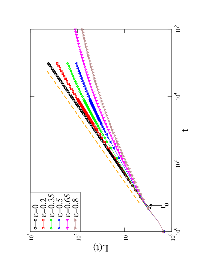
We have obtained the characteristic $L(t)$ from the inverse density of defects. This is measured by dividing the number of sites with at least one oppositely-aligned neighbor by the total number of sites. The plot of $L(t,\epsilon)$ vs. $t$, in Fig. 1, shows the existence of at least two time-regimes, separated by a microscopic time $t_{0}$ of order 1. In the early-time regime (for $t<t_{0}$), there is no dependence on disorder and growth is fast. This is the regime where the defects seeded by the random initial condition execute rapid motion toward the nearby local minima. For $\epsilon>0$ and $t>t_{0}$, there is a strong dependence on disorder producing slower growth and deviation from the power law behavior of the pure case (top cicles line in Fig. 1).

Figure 1: (Color online) Growth law in $d=2$. The dashed line is the $t^{1/2}$ growth law.

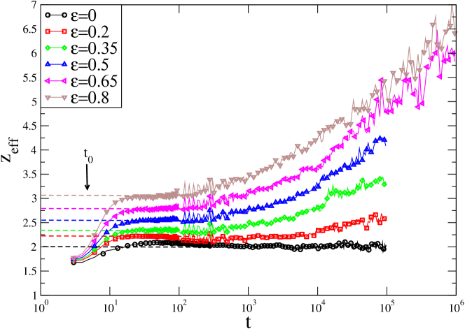
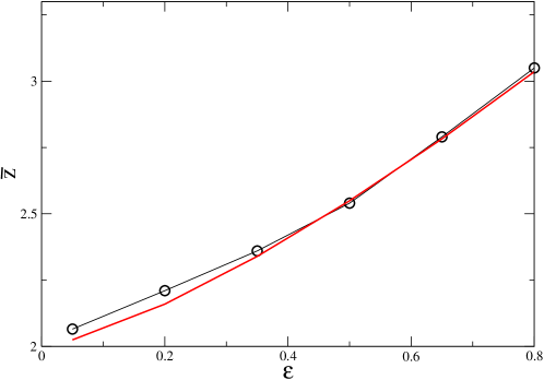
In Fig. 2, we show the time-dependence of the effective exponent $z_{\rm eff}(t,\epsilon)$, defined by Eq. (5). For $t>t_{0}$, this plot shows the existence of an intermediate power-law regime, characterized by a plateau where $z_{\rm eff}$ is approximately constant. This is followed by the late regime where $z_{\rm eff}$ is clearly time-dependent. The disorder dependent values of $z_{\rm eff}$ on the plateaus, denoted by $\overline{z}$, are listed in Table 1 and plotted in Fig. 3. We encountered a similar crossover in our study of the $d=2$ RBIM [9], i.e., a preasymptotic power law regime with a disorder dependent exponent, followed by an asymptotic regime where the growth law deviates from a power law.

Figure 2: (Color online) Effective exponent $z_{\rm eff}$ vs. $t$ in $d=2$. The horizontal dashed lines indicate $\overline{z}$, the plateau values of $z_{\rm eff}$.

Figure 3: (Color online) $\overline{z}$ (taken from Fig. 2) vs. $\epsilon$. The red line is the best fit $\overline{z}=2.0+1.4\epsilon^{1.35}$.

$\epsilon$	$\overline{z}$
$0$	$2$
$0.2$	$2.20$
$0.35$	$2.31$
$0.5$	$2.52$
$0.65$	$2.77$
$0.8$	$3.05$

Table 1: Plateau exponent $\overline{z}$ for various disorder strengths.

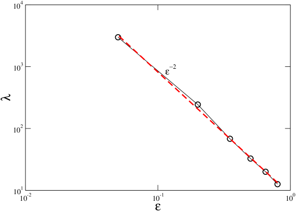
The appearance of a disorder dependent exponent $\overline{z}$ in the intermediate regime suggests to upgrade the crossover picture, presented in Sec. 2, by replacing the pure growth exponent $z$ by $\overline{z}$ in all the scaling formulae. Then, from Eq. (12) it follows that $z_{\rm eff}-\overline{z}$ ought to depend only on $y=L/\lambda$. Indeed, as Fig. 4 shows, it is possible to determine numerically the quantity $\lambda$ such that the plots of $(z_{\rm eff}-\overline{z})$ vs. $L/\lambda$, for different disorder values, collapse on a single master curve. The $\epsilon$-dependence of $\lambda$ is displayed in Fig. 5 and is well fitted by

$$\lambda\sim\epsilon^{-2}.$$ (20)

Comparing this with Eq. (7), the negative exponent implies $\phi<0$ and, therefore, that disorder acts like a relevant scaling field. This is also confirmed by the behavior of $z_{\rm eff}(y)$ in Fig. 4, which is consistent with Eq. (13) but not with Eq. (14).

Figure 4: (Color online) Subtracted effective exponent $(z_{\rm eff}-\overline{z})$ vs. $L/\lambda$. The dashed line is the best fit $z_{\rm eff}-\overline{z}=0.0055(L/\lambda)^{1.5}$.

Figure 5: (Color online) Plot of $\lambda$ vs. $\epsilon$.

Fitting the data of Fig. 4 to the power law $z_{\rm eff}-\overline{z}=by^{\varphi}$, we find $b\simeq 0.0055$ and $\varphi\simeq 1.5$. Hence, from the definition of $z_{\rm eff}$ in Eq. (5) follows

$${\partial\ln t\over\partial L}=\overline{z}+by^{\varphi}$$ (21)

which, after integrating with respect to $L$, yields

$$t=K(\epsilon)L^{\overline{z}}g(L/\lambda)$$ (22)

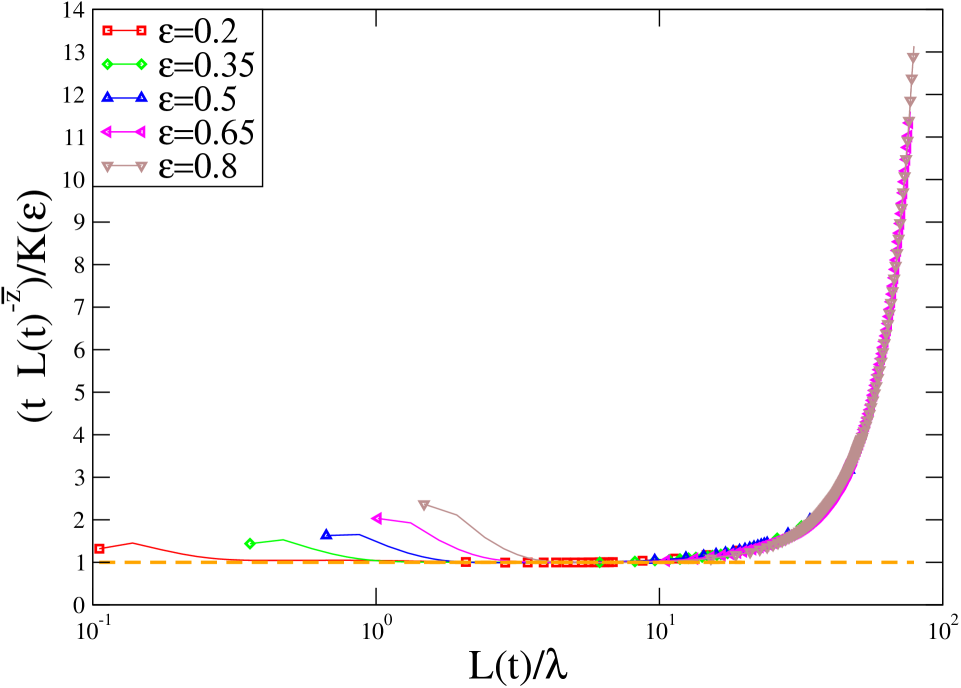
where $K(\epsilon)$ is an $\epsilon$-dependent prefactor. Indeed, replotting in Fig. 6 the data of Fig. 1, as $tL^{-\overline{z}}/K(\epsilon)$ vs. $y$, an excellent data collapse on the master curve

$$g(y)\sim\exp\left(\frac{b}{\varphi}y^{\varphi}\right)$$ (23)

is obtained, with the values of $K(\epsilon)$ listed in Table 2.

$\epsilon$	$K$
$0.5$	$0.39$
$1.0$	$0.13$
$1.5$	$0.039$
$2.0$	$0.015$

Table 2: Prefactor $K(\epsilon)$ for various disorder strengths.

The plot of the scaling function $g(y)$ illustrates quite effectively (i) the existence of the crossover, and (ii) that our numerical data reach deep into the asymptotic regime. The flat part of the curve, where $g(y)$ lies on the horizontal dashed line at $g(y)=1$, corresponds to the preasymptotic power-law regime [cf. Eq. (10)]. The sharp and fast increase of $g(y)$, for large $y$, corresponds to the crossover to the asymptotic growth law

$${L\over\lambda}\simeq\left[{\varphi\over b}\ln\left(t/\lambda^{\overline{z}}\right)\right]^{1/\varphi}$$ (24)

which corresponds to the Class 4 form of Eq. (2).

Summarising, our main findings for the growth law, in the $d=2$, case are as follows:

1. Disorder is a relevant perturbation with respect to pure-like behavior.

2. The corresponding growth law shows a clear crossover from power-law to logarithmic behavior:

   $$L(t,\epsilon)\sim\left\{\begin{array}[]{ll}t^{1/\overline{z}},\;\;$if$\;\;L\ll L_{\rm cr},\\ (\ln t)^{1/\varphi},\;\;$if$\;\;L\gg L_{\rm cr}.\end{array}\right.$$ (25)

   This differs from previously found results, since the preasymptotic power law is not pure-like, due to the $\epsilon$-dependence of the exponent $\overline{z}$. This feature, also observed in the $d=2$ RBIM [9], means that disorder although globally relevant acts like a marginal operator in the neighborhood of the pure fixed point [25].

Finally, we remark on the considerable numerical advanyage in using the effective exponent as a probe for the crossover. In fact, while the switch from preasymptotic to asymptotic behaviors in $z_{\rm eff}$ takes place at about $L_{\rm cr}\simeq\lambda$, from Eqs. (22) and (23), it follows that the condition $by^{\varphi}/\varphi=1$ puts the crossover, when looking at the domain size, at the much greater value $L_{\rm cr}\simeq 50\lambda$, as it is evident from Fig. 6.

Figure 6: (Color online) Plot of $tL^{-\overline{z}}/K(\epsilon)$ vs. $L/\lambda$ with various disorder values. The master curve obeys the exponential form of Eq. (23).

3.3 Autocorrelation Function and SU Violation

The results presented above show that disorder affects the growth law as an asymptotically relevant parameter. Therefore, one would expect this to apply also to other observables. However, as explained in Sec. 2.1, such an expectation would be in conflict with claims of SU validity.

In this section, we study the autocorrelation function, defined by

$$C(t,t_{w},\epsilon)=\langle\sigma_{i}(t)\sigma_{i}(t_{w})\rangle$$ (26)

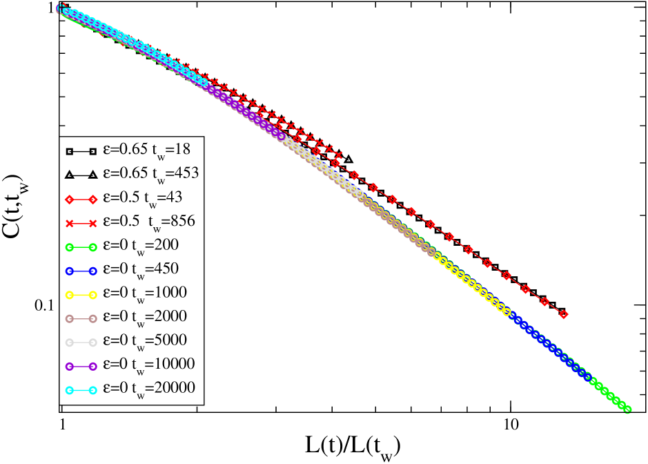
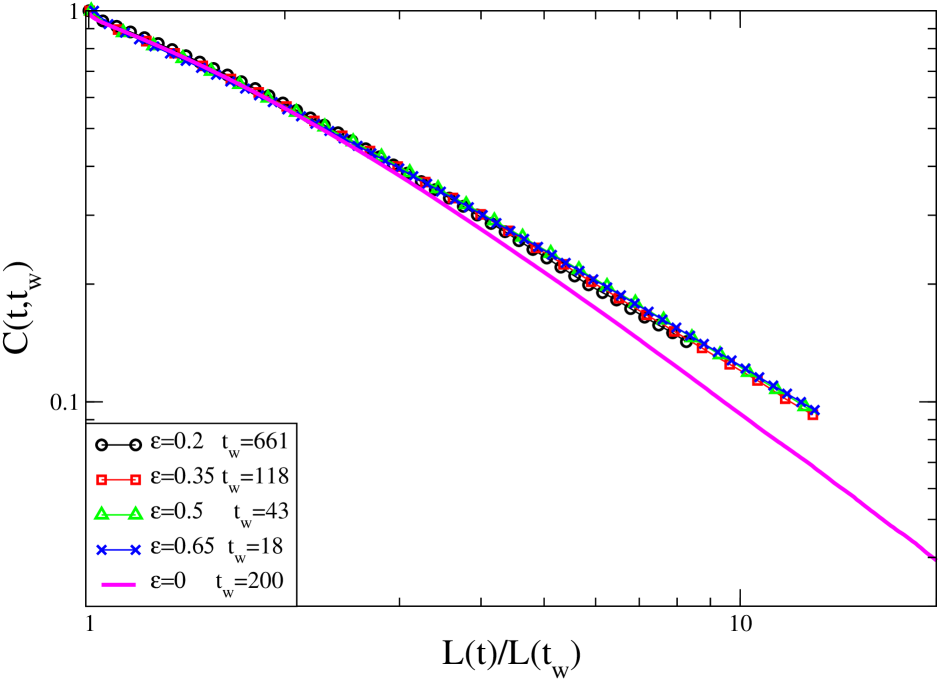
which is independent of $i$, due to space-translation invariance. In Fig. 7 $C(t,t_{w},\epsilon)$ has been plotted against $L/L_{w}$, for $\epsilon=0,0.5,0.65$ and with different values of $t_{w}$, chosen in such a way that the ratio $v=L_{w}/\lambda$ takes the three different values $v=0,0.25,0.85$. If SU were valid all the curves, irrespective of the value of $\epsilon$, should collapse on the $\epsilon=0$, or $v=0$, master curve. Instead, there is an evident $\epsilon$-dependence which excludes SU validity. In addition, curves with the same value of $v$ do collapse, showing that the autocorrelation function obeys the extended aging form

$$C(t,t_{w},\epsilon)=h\left({L\over L_{w}},{\lambda\over L_{w}}\right).$$ (27)

The pure master curve, with $v=0$, lies below the two corresponding to $v=0.25$ and $v=0.85$. Figure 8 displays a similar plot, with $v=0$ and $v=0.25$. The latter value is obtained by combining the four different values of disorder $\epsilon=0.2,0.35,0.5,0.65$ with appropriately chosen $t_{w}$-values. Again, there are two distinct master curves for different $v$-values.

Figure 7: (Color online) Autocorrelation function in $d=2$, for disorder values and waiting times $t_{w}$ chosen so that $v=L_{w}/\lambda$ takes the three values $v=0,0.25,0.85$ corresponding, from bottom to top, to the three different master curves.

Figure 8: (Color online) Analogous to Fig. 7, with $v=0$ (lower master curve) and $v=0.25$ (upper master curve).

The reported SU violation is in agreement with the behavior of the autocorrelation function in the $d=1$ RFIM [16].

4 Numerical Results for $d=3$

As mentioned above, in previous studies of the $d=3$ RFIM [19, 20] SU has been found to hold. Here, instead, we present new results for this system, which produce evidence for the same pattern of SU violation observed in the $d=2$ case.

Simulations were made on a system with $N=300^{3}$ spins on a cubic lattice, evolving with the transition rates (19) and averaging over $N_{\rm run}=20$ runs, each with different initial condition and random field configuration. We have considered the three disorder values $\epsilon=0.5,1,2$. Although the quality of the data does not allow for an analysis of high precision as in the $d=2$ case discussed above, nonetheless the main features, including the lack of SU validity, do emerge quite clearly.

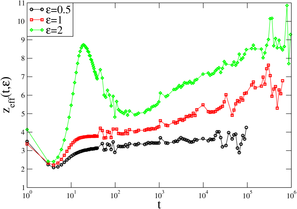
Let us begin with the growth law. The $L(t)$ data have been plotted in Fig. 9. The qualitative behaviour is the same as in Fig. 1, namely, as disorder increases, growth slows down. The corresponding effective exponent $z_{\rm eff}$ is displayed in Fig. 10. For the smaller values, $\epsilon=0.5$ and $\epsilon=1$, the overall behaviour is qualitatively similar to that of Fig. 2, showing a crossover from power law (with disorder dependent exponent) to logarithmic behavior, as in Eq. (25). The data for the highest disorder value $\epsilon=2$, instead, display a novel behaviour. The preasymptotic power law regime disappears and is replaced by a pronounced peak in the effective exponent, which reveals strong pinning of the interfaces. Therefore, the nature of the crossover is qualitatively different for weak and for strong disorder. The detailed investigation of this novel feature is delayed to a future publication.

Figure 9: (Color online) Growth law in $d=3$ for different disorder values.

Figure 10: (Color online) Effective exponent $z_{\rm eff}(t,\epsilon)$ in $d=3$.

The data for the autocorrelation function are displayed in Fig. 11. As stated above, the quality of the data is not sufficient to carry out a precise scaling analysis as in Sec. 3. In particular, it is not possible to extract the characteristic length $\lambda$ reliably and to organise the plot with a choice of $t_{w}$ values aimed to keep constant the ratio $L_{w}/\lambda$. However, the evident $\epsilon$-dependence in Fig. 11 is quite sufficient to exclude SU validity.

As a final remark, it should be noted that with the algorithm illustrated in Sec. 3.1 we consider a quench to $T=0$, while in Refs. [19, 20] quenches to $T>0$ were considered. Therefore, it remains an open question, to be investigated, whether the discrepancy between ours and previous results may be related to the role of the final temperature.

Figure 11: (Color online) Autocorrelation function in $d=3$ for different $\epsilon$ and $t_{w}$ values.

5 Summary and Discussion

Let us conclude this paper with a summary and discussion of our results. We have recently initiated a large-scale simulation study of nonconserved domain growth in disordered systems. Our study was motivated by some ambiguities existing in the available literature:
(a) The precise nature of the asymptotic growth law in the standard models (RBIM, RFIM, etc.) was unclear.
(b) Quantities like the equal-time correlation function (or its Fourier transform, the structure factor) showed SU, i.e., the scaling functions were independent of disorder. It was not clear to us why the crossover in the domain growth law was not accompanied by a corresponding crossover in the correlation function.
(c) There were very few studies of two-time quantities like the autocorrelation function and the response function.

With this background, we investigated two-time quantities in the $d=1,2$ RBIM [7, 9] and, with the present paper, we have extended the investigation to the $d=2,3$ RFIM with Glauber spin-flip kinetics. Our results can be summarized as follows:
(i) First, we have formulated a general scaling framework for the study of disordered domain growth. The framework is based on the RG concept of asymptotically relevant parameter, and proved very convenient for interpreting our earlier RBIM results [9]. In this paper, we have used this framework to successfully understand crossovers in the RFIM.
(ii) Second, we find that there is a crossover in the domain growth law from a preasymptotic regime showing power law growth with a disorder dependent exponent [$L(t)\sim t^{1/\overline{z}(\epsilon)}$] to an asymptotic regime with logarithmic growth [$L(t)\sim(\ln t)^{1/\varphi}$ with $\varphi\simeq 1.5$]. Following the analysis of Ref. [21], this can be related to an underlying crossover from logarithmic dependence of the free energy barriers on the domain size to power law dependence. The mechanism producing the power law dependence is particularly clear in $d=1$, where the interface motion can be mapped into the random walk in a random potential of the Sinai type [16, 27].
(iii) Third, and perhaps most important, we find that the autocorrelation function does not obey SU. The scaling function shows a crossover corresponding to the crossover in the growth law.

In the light of the above results, what is the path ahead? We are currently investigating other disordered systems to confirm whether the domain growth scenario is consistent with the scaling picture developed here. It is also relevant to re-examine earlier results demonstrating SU for the equal-time correlation function. It is possible that the equal-time correlation function has a delayed crossover, and may violate SU in larger and longer simulations. Alternatively, it could be that the equal-time correlation function is a relatively crude and feature-less characteristic of the morphology. It may be worthwhile to study more sophisticated measures of the morphology [26], which could show differences between pure and disordered phase ordering systems. Our studies demonstrate that there remain many unanswered questions in this area. We hope that our work will motivate fresh interest in these problems.

References

- [1] A.J. Bray, Adv. Phys. 43, 357 (1994).
- [2] S. Puri, in Kinetics of Phase Transitions, edited by S. Puri and V. Wadhawan, CRC Press, Boca Raton (2009), p. 1.
- [3] For reviews, see J.P.Bouchaud, L.F.Cugliandolo, J.Kurchan and M.Mezard, Out of equilibrium dynamics in spin-glasses and other glassy systems, in Spin Glasses and Random Fields, edited by A.P.Young, World Scientific, Singapore (1997); L.F.Cugliandolo, Dynamics of glassy systems, in Slow Relaxation and Non-Equilibrium Dynamics in Condensed Matter, edited by J.L.Barrat, J.Dalibard, J.Kurchan and M.V.Feigel’man, Springer-Verlag, Heidelberg (2002).
- [4] S. Puri, Phase Transitions 77, 469 (2004).
- [5] M. Henkel and M. Pleimling, Europhys. Lett. 76, 561 (2006).
- [6] M. Henkel and M. Pleimling, Phys. Rev. B 78, 224419 (2008).
- [7] E. Lippiello, A. Mukherjee, S. Puri and M. Zannetti, Europhys. Lett. 90, 46006 (2010).
- [8] H. Park and M. Pleimling, Phys. Rev. B 82, 144406 (2010).
- [9] F. Corberi, E. Lippiello, A. Mukherjee, S. Puri and M. Zannetti, J. Stat. Mech.: Theory and Experiment P03016 (2011).
- [10] L.F. Cugliandolo, Physica A 389, 4360 (2010). For an explanation of the superuniversality concept see Sec. 5.2 and references quoted therein.
- [11] T.Nattermann, Theory of the random field Ising model, in Spin Glasses and Random Fields, A.P.Young Ed., World Scientific, Singapore (1997).
- [12] H. Furukawa, J. Phys. Soc. Japan 58 216 (1989); Phys. Rev. B 40, 2341 (1989).
- [13] M. Zannetti, in Kinetics of Phase Transitions, edited by S. Puri and V. Wadhawan, CRC Press, Boca Raton (2009), p. 153.
- [14] Z.W. Lai, G.F. Mazenko and O.T. Valls, Phys. Rev. B 37, 9481 (1988).
- [15] K. Tafa, S. Puri and D. Kumar, Phys. Rev. E 63, 046115 (2001).
- [16] F. Corberi, A. de Candia, E. Lippiello and M. Zannetti, Phys. Rev. E 65, 046114 (2002).
- [17] S. Puri and N. Parekh, J. Phys. A 26, 2777 (1993).
- [18] E. Oguz, A. Chakrabarti, R. Toral and J.D. Gunton, Phys. Rev. B 42, 704 (1990); E. Oguz, J. Phys. A 27, 2985 (1994).
- [19] M. Rao and A. Chakrabarti, Phys. Rev. Lett. 71, 3501 (1993).
- [20] C. Aron, C. Chamon, L.F. Cugliandolo and M. Picco, J. Stat. Mech. P05016 (2008).
- [21] R. Paul, S. Puri and H. Rieger, Europhys. Lett. 68, 881 (2004); Phys. Rev. E 71, 061109 (2005).
- [22] S. Puri, D. Chowdhury and N. Parekh, J. Phys. A 24, L1087 (1991); S. Puri and N. Parekh, J. Phys. A 25, 4127 (1992); A.J. Bray and K. Humayun, J. Phys. A 24, L1185 (1991).
- [23] A. Sicilia, J. J. Arenzon, A. J. Bray and L. F. Cugliandolo, Europhys. Lett. 82, 1001 (2008).
- [24] F. Corberi, E. Lippiello and M. Zannetti, Phys. Rev. E 63, 061506 (2001); Eur. Phys. J. B 24, 359 (2001); Phys. Rev. E 68, 046131 (2003); Phys. Rev. E 72, 056103 (2005).
- [25] E.K. Riedel and F.J. Wegner, Phys. Rev. B 38, 294 (1974).
- [26] B. Biswal, S. Puri and D. Chowdhury, Physica A 229, 72 (1996).
- [27] D. S. Fisher, P. LeDoussal and C. Monthus, Phys. Rev. E 64, 066107 (2001).