Probing higher-order corrections in dijet production
at the LHC

Abstract

Both the ATLAS and CMS Collaborations have sought for effects beyond pure next-to-leading order in dijet observables, with the goal to distinguish between the perturbative descriptions provided by a next-to-leading order plus collinear-resummation calculation and by the resummation of wide-angle, hard emissions. In this paper we identify regions of phase space in dijet production where some observables receive large corrections beyond next-to-leading order and study their theoretical description with two tools that perform these two different resummations: the POWHEG BOX and HEJ. Furthermore, we suggest analyses where the predictions from POWHEG and HEJ can be clearly distinguished experimentally.

I Introduction

Dijet production is one of the cornerstone processes at the LHC. The cross section for jet production is very large, making it an important testing ground for our understanding of QCD at high-energy scales. In addition, jet production is an important background for many searches for new physics. It is therefore essential to probe and test our theoretical predictions.

A central question is whether a framework based on a (possibly next-to-leading-order-matched) parton shower (which resums the radiation resulting from a large ratio in transverse scales) is sufficient for the description of additional jets, or whether BFKL-type Fadin et al. (1975); Kuraev et al. (1976, 1977); Balitsky and Lipatov (1978) effects from hard, wide-angle emissions, have already become important at the center of mass energy of the LHC (7 TeV in the present study). There have been a number of very interesting experimental studies in dijet production by both the ATLAS Aad et al. (2011a, b, c) and CMS Chatrchyan et al. (2011); Khachatryan et al. (2011); Chatrchyan et al. (2012) Collaborations so far. From these studies it is already clear that higher-order QCD contributions, beyond a fixed-order, low-multiplicity calculation, can be important, because the large available phase space for jet emission at the LHC compensates for the suppression of extra powers in the strong coupling constant. With the current study, we suggest analyses which better distinguish between the two mechanisms for creating additional jet activity: a hierarchy of transverse scales (as in the POWHEG approach) and the opening of phase space as the rapidity span between two jets is increased (as implemented in HEJ).

In this paper, we compare three theoretical approaches to dijet production: a fixed next-to-leading order (NLO) calculation, POWHEG Nason (2004); Frixione et al. (2007); Alioli et al. (2011) and HEJ Andersen and Smillie (2010a, b); Andersen and Smillie (2011) results. The POWHEG method successfully merges a fixed next-to-leading order calculation with a parton shower program that resums leading-logarithmic contributions from collinear emissions. Here, the POWHEG results obtained with the POWHEG BOX Alioli et al. (2010) are interfaced with the transverse-momentum-ordered shower provided by PYTHIA 6.4.25 Sjostrand et al. (2006). In contrast, the starting point for HEJ (High Energy Jets) is an all-order approximation to the hard-scattering matrix element in the regime of wide-angle QCD emissions. HEJ is accurate at leading-logarithmic precision in the invariant mass of any two jets. This is then supplemented with the missing contributions (through a merging and reweighting procedure) necessary to also ensure tree-level accuracy for final states with up to four jets. The tree-level matrix elements are taken from stand-alone Madgraph Alwall et al. (2007).

Dijet production is of course important not only by itself but also when the jets are accompanying other particles, such as the $W/Z$ vector bosons or the Higgs boson. For example, Higgs boson production plus two jets is an important process in the Standard Model. It is known that the signature of the vector-boson fusion Higgs boson production is two jets well separated in rapidity. In addition, we expect very low hadronic activity between the two hardest jets, due to the exchange of the colourless vector bosons in the $t$ channel Dokshitzer et al. (1992), contrary to what is expected for the gluon-fusion production mechanism. A key feature is then the study of the efficiency of the central-jet veto, to suppress gluon-fusion processes Del Duca et al. (2001a, b), where it is well known that the higher-order corrections Del Duca et al. (2004, 2006); Campbell et al. (2006, 2010) are very significant Andersen et al. (2010a), and a detailed understanding Del Duca et al. (2003); Andersen and White (2008); Andersen et al. (2009); Andersen et al. (2010b) of the structure of the radiation pattern is needed. Some of the features in $Hjj$ production in gluon fusion are in fact universal Andersen et al. (2010a) to dijet processes in general, like $W/Z$ + 2 jets or pure dijet production, and therefore they may help as a testing ground for techniques which can be applied in the Higgs boson searches and studies. Before the possible study of processes with a Higgs boson, it thus becomes interesting to investigate the (hard) radiation pattern in events with at least two jets, in particular for events with a non-negligible rapidity separation between the two jets. Recently, also the combined effects on the cross section of a large dijet rapidity separation and a large ratio between the transverse scale of the observed jets and a jet veto have been investigated theoretically Forshaw et al. (2009); Schofield and Seymour (2012); Delgado et al. (2011).

The layout of this paper is the following: in section II, we discuss in detail existing experimental analyses and theoretical predictions. Since our goal is both to investigate effects beyond NLO and to compare results from POWHEG and HEJ, stable perturbative predictions for the observables must be obtained in all three approaches. The NLO prediction with symmetric cuts gives physically unreliable results. Therefore, in section III, we investigate various cuts that render the NLO results reliable by removing the dependence on large unresummed logarithmic terms, arising from soft-emission regions Frixione and Ridolfi (1997); Andersen et al. (2001); Banfi and Dasgupta (2004); Alioli et al. (2011). In section IV, we propose analyses that probe the description of radiative effects beyond NLO, and which have the potential to better expose the differences between POWHEG and HEJ. Experimental measurements of these quantities will allow a better understanding of which is the dominant mechanism in the generation of radiation. Finally, we summarize our findings in section V.

II Dijet production at the LHC

In this section, we discuss existing experimental analyses where dijet data collected by ATLAS and CMS have been compared with the theoretical results obtained with the POWHEG BOX and HEJ. The POWHEG and HEJ approaches are clearly very different in their description of QCD radiation: the former resums collinear emissions, while the latter soft and hard, wide-angle emissions. Nevertheless, for several kinematic distributions (see, for example, Refs. Aad et al. (2011a); Chatrchyan et al. (2012)) the predictions from POWHEG and HEJ are very similar. This is due, as discussed below, to the inclusiveness of the studied kinematic distributions and the specific cuts applied in the experimental analyses. Analysis and cuts aimed at better exposing the differences in the approaches are suggested in Sec. IV. In the distributions that we discuss in this section, no comparison between data and the fixed NLO result is performed.

II.1 ATLAS results

The ATLAS Collaboration has studied the production of additional jets from a dijet system Aad et al. (2011a). In this study, jets are reconstructed by using the anti-$k_{\mathchoice{\displaystyle}{\scriptstyle}{\scriptscriptstyle}{\scriptscriptstyle}\rm T}$ jet algorithm Cacciari et al. (2008) with $R=0.6$ and required to have a transverse momentum above 20 GeV, with absolute rapidity less than 4.4.

Figure 1: Both plots from the ATLAS study Aad et al. (2011a) on the gap fraction, defined as the fraction of events with no additional jets in the rapidity region between the tagging jets, as a function of the difference of the rapidity of the two jets. In the left-hand side plot, the tagging jets are the most forward and most backward jet, while in the right-hand side plot, they are the two hardest jets in each event. In both plots, $\bar{p}_{\mathchoice{\displaystyle}{\scriptstyle}{\scriptscriptstyle}{\scriptscriptstyle}T}$ is the average transverse momentum of two tagging jets. All jets are required to have $p_{\mathchoice{\displaystyle}{\scriptstyle}{\scriptscriptstyle}{\scriptscriptstyle}\rm T}>20$ GeV and absolute rapidity $|y|<4.4$.

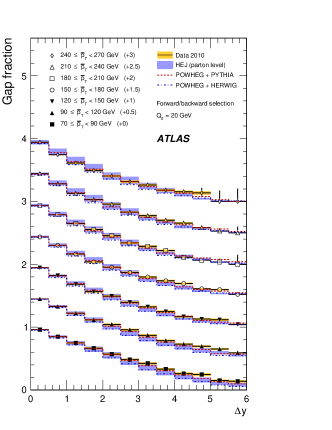
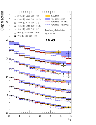
We show in fig. 1 extracts from this ATLAS study, where the gap fraction, defined as the fraction of events with no additional jets in the rapidity region between the two tagging jets, is plotted as a function of $\Delta y$, the difference of the rapidities of the two tagging jets. In the left plot, the tagging jets are defined to be the most forward and most backward jet (in rapidity), while, in the right plot, they are chosen to be the two hardest jets (highest transverse momentum) in each event. In both plots, $\bar{p}_{\mathchoice{\displaystyle}{\scriptstyle}{\scriptscriptstyle}{\scriptscriptstyle}T}$ is the average transverse momentum of the two tagging jets, and results are shown for slices of the average transverse momentum $\overline{p}_{\mathchoice{\displaystyle}{\scriptstyle}{\scriptscriptstyle}{\scriptscriptstyle}T}$ ranging from 70 up to 500 GeV. The experimental data are then compared with the predictions from HEJ [the blue band indicating the scale variation obtained by varying the (equal) renormalization and factorization scale by a factor of 2] and the POWHEG predictions showered by PYTHIA and HERWIG.

We would like to add a few comments to these findings:

1. In the left plot, the theoretical predictions obtained in the two very different approaches of HEJ and POWHEG are very similar and agree with data over a wide range of rapidity intervals and average transverse-momentum slices. For this kinematic quantity, where the tagging jets are selected to be the forward/backward ones, a large hierarchy in the transverse momenta of these jets develops as the average transverse momentum of the forward/backward jets is increased, so that at least one of the forward/backward jets must be very hard. Indeed, it is observed that for this selection, the average difference in the transverse momentum of the forward/backward jet increases systematically with increasing $\Delta y$. Since the veto scale ($Q_{0}$ in the label of the figure) for counting additional jets is much smaller than the average transverse momentum of the tagging jets, the jet production is driven by relatively soft emission from the dijet system. Both HEJ and POWHEG, with different approximations, do include these multiple emissions and lead to similar results and a good agreement with the data.

2. In the right plot of fig. 1, where the tagging jets are chosen to be the two hardest jets in the event, as the average $p_{\mathchoice{\displaystyle}{\scriptstyle}{\scriptscriptstyle}{\scriptscriptstyle}\rm T}$ of the two hardest jets increases to 5 times or more of the veto scale $Q_{0}$, the HEJ prediction starts deviating from data, underestimating the amount of radiation (i.e. the prediction for the gap fraction is larger than the data). This behavior is expected, since the component of events added with naïve tree-level matching increases with increasing $\bar{p}_{\mathchoice{\displaystyle}{\scriptstyle}{\scriptscriptstyle}{\scriptscriptstyle}T}$. This component receives no systematic treatment of soft resummation within HEJ, a situation which would be improved by a complete matching with a parton shower. Progress in this direction has recently been made in ref. Andersen et al. (2011).

   The POWHEG description includes the effects of collinear emissions through the shower formulations, and the theoretical predictions perform well for both kinematic distributions in fig. 1 (particularly when using the PYTHIA shower). However, as can be seen in the right plot, for larger rapidity spans and modest $\bar{p}_{\mathchoice{\displaystyle}{\scriptstyle}{\scriptscriptstyle}{\scriptscriptstyle}T}$, the POWHEG description undershoots the data. Indeed, POWHEG contains no systematic resummation of all the leading-logarithmic terms for large $\Delta y$. Overall, the study reported by ATLAS shows best agreement with the predictions of POWHEG+PYTHIA, but all the studies involve a hierarchy of transverse scales and, therefore, by construction, will favor the description with the systematic collinear resummation of a parton shower.

   Note that the results for POWHEG+HERWIG are consistently below the data (i.e. the events contain too many jets). The differences between the results from POWHEG+PYTHIA and POWHEG+HERWIG should be considered as a theoretical uncertainty connected to the different shower algorithm.

As a final comment, to cleanly separate the two drivers of additional jet activity (a large ratio of transverse scales and a large rapidity separation), it is obviously necessary to use a selection criterion which does not automatically generate a hierarchy in the transverse scales as the rapidity span increases.

II.2 CMS results

CMS has reported a study Chatrchyan et al. (2012) on dijet production with just a simple selection criteria on the transverse momenta of jets. Jets are reconstructed by using the anti-$k_{\mathchoice{\displaystyle}{\scriptstyle}{\scriptscriptstyle}{\scriptscriptstyle}\rm T}$ algorithm with $R=0.5$, and are required to have $p_{\mathchoice{\displaystyle}{\scriptstyle}{\scriptscriptstyle}{\scriptscriptstyle}\rm T}>35$ GeV. Events are then required to contain at least one forward jet ($3.2<|\eta^{f}|<4.7$) and at least one central jet ($|\eta^{c}|<2.8$), where $\eta$ is the pseudorapidity of the jets. The transverse-momentum spectrum of the hardest central and hardest forward jet is then studied, see fig. 2. Obviously, any difference in the two spectra is a result of radiation beyond the tree-level description of back-to-back partons.

Figure 2: The transverse-momentum distributions of the leading forward jet ($3.2<|\eta^{f}|<4.7$) and the leading central jet ($|\eta^{c}|<2.8$) in a sample which requires at least one jet with $p_{\mathchoice{\displaystyle}{\scriptstyle}{\scriptscriptstyle}{\scriptscriptstyle}\rm T}>35$ GeV in each region. The top and bottom row contain the same data points, but different theoretical predictions. The plots are taken from Ref. Chatrchyan et al. (2012).

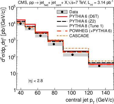
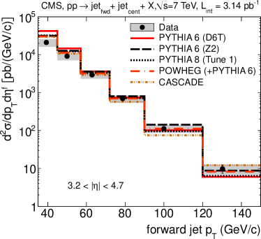
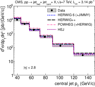
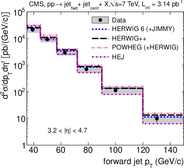
While the CMS study extends the pseudorapidity region of jets up to 4.7 units, the transverse-momentum distributions are integrated over these pseudorapidity ranges. Crucially, however, no large $p_{\mathchoice{\displaystyle}{\scriptstyle}{\scriptscriptstyle}{\scriptscriptstyle}\rm T}$ hierarchy is induced by the cuts, and this gives a cleaner study of the separate effects of the relatively modest rapidity gap.

In the CMS analysis, HEJ describes the $p_{\mathchoice{\displaystyle}{\scriptstyle}{\scriptscriptstyle}{\scriptscriptstyle}\rm T}$ spectrum well for both the central and the forward jets. POWHEG+HERWIG describes the shape correctly, but the normalization is consistently high. The POWHEG+PYTHIA description of the forward jet $p_{\mathchoice{\displaystyle}{\scriptstyle}{\scriptscriptstyle}{\scriptscriptstyle}\rm T}$ distribution performs well, but the description for the central jet shows deviations in both shape and normalization. As the events in this analysis have been specifically selected to have a non-negligible rapidity span, this slight deviation could be attributed to the absence of a systematic treatment of the dominant logarithmic terms for increasing $\Delta\eta$.

II.3 Summary

The analyses discussed so far show that the descriptions of both POWHEG and HEJ are performing well and in broad agreement. The close agreement between the two can, to some extent, be attributed to the requirement of a large $p_{\mathchoice{\displaystyle}{\scriptstyle}{\scriptscriptstyle}{\scriptscriptstyle}\rm T}$ hierarchy in the study by ATLAS or the modest average rapidity spans in the study by CMS.

In the rest of this paper, we investigate various observables which can expose the differences among the fixed NLO calculation, the POWHEG and the HEJ approaches. The first task is therefore to develop a set of cuts for which the NLO prediction for dijet production is physically meaningful. This is the topic of the next section.

III Reliability of the NLO predictions

It has been known for a while that fixed-order results for dijet production are not reliable when symmetric cuts are applied to the transverse momentum of the two hardest jets. This was first noticed in Refs. Klasen and Kramer (1996); Frixione and Ridolfi (1997), in the context of electron-proton collisions at HERA and later also in hadron collisions Andersen et al. (2001). A detailed theoretical discussion of the origin of this fact can be found in Ref. Banfi and Dasgupta (2004), where the next-to-leading-logarithmic resummation of soft logarithms was also performed.

While the fixed-order theoretical predictions display an unphysical behavior as the symmetric-cut limit is reached, the experimental data are obviously not affected by that. Since our goal in the following sections is to find and discuss particular sets of cuts that will allow us to distinguish between the two kinematic regimes implemented in the POWHEG BOX and in HEJ, and since we would like to have a reliable NLO prediction to compare against, in this section we study the reliability of the NLO differential cross sections with several set of cuts, in order to find the most appropriate ones to be used in the following comparisons.

We begin imposing the asymmetric cuts

$$p_{\mathchoice{\displaystyle}{\scriptstyle}{\scriptscriptstyle}{\scriptscriptstyle}\rm T}^{\mathchoice{\displaystyle}{\scriptstyle}{\scriptscriptstyle}{\scriptscriptstyle}j}>p_{\mathchoice{\displaystyle}{\scriptstyle}{\scriptscriptstyle}{\scriptscriptstyle}\rm T}^{\min}\,,\qquad p_{\mathchoice{\displaystyle}{\scriptstyle}{\scriptscriptstyle}{\scriptscriptstyle}\rm T}^{\mathchoice{\displaystyle}{\scriptstyle}{\scriptscriptstyle}{\scriptscriptstyle}j_{1}}>p_{\mathchoice{\displaystyle}{\scriptstyle}{\scriptscriptstyle}{\scriptscriptstyle}\rm T}^{\min}\ +\Delta p_{\mathchoice{\displaystyle}{\scriptstyle}{\scriptscriptstyle}{\scriptscriptstyle}\rm T}\,,\qquad\Delta p_{\mathchoice{\displaystyle}{\scriptstyle}{\scriptscriptstyle}{\scriptscriptstyle}\rm T}>0\,,$$ (1)

i.e. all jets are required to have a minimum transverse momentum $p_{\mathchoice{\displaystyle}{\scriptstyle}{\scriptscriptstyle}{\scriptscriptstyle}\rm T}^{\min}$, while a stronger constraint is applied to the hardest jet in the event, with transverse momentum $p_{\mathchoice{\displaystyle}{\scriptstyle}{\scriptscriptstyle}{\scriptscriptstyle}\rm T}^{\mathchoice{\displaystyle}{\scriptstyle}{\scriptscriptstyle}{\scriptscriptstyle}j_{1}}$. In our notation, $\Delta p_{\mathchoice{\displaystyle}{\scriptstyle}{\scriptscriptstyle}{\scriptscriptstyle}\rm T}$ quantifies then the asymmetry on the cuts. Since in this paper we are interested in studying the size of QCD corrections in regions traditionally used to probe BFKL-like effects, we allow for quite forward jets. Therefore we impose the condition $|y_{j}|<4.7$ on the jet rapidities, and we set $p_{\mathchoice{\displaystyle}{\scriptstyle}{\scriptscriptstyle}{\scriptscriptstyle}\rm T}^{\min}=35$ GeV (similar to the CMS cut discussed in the previous section). Jets are reconstructed by using the anti-$k_{\mathchoice{\displaystyle}{\scriptstyle}{\scriptscriptstyle}{\scriptscriptstyle}\rm T}$ jet algorithm Cacciari et al. (2008) with $R=0.5$ and $E-$scheme recombination. The NLO results, as well as the POWHEG distributions shown in section IV, have been obtained with renormalization and factorization scales set to the POWHEG underlying-Born transverse momentum, i.e. the $p_{\mathchoice{\displaystyle}{\scriptstyle}{\scriptscriptstyle}{\scriptscriptstyle}\rm T}$ of the partons in the Born-like $2\to 2$ kinematics, the starting point for the generation of radiation Alioli et al. (2011). For all the plots in the paper we have used the MSTW2008 Martin et al. (2009) parton distribution function set. The aim of this section is to explore several sets of cuts to be applied to the jets and to clarify the breaking point, where the NLO calculation becomes unreliable.

Figure 3: The dependence of the $d\sigma/d\Delta y_{\mathchoice{\displaystyle}{\scriptstyle}{\scriptscriptstyle}{\scriptscriptstyle}\rm fb}$ distribution on the asymmetry of jet cuts (left plot) and of the total cross section in different $\Delta y_{\mathchoice{\displaystyle}{\scriptstyle}{\scriptscriptstyle}{\scriptscriptstyle}\rm fb}$ slices, as a function of the jet cuts asymmetry $\Delta p_{\mathchoice{\displaystyle}{\scriptstyle}{\scriptscriptstyle}{\scriptscriptstyle}\rm T}$ (right plot).

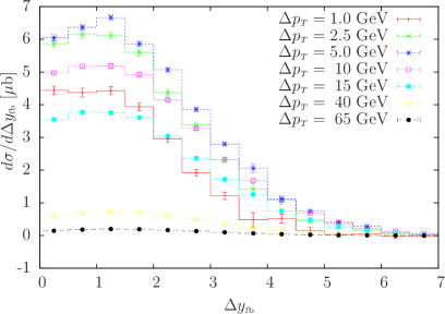
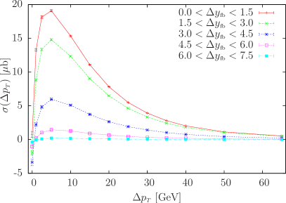
In fig. 3, we illustrate the effects of the cuts of eq. (1): in the left plot, we display the differential cross section for dijet inclusive production as a function of $\Delta y_{\mathchoice{\displaystyle}{\scriptstyle}{\scriptscriptstyle}{\scriptscriptstyle}\rm fb}$, the difference in rapidity of the most forward and most backward jet. The various curves correspond to different values of $\Delta p_{\mathchoice{\displaystyle}{\scriptstyle}{\scriptscriptstyle}{\scriptscriptstyle}\rm T}$ in eq. (1), ranging from $\Delta p_{\mathchoice{\displaystyle}{\scriptstyle}{\scriptscriptstyle}{\scriptscriptstyle}\rm T}=1$ GeV up to $\Delta p_{\mathchoice{\displaystyle}{\scriptstyle}{\scriptscriptstyle}{\scriptscriptstyle}\rm T}=65$ GeV. On physical grounds, we expect a decrease of the differential cross section as $\Delta p_{\mathchoice{\displaystyle}{\scriptstyle}{\scriptscriptstyle}{\scriptscriptstyle}\rm T}$ increases. However we observe that the NLO results do not show this behaviour. Indeed, over a wide range in $\Delta y_{\mathchoice{\displaystyle}{\scriptstyle}{\scriptscriptstyle}{\scriptscriptstyle}\rm fb}$, the cross sections increase for increasing $\Delta p_{\mathchoice{\displaystyle}{\scriptstyle}{\scriptscriptstyle}{\scriptscriptstyle}\rm T}$ until a maximum is reached at $\Delta p_{\mathchoice{\displaystyle}{\scriptstyle}{\scriptscriptstyle}{\scriptscriptstyle}\rm T}\approx 5$ GeV. Then, for any further increase of $\Delta p_{\mathchoice{\displaystyle}{\scriptstyle}{\scriptscriptstyle}{\scriptscriptstyle}\rm T}$, the cross section decreases, as expected. The unphysical behaviour for small $\Delta p_{\mathchoice{\displaystyle}{\scriptstyle}{\scriptscriptstyle}{\scriptscriptstyle}\rm T}$ is caused by a large logarithmic term in $\Delta p_{\mathchoice{\displaystyle}{\scriptstyle}{\scriptscriptstyle}{\scriptscriptstyle}\rm T}$, arising from a suppression in the emission of radiation above the $\Delta p_{\mathchoice{\displaystyle}{\scriptstyle}{\scriptscriptstyle}{\scriptscriptstyle}\rm T}$ scale, which causes uncancelled virtual corrections to build up above this scale. The same behaviour is also evident in the right plot of fig. 3, where the cross section is plotted against $\Delta p_{\mathchoice{\displaystyle}{\scriptstyle}{\scriptscriptstyle}{\scriptscriptstyle}\rm T}$ for various slices in $\Delta y_{\mathchoice{\displaystyle}{\scriptstyle}{\scriptscriptstyle}{\scriptscriptstyle}\rm fb}$. The presence of uncanceled virtual corrections becomes manifest for small $\Delta p_{\mathchoice{\displaystyle}{\scriptstyle}{\scriptscriptstyle}{\scriptscriptstyle}\rm T}$, where the cross section is unphysically negative.

Figure 4: The differential cross sections $d\sigma/d\Delta y_{\mathchoice{\displaystyle}{\scriptstyle}{\scriptscriptstyle}{\scriptscriptstyle}\rm fb}$ for several values of $p_{\mathchoice{\displaystyle}{\scriptstyle}{\scriptscriptstyle}{\scriptscriptstyle}\rm T}^{*}$ at $X=2/3$ (left plot) and for several values of $X$ for $p_{\mathchoice{\displaystyle}{\scriptstyle}{\scriptscriptstyle}{\scriptscriptstyle}\rm T}^{*}=75$ GeV (right plot). For both plots, jets have transverse momentum greater than 35 GeV.

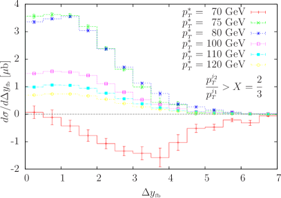
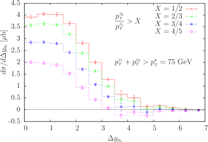
In fig. 4, we plot the differential cross section as a function of $\Delta y_{\mathchoice{\displaystyle}{\scriptstyle}{\scriptscriptstyle}{\scriptscriptstyle}\rm fb}$ using another set of cuts, BFKL-inspired:

$$p_{\mathchoice{\displaystyle}{\scriptstyle}{\scriptscriptstyle}{\scriptscriptstyle}\rm T}^{\mathchoice{\displaystyle}{\scriptstyle}{\scriptscriptstyle}{\scriptscriptstyle}j}>p_{\mathchoice{\displaystyle}{\scriptstyle}{\scriptscriptstyle}{\scriptscriptstyle}\rm T}^{\min}=35~{}{\rm GeV}\,,\qquad p_{\mathchoice{\displaystyle}{\scriptstyle}{\scriptscriptstyle}{\scriptscriptstyle}\rm T}^{\mathchoice{\displaystyle}{\scriptstyle}{\scriptscriptstyle}{\scriptscriptstyle}j_{1}}+p_{\mathchoice{\displaystyle}{\scriptstyle}{\scriptscriptstyle}{\scriptscriptstyle}\rm T}^{\mathchoice{\displaystyle}{\scriptstyle}{\scriptscriptstyle}{\scriptscriptstyle}j_{2}}>p_{\mathchoice{\displaystyle}{\scriptstyle}{\scriptscriptstyle}{\scriptscriptstyle}\rm T}^{*}\,,\qquad\frac{p_{\mathchoice{\displaystyle}{\scriptstyle}{\scriptscriptstyle}{\scriptscriptstyle}\rm T}^{\mathchoice{\displaystyle}{\scriptstyle}{\scriptscriptstyle}{\scriptscriptstyle}j_{2}}}{p_{\mathchoice{\displaystyle}{\scriptstyle}{\scriptscriptstyle}{\scriptscriptstyle}\rm T}^{\mathchoice{\displaystyle}{\scriptstyle}{\scriptscriptstyle}{\scriptscriptstyle}j_{1}}}>X\,,\qquad|y_{j}|<4.7\,,$$ (2)

where $j_{1}$ and $j_{2}$ denote the hardest and next-to-hardest jet, respectively. In the left plot of fig. 4, we show the cross sections obtained at a fixed value of $X$ (chosen here to be $2/3$) for several values of $p_{\mathchoice{\displaystyle}{\scriptstyle}{\scriptscriptstyle}{\scriptscriptstyle}\rm T}^{*}$ . The rôle of $\Delta p_{\mathchoice{\displaystyle}{\scriptstyle}{\scriptscriptstyle}{\scriptscriptstyle}\rm T}$ in fig. 3 is now played by the distance $p_{\mathchoice{\displaystyle}{\scriptstyle}{\scriptscriptstyle}{\scriptscriptstyle}\rm T}^{*}-2\,p_{\mathchoice{\displaystyle}{\scriptstyle}{\scriptscriptstyle}{\scriptscriptstyle}\rm T}^{\min}$. In fact, when $p_{\mathchoice{\displaystyle}{\scriptstyle}{\scriptscriptstyle}{\scriptscriptstyle}\rm T}^{*}$ reaches its minimum value equal to $2\,p_{\mathchoice{\displaystyle}{\scriptstyle}{\scriptscriptstyle}{\scriptscriptstyle}\rm T}^{\min}$, jets can approach the symmetric-cut configuration, exposing again large logarithms in a fixed NLO calculation. The red curve shows precisely the unphysical behavior when $p_{\mathchoice{\displaystyle}{\scriptstyle}{\scriptscriptstyle}{\scriptscriptstyle}\rm T}^{*}=2\,p_{\mathchoice{\displaystyle}{\scriptstyle}{\scriptscriptstyle}{\scriptscriptstyle}\rm T}^{\min}=70$ GeV, giving rise to a negative cross section. We have checked that this conclusion holds regardless of the value of $X$ chosen. As $p_{\mathchoice{\displaystyle}{\scriptstyle}{\scriptscriptstyle}{\scriptscriptstyle}\rm T}^{*}$ increases beyond its minimal value, the cross sections exhibit a physical behavior, i.e. they decrease. In the right plot of fig. 4, we display the differential cross sections for $p_{\mathchoice{\displaystyle}{\scriptstyle}{\scriptscriptstyle}{\scriptscriptstyle}\rm T}^{*}=75$ GeV and for several values of $X$. The symmetric-cut regime is here reached when $X\to 1$, and in fact, as the values of $X$ increases, the differential cross sections develop negative tails for high $\Delta y_{\mathchoice{\displaystyle}{\scriptstyle}{\scriptscriptstyle}{\scriptscriptstyle}\rm fb}$.

Figure 5: Cross sections for different slices in $\Delta y_{\mathchoice{\displaystyle}{\scriptstyle}{\scriptscriptstyle}{\scriptscriptstyle}\rm fb}$ as a function of $p_{\mathchoice{\displaystyle}{\scriptstyle}{\scriptscriptstyle}{\scriptscriptstyle}\rm T}^{*}$ at $X=2/3$ (left plot) and as a function of $X$ at $p_{\mathchoice{\displaystyle}{\scriptstyle}{\scriptscriptstyle}{\scriptscriptstyle}\rm T}^{*}=75$ GeV (right plot).

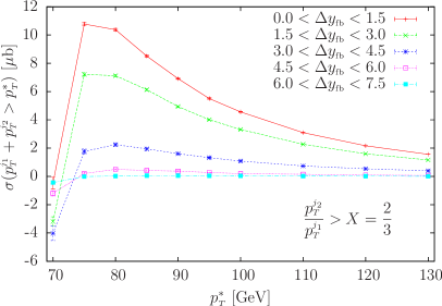
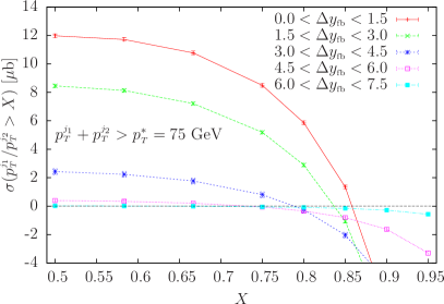
The two plots in fig. 5, and similar ones that can be drawn for other values of $X$ and $p_{\mathchoice{\displaystyle}{\scriptstyle}{\scriptscriptstyle}{\scriptscriptstyle}\rm T}^{*}$, can help in the not-easy task of establishing what cuts to apply in an analysis if one wants to compare the experimental data to the NLO calculation using the alternative cuts of eq. (2). In the left plot, the cross sections plotted for several slices in $\Delta y_{\mathchoice{\displaystyle}{\scriptstyle}{\scriptscriptstyle}{\scriptscriptstyle}\rm fb}$ become negative for values of $p_{\mathchoice{\displaystyle}{\scriptstyle}{\scriptscriptstyle}{\scriptscriptstyle}\rm T}^{*}$ less than 75 GeV, fixing then a lower value below which the theoretical distributions cannot be trusted. Similarly, the right plot, where the cross sections are plotted as a function of $X$ at a fixed value of $p_{\mathchoice{\displaystyle}{\scriptstyle}{\scriptscriptstyle}{\scriptscriptstyle}\rm T}^{*}=75$ GeV, gives an indication of the upper value of $X$ above which the NLO predictions become unreliable, for different slices of $\Delta y_{\mathchoice{\displaystyle}{\scriptstyle}{\scriptscriptstyle}{\scriptscriptstyle}\rm fb}$.

IV Probing higher-order corrections: a comparison among POWHEG, HEJ and NLO results

We are now in a position to compare three theoretical approaches to dijet production that include higher-order effects: NLO, POWHEG and HEJ. The aim of this section is to investigate a number of observables based on hard jets, which could better expose the differences between the description obtained in the three approaches.

In order to avoid biasing our event sample towards a large hierarchy of transverse scale, we impose a minimal set of asymmetric cuts (as discussed around eq. 3)

$$p_{\mathchoice{\displaystyle}{\scriptstyle}{\scriptscriptstyle}{\scriptscriptstyle}\rm T}^{\mathchoice{\displaystyle}{\scriptstyle}{\scriptscriptstyle}{\scriptscriptstyle}j}>35\ {\rm GeV},\quad p_{\mathchoice{\displaystyle}{\scriptstyle}{\scriptscriptstyle}{\scriptscriptstyle}\rm T}^{\mathchoice{\displaystyle}{\scriptstyle}{\scriptscriptstyle}{\scriptscriptstyle}j_{1}}>45\ {\rm GeV},\quad|y_{j}|<4.7\,,$$ (3)

i.e. all jets are required to have a minimum transverse momentum of 35 GeV, and the hardest-jet transverse momentum, $p_{\mathchoice{\displaystyle}{\scriptstyle}{\scriptscriptstyle}{\scriptscriptstyle}\rm T}^{\mathchoice{\displaystyle}{\scriptstyle}{\scriptscriptstyle}{\scriptscriptstyle}j_{1}}$, is required to be greater than 45 GeV. In order to comply with the experimental acceptance, all jets are further required to have an absolute rapidity $|y_{j}|$ less than 4.7. Jets are defined according to the anti-$k_{\mathchoice{\displaystyle}{\scriptstyle}{\scriptscriptstyle}{\scriptscriptstyle}\rm T}$ jet algorithm, with radius $R=0.5$. Only events with at least two jets fulfilling eq. (3) are kept. We stress that neither the POWHEG nor the HEJ descriptions exhibit the unphysical behaviour of the NLO result when using symmetric cuts, since they include a partial resummation of the large logarithmic terms. However, in order to have a meaningful NLO prediction to compare with, we must impose asymmetric cuts.

In the following, we compare the cross sections computed with a fixed NLO calculation and with HEJ, with the results obtained analyzing 14M events generated by the POWHEG BOX, at the level of the first-emission and after the shower performed by PYTHIA . The renormalization and factorization scales have been chosen equal to the transverse momentum of the hardest jet in each event, for the HEJ predictions. For the NLO computation (and for computing the POWHEG $\bar{B}$ function), scales are set to the transverse momentum of the underlying-Born configuration, as in the previous section. Scale-uncertainty bands, obtained by varying these scales by a factor of 2 in each direction, are shown for the NLO and HEJ results. The scales entering in the evaluation of parton distribution functions and of the strong coupling in the POWHEG Sudakov form factor are instead evaluated with a scale equal to the transverse momentum of the POWHEG hardest emission Frixione et al. (2007); Alioli et al. (2011).

The statistical errors (due to the numerical integration of the differential cross sections) on the theoretical predictions for the ratios studied in this section have been computed with the standard propagation of errors for the ratio of two uncorrelated quantities. We expect these errors to be an overestimation of the true ones, since, in our case, the numerator and denominator are strongly correlated.

Figure 6: The average number of jets as a function of $\Delta y_{\rm fb}$ (top left plot) and of $H_{\mathchoice{\displaystyle}{\scriptstyle}{\scriptscriptstyle}{\scriptscriptstyle}\rm T}$ (bottom left plot), as predicted by a fixed NLO calculation, by POWHEG first emission, by POWHEG+PYTHIA and by HEJ. The dotted red lines around the HEJ prediction and the green ones around the NLO result are obtained by varying the renormalization and factorization scales by a factor of 2 around their central value. The right plot (from Ref. Aad et al. (2011a)) shows the average number of additional jets as found in the analysis from ATLAS.

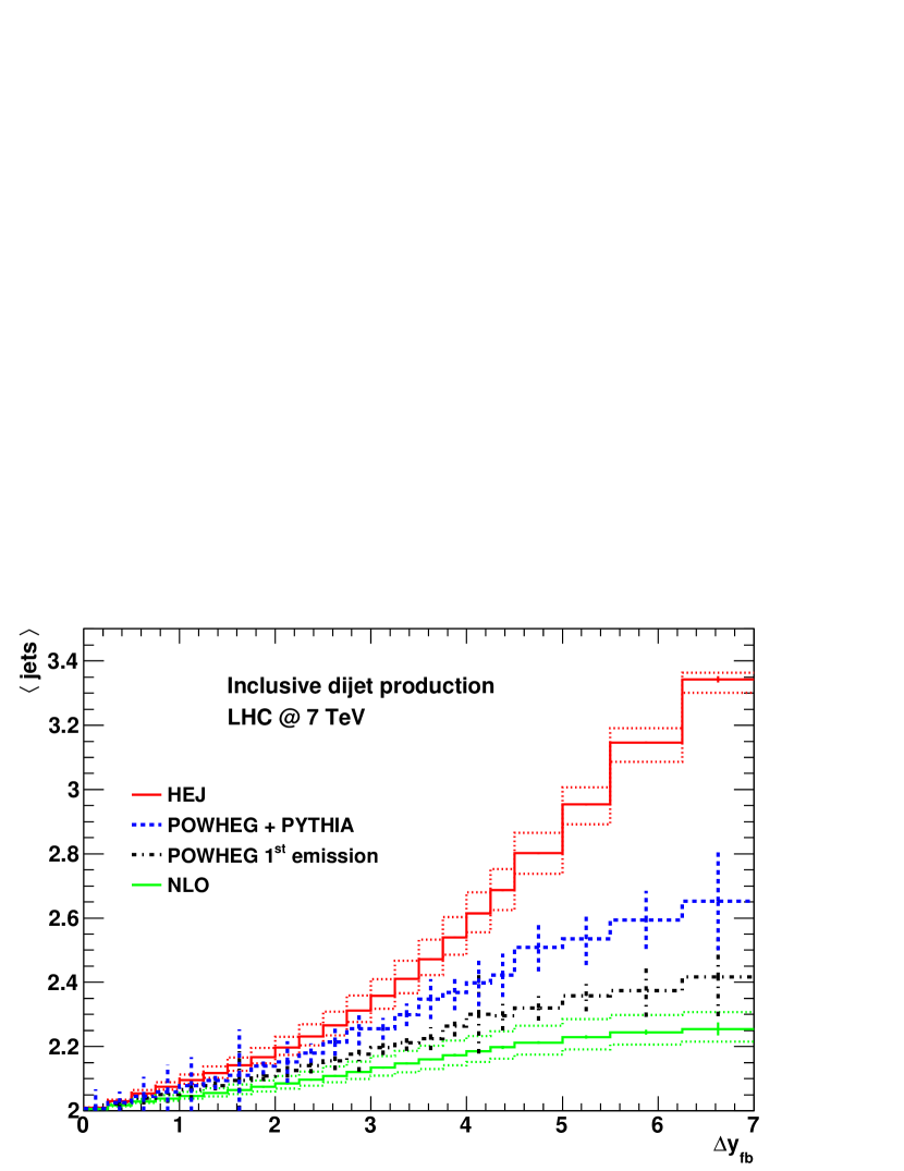
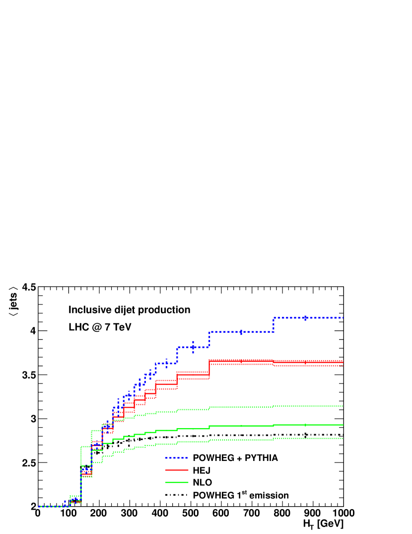
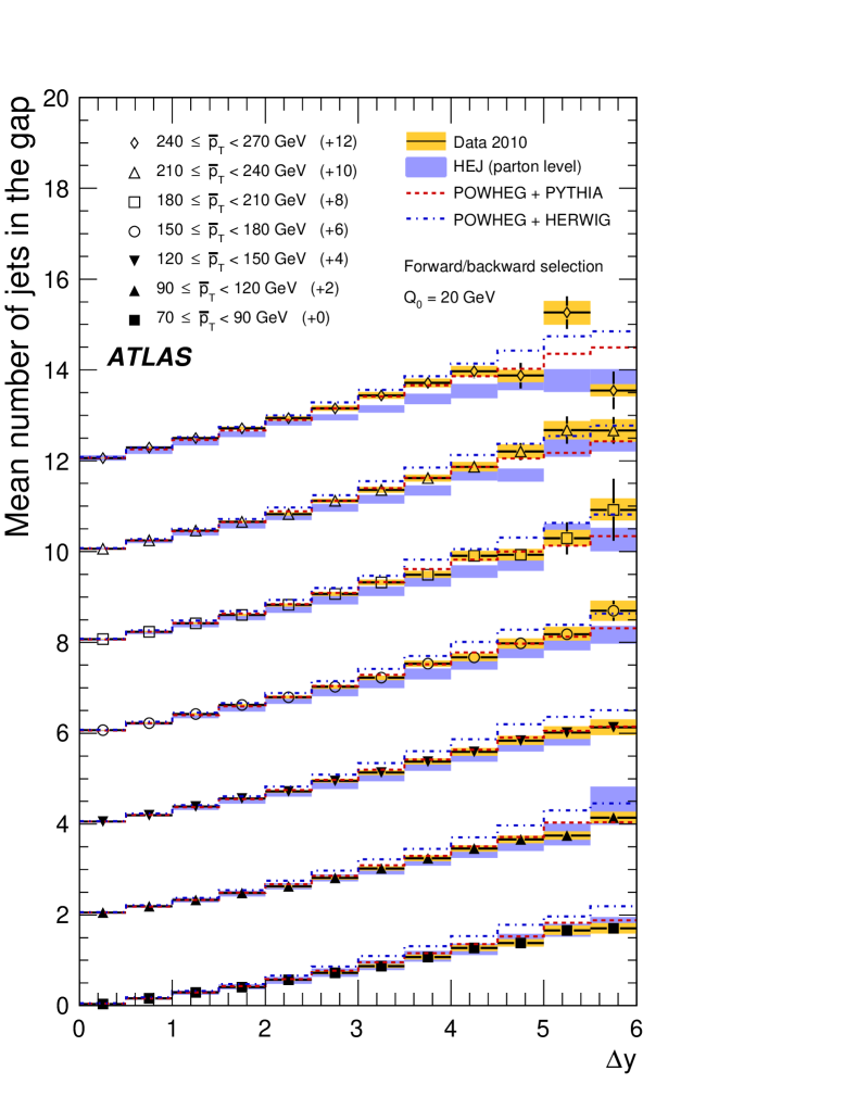
In fig. 6, we plot on the top left the average number of jets as a function of the rapidity difference $\Delta y_{\mathchoice{\displaystyle}{\scriptstyle}{\scriptscriptstyle}{\scriptscriptstyle}\rm fb}$ between the most forward and most backward of the jets fulfilling eq. (3) and the same quantity as a function of $H_{\mathchoice{\displaystyle}{\scriptstyle}{\scriptscriptstyle}{\scriptscriptstyle}\rm T}=\sum_{j}p_{\mathchoice{\displaystyle}{\scriptstyle}{\scriptscriptstyle}{\scriptscriptstyle}\rm T}^{\mathchoice{\displaystyle}{\scriptstyle}{\scriptscriptstyle}{\scriptscriptstyle}j}$ at the bottom left. To ease the comparison, we also show the result of the jet activity between the gap as a function of $\Delta y_{\mathchoice{\displaystyle}{\scriptstyle}{\scriptscriptstyle}{\scriptscriptstyle}\rm fb}$ in the analysis by ATLAS Aad et al. (2011a) to the right of the same figure. The analysis suggested in the present paper clearly shows more discriminating power between the results of POWHEG and HEJ than the one of Ref. Aad et al. (2011a).

As far as the dependence on $\Delta y_{\mathchoice{\displaystyle}{\scriptstyle}{\scriptscriptstyle}{\scriptscriptstyle}\rm fb}$ is concerned, the wide-angle resummation implemented in HEJ produces more hard jets than POWHEG and the fixed NLO calculation, as $\Delta y_{\mathchoice{\displaystyle}{\scriptstyle}{\scriptscriptstyle}{\scriptscriptstyle}\rm fb}$ increases. Both the NLO and the first-emission POWHEG results have at most 3 jets, so that the average number of jets cannot exceed 3, and are in good agreement. Additional jets are instead produced by the PYTHIA shower, so that the average number of jets is increased by roughly 20% with respect to the NLO one, for $\Delta y_{\rm fb}\approx 7$. For the same separation in rapidity, the HEJ prediction is 45% larger than the NLO result, with a chance to distinguish among the three approaches. While this variable is related to the gap fraction discussed previously, it is more exclusive as it is sensitive to the number of jets in each event and not just whether a 3rd jet exists. We therefore anticipate greater distinguishing power between the different theoretical approaches. This same distribution has been investigated also in the analysis by ATLAS Aad et al. (2011a), but, as discussed earlier, the cuts applied in that analysis [in contrast to eq. (3)] enhance the effects of collinear emissions, which are treated to leading-logarithmic order in POWHEG and partly in HEJ.

The scale variation (dotted lines around the NLO and HEJ curves) are modest, of the order of a few percent. As a final comment, we note that the prediction from HEJ was found to be very stable against the effects of further showering Andersen et al. (2011) [by using cuts very similar to those in eq. (3)].

The dependence of the average number of jets on $H_{\mathchoice{\displaystyle}{\scriptstyle}{\scriptscriptstyle}{\scriptscriptstyle}\rm T}$ (bottom left plot in fig. 6) displays a different behaviour: here the showered events have, on average, more jets than HEJ and the NLO results, as the sum of the transverse momentum of all the final-state jets increases. It is interesting here to comment on the NLO result obtained with the factorization and renormalization scales set to $p_{\mathchoice{\displaystyle}{\scriptstyle}{\scriptscriptstyle}{\scriptscriptstyle}\rm T}^{\rm\scriptscriptstyle UB}/2$, half of the transverse momentum of the underlying-Born configuration, i.e. the upper green dotted line in the plot. In fact, this quantity is greater than 3, for $H_{\mathchoice{\displaystyle}{\scriptstyle}{\scriptscriptstyle}{\scriptscriptstyle}\rm T}\gtrsim 270$ GeV, which in a NLO calculation signals the fact that the two-jet exclusive cross section becomes negative. We will comment on this after the discussion of fig. 7 that suffers from the same problem.

Figure 7: Ratio of the inclusive three-jet rate over the inclusive two-jet one, as a function of $\Delta y_{\mathchoice{\displaystyle}{\scriptstyle}{\scriptscriptstyle}{\scriptscriptstyle}\rm fb}$ (left plot) and $H_{\mathchoice{\displaystyle}{\scriptstyle}{\scriptscriptstyle}{\scriptscriptstyle}T2}$ (right plot). The dotted lines display the results obtained by varying the renormalization and factorization scales by a factor of 2 around the central value, for the HEJ (red) and NLO (green) predictions.

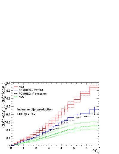
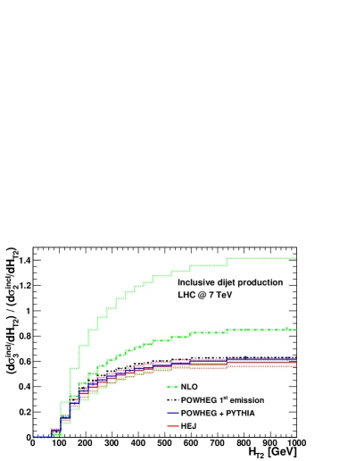
In fig. 7, we plot the ratio of the three-jet inclusive cross section over the two-jet one, as a function of $\Delta y_{\rm\mathchoice{\displaystyle}{\scriptstyle}{\scriptscriptstyle}{\scriptscriptstyle}fb}$ (left plot) and as a function of $H_{\mathchoice{\displaystyle}{\scriptstyle}{\scriptscriptstyle}{\scriptscriptstyle}T2}$ (right plot), where $H_{\mathchoice{\displaystyle}{\scriptstyle}{\scriptscriptstyle}{\scriptscriptstyle}T2}=p_{\mathchoice{\displaystyle}{\scriptstyle}{\scriptscriptstyle}{\scriptscriptstyle}\rm T}^{\mathchoice{\displaystyle}{\scriptstyle}{\scriptscriptstyle}{\scriptscriptstyle}j_{1}}+p_{\mathchoice{\displaystyle}{\scriptstyle}{\scriptscriptstyle}{\scriptscriptstyle}\rm T}^{\mathchoice{\displaystyle}{\scriptstyle}{\scriptscriptstyle}{\scriptscriptstyle}j_{2}}$ is the sum of the transverse momenta of the two hardest jets in the event. The same comments made about the top left plot of fig. 6 apply here: the BFKL-inspired resummation implemented by HEJ produces more hard jets than the resummation of the parton shower of POWHEG+PYTHIA, for large rapidity separation between the most forward and most backward jet. For this distribution, an experimental analysis should then be able to distinguish between the HEJ and the POWHEG+PYTHIA predictions, even though the observable is less exclusive than the average number of jets (and directly related to the gap fraction studied by ATLAS).

In the right plot, the NLO ratio for the three-jet inclusive cross section over the two-jet one, plotted as a function of $H_{\mathchoice{\displaystyle}{\scriptstyle}{\scriptscriptstyle}{\scriptscriptstyle}T2}$, becomes unphysical (i.e. it becomes greater than 1) when the factorization and renormalization scales are set to $p_{\mathchoice{\displaystyle}{\scriptstyle}{\scriptscriptstyle}{\scriptscriptstyle}\rm T}^{\rm\mathchoice{\displaystyle}{\scriptstyle}{\scriptscriptstyle}{\scriptscriptstyle}UB}/2$, for higher values of $H_{\mathchoice{\displaystyle}{\scriptstyle}{\scriptscriptstyle}{\scriptscriptstyle}T2}$. This result is linked with the same unreliable behavior of the NLO distribution in the bottom left plot of fig. 6 and deserves an explanation that we give in Appendix A. The predictions from HEJ and POWHEG+PYTHIA are in remarkably good agreement, both close to the POWHEG first-emission result, implying that the first POWHEG emission has the strongest impact on this distribution, while the subsequent shower has a milder effect. Before leaving this discussion, we would like to point out that, when using the cuts reported by the ATLAS Collaboration Aad et al. (2011b)

$$p_{\mathchoice{\displaystyle}{\scriptstyle}{\scriptscriptstyle}{\scriptscriptstyle}\rm T}^{\mathchoice{\displaystyle}{\scriptstyle}{\scriptscriptstyle}{\scriptscriptstyle}j}>60\ {\rm GeV},\quad p_{\mathchoice{\displaystyle}{\scriptstyle}{\scriptscriptstyle}{\scriptscriptstyle}\rm T}^{\mathchoice{\displaystyle}{\scriptstyle}{\scriptscriptstyle}{\scriptscriptstyle}j_{1}}>80\ {\rm GeV},\quad|y_{j}|<2.8\,,$$ (4)

no significant difference is generated between the NLO result and the other three curves (in complete agreement with the results reported in Ref. Aad et al. (2011b)).

Figure 8: The average value of $\cos(\pi-\phi_{\rm\mathchoice{\displaystyle}{\scriptstyle}{\scriptscriptstyle}{\scriptscriptstyle}fb})$ as a function of $\Delta y_{\rm\mathchoice{\displaystyle}{\scriptstyle}{\scriptscriptstyle}{\scriptscriptstyle}fb}$, where $\phi_{\rm\mathchoice{\displaystyle}{\scriptstyle}{\scriptscriptstyle}{\scriptscriptstyle}fb}$ is the azimuthal angle separation between the most forward and most backward jet. The dotted red and green lines are obtained by varying the renormalization and factorization scales by a factor of 2 in both directions around the central value.

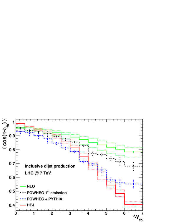
As a last example of a kinematic distribution that displays different behaviour if evaluated at NLO or by using POWHEG or HEJ, we plot, in fig. 8, the average value of $\cos(\pi-\phi_{\rm\mathchoice{\displaystyle}{\scriptstyle}{\scriptscriptstyle}{\scriptscriptstyle}fb})$, where $\phi_{\rm\mathchoice{\displaystyle}{\scriptstyle}{\scriptscriptstyle}{\scriptscriptstyle}fb}$ is the azimuthal angle between the most forward and backward jets, as a function of their rapidity separation $\Delta y_{\rm\mathchoice{\displaystyle}{\scriptstyle}{\scriptscriptstyle}{\scriptscriptstyle}fb}$. For dijet events at tree level, $\phi_{\rm\mathchoice{\displaystyle}{\scriptstyle}{\scriptscriptstyle}{\scriptscriptstyle}fb}=\pi$, since the two jets are back-to-back, and the average value of the cosine is 1. Deviation from 1 then indicates the presence of additional emissions, so that this kinematic distribution carries information on the decorrelation between the two jets. This observable has been promoted for a long time as a good discriminator between descriptions with and without a systematic evolution in rapidity. It has therefore also been studied with a full detector simulation in ref. d’Enterria (2009). However, the striking prediction from pure leading-logarithmic BFKL evolution of an azimuthal decorrelation much larger than that which is obtained in a parton shower or fixed-order formulation has been brought into question for some time by the inclusion of subleading corrections Orr and Stirling (1997); Colferai et al. (2010). This quantity is more inclusive than the average number of jets, as it is sensitive also to emissions below the jet $p_{\mathchoice{\displaystyle}{\scriptstyle}{\scriptscriptstyle}{\scriptscriptstyle}\rm T}$ cut. The higher radiation activity in POWHEG+PYTHIA and in HEJ, with respect to the fixed NLO and the POWHEG first-emission results, is clearly visible in the figure: the stronger jet activity produced by HEJ at higher rapidity separation (see the left plot of fig. 6) lowers the average value of the cosine below the POWHEG+PYTHIA result. As expected, the average value predicted by the POWHEG first-emission and the NLO calculation is closer to 1, since they contain at most one radiated parton. At large rapidity separations, the prediction from dijets at NLO is of significantly less decorelation than that from either POWHEG+PYTHIA or HEJ.

Concluding the study of distributions we note that when the average number of jets is analysed vs the hardness of the event measured as $H_{T}$ and the ordering of predictions from fewer to more hard jets is NLO, HEJ, POWHEG+PYTHIA. In the more inclusive analysis of the three-jet rate over the two-jet rate vs $H_{T2}$, the results of POWHEG+PYTHIA and HEJ are very similar, and the NLO prediction is of just a slightly larger share of inclusive three-jet events.

However, when the additional jet activity is studied as a function of the rapidity separation between the most forward/backward jets, then the results of the perturbative predictions are systematically ordered from least to most radiation as: NLO, POWHEG+PYTHIA and HEJ. This is seen in fig. 6 for the average number of jets and in fig. 7 for the inclusive three-jet rate over the inclusive two-jet rate. We can thus confirm that the a priori expected behaviour between the various perturbative frameworks is indeed realized in practice.

V Conclusions

Recent analyses by the ATLAS and the CMS Collaborations of inclusive and exclusive dijet production showed a high level of agreement between the two very different approaches to the description of perturbative higher-order corrections implemented in the POWHEG BOX and in HEJ, within the specific cuts and analyses applied.

Inspired by these results, we have presented an analysis developed to clearly display the differences in the radiation patterns arising in a fixed NLO calculation, HEJ and POWHEG+PYTHIA. All the observables discussed probe directly the further radiation from a dijet system, so the NLO calculation of dijet production is the lowest order nontrivial prediction for the observable.

While the limitations of the NLO calculation are clearly visible when probing regions of the phase space where multijet emissions become important, we have shown also that the predictions of POWHEG+PYTHIA and HEJ are clearly distinguishable for the average number of jets and the ratio of the inclusive three-jet production over the inclusive two-jet production, when studied as a function of the rapidity separation of the most forward and the most backward jet. Less marked differences are found when these quantities are plotted as a function of the sum of the transverse momenta of all the jets, or as a function of the transverse momenta of the two leading jets. Contrary to these findings, the study of the azimuthal decorrelation of the most forward and backward jet turned out to be less promising in distinguishing the two descriptions given by POWHEG and HEJ - while effects beyond pure NLO should be clearly visible.

We hope that an experimental measurement of dijet data collected at the LHC based on the suggestions presented in this paper will follow, in order to investigate the quality of the theoretical understanding of these kinematic distributions.

Appendix A The exclusive two-jet cross section

In this appendix we give an explanation of the unphysical behavior of the NLO distributions shown in the bottom left plot of fig. 6 and in the right plot in fig. 7, when the factorization and renormalization scales are set to $p_{\mathchoice{\displaystyle}{\scriptstyle}{\scriptscriptstyle}{\scriptscriptstyle}\rm T}^{\rm\mathchoice{\displaystyle}{\scriptstyle}{\scriptscriptstyle}{\scriptscriptstyle}UB}/2$. For ease of notation we introduce the following shortcuts

$$\tilde{\sigma}_{2}^{\mathchoice{\displaystyle}{\scriptstyle}{\scriptscriptstyle}{\scriptscriptstyle}\rm incl}=\frac{d\sigma_{2}^{\rm\mathchoice{\displaystyle}{\scriptstyle}{\scriptscriptstyle}{\scriptscriptstyle}incl}}{dH_{\mathchoice{\displaystyle}{\scriptstyle}{\scriptscriptstyle}{\scriptscriptstyle}T2}}\,,\qquad\quad\tilde{\sigma}_{3}^{\mathchoice{\displaystyle}{\scriptstyle}{\scriptscriptstyle}{\scriptscriptstyle}\rm incl}=\frac{d\sigma_{3}^{\rm\mathchoice{\displaystyle}{\scriptstyle}{\scriptscriptstyle}{\scriptscriptstyle}incl}}{dH_{\mathchoice{\displaystyle}{\scriptstyle}{\scriptscriptstyle}{\scriptscriptstyle}T2}}\,,$$ (5)

where the lower index 2 or 3 indicates the number of jets and the differential cross sections are inclusive with respect to the corresponding number of jets. Together with inclusive cross sections, we define the exclusive ones, that will be designated with the upper label “excl”. At fixed NLO, in dijet production, we have

$$\tilde{\sigma}_{3}^{\mathchoice{\displaystyle}{\scriptstyle}{\scriptscriptstyle}{\scriptscriptstyle}\rm incl}=\tilde{\sigma}_{3}^{\mathchoice{\displaystyle}{\scriptstyle}{\scriptscriptstyle}{\scriptscriptstyle}\rm excl}\,,\qquad\quad\tilde{\sigma}_{2}^{\mathchoice{\displaystyle}{\scriptstyle}{\scriptscriptstyle}{\scriptscriptstyle}\rm incl}=\tilde{\sigma}_{2}^{\mathchoice{\displaystyle}{\scriptstyle}{\scriptscriptstyle}{\scriptscriptstyle}\rm excl}+\tilde{\sigma}_{3}^{\mathchoice{\displaystyle}{\scriptstyle}{\scriptscriptstyle}{\scriptscriptstyle}\rm excl}\,,$$ (6)

and we can relate the average number of jets with the inclusive three-jet over two-jet ratio

$$\langle{\rm jets}\rangle\equiv\frac{2\,\tilde{\sigma}_{2}^{\mathchoice{\displaystyle}{\scriptstyle}{\scriptscriptstyle}{\scriptscriptstyle}\rm excl}+3\,\tilde{\sigma}_{3}^{\mathchoice{\displaystyle}{\scriptstyle}{\scriptscriptstyle}{\scriptscriptstyle}\rm excl}}{\tilde{\sigma}_{2}^{\mathchoice{\displaystyle}{\scriptstyle}{\scriptscriptstyle}{\scriptscriptstyle}\rm excl}+\tilde{\sigma}_{3}^{\mathchoice{\displaystyle}{\scriptstyle}{\scriptscriptstyle}{\scriptscriptstyle}\rm excl}}=2+\frac{\tilde{\sigma}_{3}^{\mathchoice{\displaystyle}{\scriptstyle}{\scriptscriptstyle}{\scriptscriptstyle}\rm excl}}{\tilde{\sigma}_{2}^{\mathchoice{\displaystyle}{\scriptstyle}{\scriptscriptstyle}{\scriptscriptstyle}\rm incl}}=2+\frac{\tilde{\sigma}_{3}^{\mathchoice{\displaystyle}{\scriptstyle}{\scriptscriptstyle}{\scriptscriptstyle}\rm incl}}{\tilde{\sigma}_{2}^{\mathchoice{\displaystyle}{\scriptstyle}{\scriptscriptstyle}{\scriptscriptstyle}\rm incl}}$$ (7)

so that the two unphysical behaviors of the right plots in figs. 6 and 7 are strictly connected. The ratio

$$\frac{\tilde{\sigma}_{3}^{\mathchoice{\displaystyle}{\scriptstyle}{\scriptscriptstyle}{\scriptscriptstyle}\rm incl}}{\tilde{\sigma}_{2}^{\mathchoice{\displaystyle}{\scriptstyle}{\scriptscriptstyle}{\scriptscriptstyle}\rm incl}}=\frac{\tilde{\sigma}_{3}^{\mathchoice{\displaystyle}{\scriptstyle}{\scriptscriptstyle}{\scriptscriptstyle}\rm incl}}{\tilde{\sigma}_{2}^{\mathchoice{\displaystyle}{\scriptstyle}{\scriptscriptstyle}{\scriptscriptstyle}\rm excl}+\tilde{\sigma}_{3}^{\mathchoice{\displaystyle}{\scriptstyle}{\scriptscriptstyle}{\scriptscriptstyle}\rm incl}}$$ (8)

can become greater than 1 for particular kinematic configurations only if the exclusive two-jet cross section becomes negative at those phase space points. This happens, in our plots, when we choose $p_{\mathchoice{\displaystyle}{\scriptstyle}{\scriptscriptstyle}{\scriptscriptstyle}\rm T}^{\rm\mathchoice{\displaystyle}{\scriptstyle}{\scriptscriptstyle}{\scriptscriptstyle}UB}/2$ as factorization and renormalization scale, for values of $H_{\mathchoice{\displaystyle}{\scriptstyle}{\scriptscriptstyle}{\scriptscriptstyle}T2}\gtrsim 270$ GeV. We have explicitly checked that the same behavior is observed if one sets the scale to be the hardest transverse momentum of the NLO partonic kinematics, a scale that is generally used for this kind of process.

Figure 9: Exclusive two-jet cross section as a function of $H_{\mathchoice{\displaystyle}{\scriptstyle}{\scriptscriptstyle}{\scriptscriptstyle}T2}$, for three values of the renormalization and factorization scale $\mu$ $\left\{p_{\mathchoice{\displaystyle}{\scriptstyle}{\scriptscriptstyle}{\scriptscriptstyle}\rm T}^{\mathchoice{\displaystyle}{\scriptstyle}{\scriptscriptstyle}{\scriptscriptstyle}\rm UB},p_{\mathchoice{\displaystyle}{\scriptstyle}{\scriptscriptstyle}{\scriptscriptstyle}\rm T}^{\mathchoice{\displaystyle}{\scriptstyle}{\scriptscriptstyle}{\scriptscriptstyle}\rm UB}/2,2\,p_{\mathchoice{\displaystyle}{\scriptstyle}{\scriptscriptstyle}{\scriptscriptstyle}\rm T}^{\mathchoice{\displaystyle}{\scriptstyle}{\scriptscriptstyle}{\scriptscriptstyle}\rm UB}\right\}$ and for different sets of cuts on the minimum-jet $p_{\mathchoice{\displaystyle}{\scriptstyle}{\scriptscriptstyle}{\scriptscriptstyle}\rm T}$.

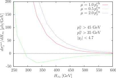
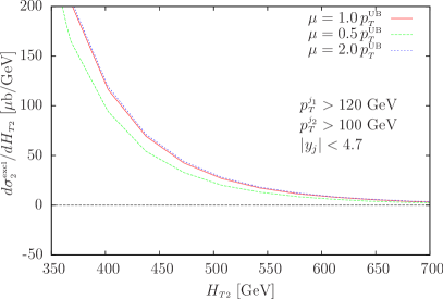
In the left plot of fig. 9, we plotted $\tilde{\sigma}_{2}^{\mathchoice{\displaystyle}{\scriptstyle}{\scriptscriptstyle}{\scriptscriptstyle}\rm excl}$, and, as expected, it becomes unphysical when the scale chosen is $p_{\mathchoice{\displaystyle}{\scriptstyle}{\scriptscriptstyle}{\scriptscriptstyle}\rm T}^{\rm\mathchoice{\displaystyle}{\scriptstyle}{\scriptscriptstyle}{\scriptscriptstyle}UB}/2$ and for values of $H_{\mathchoice{\displaystyle}{\scriptstyle}{\scriptscriptstyle}{\scriptscriptstyle}T2}\gtrsim 270$ GeV. The explanation of this can be again traced back to the large logarithmic terms related to symmetric cuts and to the increase of the value of $\alpha_{\mathchoice{\displaystyle}{\scriptstyle}{\scriptscriptstyle}{\scriptscriptstyle}\rm S}$, now evaluated at a smaller scale (the rôle played by the factorization scale would be more difficult to disentangle, since it involves the behavior of the parton distribution functions too). The two-jet exclusive cross section always gets a contribution from the Born and the virtual terms, irrespective of the value of $H_{\mathchoice{\displaystyle}{\scriptstyle}{\scriptscriptstyle}{\scriptscriptstyle}T2}$, and from the part of the real-emission cross section that, at those kinematic points, is clustered into a two-jet configuration

$$\tilde{\sigma}_{2}^{\mathchoice{\displaystyle}{\scriptstyle}{\scriptscriptstyle}{\scriptscriptstyle}\rm excl}=\tilde{\sigma}_{2}^{\mathchoice{\displaystyle}{\scriptstyle}{\scriptscriptstyle}{\scriptscriptstyle}B}+\tilde{\sigma}_{2}^{\mathchoice{\displaystyle}{\scriptstyle}{\scriptscriptstyle}{\scriptscriptstyle}V}+\tilde{\sigma}_{2}^{\mathchoice{\displaystyle}{\scriptstyle}{\scriptscriptstyle}{\scriptscriptstyle}R}=\alpha_{\mathchoice{\displaystyle}{\scriptstyle}{\scriptscriptstyle}{\scriptscriptstyle}\rm S}^{2}(\mu)\big{\{}B+\alpha_{\mathchoice{\displaystyle}{\scriptstyle}{\scriptscriptstyle}{\scriptscriptstyle}\rm S}(\mu)\big{[}V+R_{2}\big{]}\big{\}}\,,$$ (9)

where the notation is self-explanatory and we put in evidence the appearance of the strong coupling constant $\alpha_{\mathchoice{\displaystyle}{\scriptstyle}{\scriptscriptstyle}{\scriptscriptstyle}\rm S}(\mu)$ evaluated at the scale $\mu$. Since $B$ and $R_{2}$ are necessarily positive, coming from the square of the respective matrix element, it is the virtual term $V$ that drives $\tilde{\sigma}_{2}^{\mathchoice{\displaystyle}{\scriptstyle}{\scriptscriptstyle}{\scriptscriptstyle}\rm excl}$ to negative values. In other words, the $R_{2}$ term becomes smaller and smaller if compared to the absolute value of $V$. At high values of $H_{\mathchoice{\displaystyle}{\scriptstyle}{\scriptscriptstyle}{\scriptscriptstyle}T2}$ , most of the events have three jets, with the two hard jets with $p_{\mathchoice{\displaystyle}{\scriptstyle}{\scriptscriptstyle}{\scriptscriptstyle}\rm T}\sim H_{\mathchoice{\displaystyle}{\scriptstyle}{\scriptscriptstyle}{\scriptscriptstyle}T2}/2$, because, most likely, the transverse momentum of the third jet is just high enough to pass the cuts in eq. (3). Since the minimum $p_{\mathchoice{\displaystyle}{\scriptstyle}{\scriptscriptstyle}{\scriptscriptstyle}\rm T}$ for the jets is 35 GeV, the imbalance between the two hardest jets is small, and the situation is equivalent to imposing symmetric cuts. On the other hand, if we increase to 100 GeV the minimum transverse momentum to define a jet, as in the right plot of fig. 9, the imbalance between the two hardest jets is no longer small compared to their average transverse momentum, and the event kinematics stays away from the symmetric-cut configuration. In addition, we have explicitly checked that, by keeping the $p_{\mathchoice{\displaystyle}{\scriptstyle}{\scriptscriptstyle}{\scriptscriptstyle}\rm T}$ cuts of eq. (3) but restricting the jet-rapidity range to $|y_{j}|<2.5$, the critical $H_{\mathchoice{\displaystyle}{\scriptstyle}{\scriptscriptstyle}{\scriptscriptstyle}T2}$ value is moved to higher values, i.e. $\sim\!400$ GeV, implying that the unphysical behaviour depends on both the transverse momentum and the rapidity cuts.

References

- Fadin et al. (1975) V. S. Fadin, E. A. Kuraev, and L. N. Lipatov, Phys. Lett. B60, 50 (1975).
- Kuraev et al. (1976) E. A. Kuraev, L. N. Lipatov, and V. S. Fadin, Sov. Phys. JETP 44, 443 (1976).
- Kuraev et al. (1977) E. A. Kuraev, L. N. Lipatov, and V. S. Fadin, Sov. Phys. JETP 45, 199 (1977).
- Balitsky and Lipatov (1978) I. I. Balitsky and L. N. Lipatov, Sov. J. Nucl. Phys. 28, 822 (1978).
- Aad et al. (2011a) G. Aad et al. (ATLAS Collaboration), JHEP 1109, 053 (2011a), eprint 1107.1641.
- Aad et al. (2011b) G. Aad et al. (ATLAS Collaboration), Eur.Phys.J. C71, 1763 (2011b), eprint 1107.2092.
- Aad et al. (2011c) G. Aad et al. (ATLAS Collaboration) (2011c), eprint 1112.6297.
- Chatrchyan et al. (2011) S. Chatrchyan et al. (CMS), Phys.Lett. B702, 336 (2011), eprint 1106.0647.
- Khachatryan et al. (2011) V. Khachatryan et al. (CMS), Phys.Rev.Lett. 106, 122003 (2011), eprint 1101.5029.
- Chatrchyan et al. (2012) S. Chatrchyan et al. (CMS) (2012), eprint 1202.0704.
- Nason (2004) P. Nason, JHEP 0411, 040 (2004), eprint hep-ph/0409146.
- Frixione et al. (2007) S. Frixione, P. Nason, and C. Oleari, JHEP 0711, 070 (2007), eprint 0709.2092.
- Alioli et al. (2011) S. Alioli, K. Hamilton, P. Nason, C. Oleari, and E. Re, JHEP 1104, 081 (2011), eprint 1012.3380.
- Andersen and Smillie (2010a) J. R. Andersen and J. M. Smillie, JHEP 1001, 039 (2010a), eprint 0908.2786.
- Andersen and Smillie (2010b) J. R. Andersen and J. M. Smillie, Phys.Rev. D81, 114021 (2010b), eprint 0910.5113.
- Andersen and Smillie (2011) J. R. Andersen and J. M. Smillie, JHEP 1106, 010 (2011), eprint 1101.5394.
- Alioli et al. (2010) S. Alioli, P. Nason, C. Oleari, and E. Re, JHEP 1006, 043 (2010), eprint 1002.2581.
- Sjostrand et al. (2006) T. Sjostrand, S. Mrenna, and P. Z. Skands, JHEP 0605, 026 (2006), eprint hep-ph/0603175.
- Alwall et al. (2007) J. Alwall et al., JHEP 09, 028 (2007), eprint 0706.2334.
- Dokshitzer et al. (1992) Y. L. Dokshitzer, V. A. Khoze, and T. Sjostrand, Phys. Lett. B274, 116 (1992).
- Del Duca et al. (2001a) V. Del Duca, W. Kilgore, C. Oleari, C. Schmidt, and D. Zeppenfeld, Phys. Rev. Lett. 87, 122001 (2001a), eprint hep-ph/0105129.
- Del Duca et al. (2001b) V. Del Duca, W. Kilgore, C. Oleari, C. Schmidt, and D. Zeppenfeld, Nucl. Phys. B616, 367 (2001b), eprint hep-ph/0108030.
- Del Duca et al. (2004) V. Del Duca, A. Frizzo, and F. Maltoni, JHEP 05, 064 (2004), eprint hep-ph/0404013.
- Del Duca et al. (2006) V. Del Duca et al., JHEP 10, 016 (2006), eprint hep-ph/0608158.
- Campbell et al. (2006) J. M. Campbell, R. K. Ellis, and G. Zanderighi, JHEP 10, 028 (2006), eprint hep-ph/0608194.
- Campbell et al. (2010) J. M. Campbell, R. Ellis, and C. Williams, Phys.Rev. D81, 074023 (2010), eprint 1001.4495.
- Andersen et al. (2010a) J. R. Andersen et al. (SM and NLO Multileg Working Group) (2010a), eprint 1003.1241.
- Del Duca et al. (2003) V. Del Duca, W. Kilgore, C. Oleari, C. R. Schmidt, and D. Zeppenfeld, Phys. Rev. D67, 073003 (2003), eprint hep-ph/0301013.
- Andersen and White (2008) J. R. Andersen and C. D. White, Phys. Rev. D78, 051501 (2008), eprint 0802.2858.
- Andersen et al. (2009) J. R. Andersen, V. Del Duca, and C. D. White, JHEP 02, 015 (2009), eprint 0808.3696.
- Andersen et al. (2010b) J. R. Andersen, K. Arnold, and D. Zeppenfeld, JHEP 06, 091 (2010b), eprint 1001.3822.
- Forshaw et al. (2009) J. Forshaw, J. Keates, and S. Marzani, JHEP 0907, 023 (2009), eprint 0905.1350.
- Schofield and Seymour (2012) A. Schofield and M. H. Seymour, JHEP 1201, 078 (2012), 18 pages, 11 figures, eprint 1103.4811.
- Delgado et al. (2011) R. M. D. Delgado, J. R. Forshaw, S. Marzani, and M. H. Seymour, JHEP 1108, 157 (2011), eprint 1107.2084.
- Frixione and Ridolfi (1997) S. Frixione and G. Ridolfi, Nucl. Phys. B507, 315 (1997), eprint hep-ph/9707345.
- Andersen et al. (2001) J. R. Andersen, V. Del Duca, S. Frixione, C. R. Schmidt, and W. J. Stirling, JHEP 02, 007 (2001), eprint hep-ph/0101180.
- Banfi and Dasgupta (2004) A. Banfi and M. Dasgupta, JHEP 01, 027 (2004), eprint hep-ph/0312108.
- Cacciari et al. (2008) M. Cacciari, G. P. Salam, and G. Soyez, JHEP 0804, 063 (2008), eprint 0802.1189.
- Andersen et al. (2011) J. R. Andersen, L. Lönnblad, and J. M. Smillie, JHEP 1107, 110 (2011), eprint 1104.1316.
- Klasen and Kramer (1996) M. Klasen and G. Kramer, Phys.Lett. B366, 385 (1996), eprint hep-ph/9508337.
- Martin et al. (2009) A. D. Martin, W. J. Stirling, R. S. Thorne, and G. Watt, Eur. Phys. J. C63, 189 (2009), eprint 0901.0002.
- d’Enterria (2009) D. d’Enterria (2009), eprint 0911.1273.
- Orr and Stirling (1997) L. H. Orr and W. J. Stirling, Phys. Rev. D56, 5875 (1997), eprint hep-ph/9706529.
- Colferai et al. (2010) D. Colferai, F. Schwennsen, L. Szymanowski, and S. Wallon, JHEP 1012, 026 (2010), eprint 1002.1365.