Fast joint detection-estimation of evoked brain activity in event-related fMRI using a variational approach

Abstract

In standard clinical within-subject analyses of event-related fMRI data, two steps are usually performed separately: detection of brain activity and estimation of the hemodynamic response. Because these two steps are inherently linked, we adopt the so-called region-based Joint Detection-Estimation (JDE) framework that addresses this joint issue using a multivariate inference for detection and estimation. JDE is built by making use of a regional bilinear generative model of the BOLD response and constraining the parameter estimation by physiological priors using temporal and spatial information in a Markovian modeling. In contrast to previous works that use Markov Chain Monte Carlo (MCMC) techniques to approximate the resulting intractable posterior distribution, we recast the JDE into a missing data framework and derive a Variational Expectation-Maximization (VEM) algorithm for its inference. A variational approximation is used to approximate the Markovian model in the unsupervised spatially adaptive JDE inference, which allows fine automatic tuning of spatial regularisation parameters. It follows a new algorithm that exhibits interesting properties compared to the previously used MCMC-based approach. Experiments on artificial and real data show that VEM-JDE is robust to model mis-specification and provides computational gain while maintaining good performance in terms of activation detection and hemodynamic shape recovery.

I Introduction

Functional Magnetic Resonance Imaging (fMRI) is a powerful tool to non-invasively study the relationship between a sensory or cognitive task and the ensuing evoked neural activity through the neurovascular coupling measured by the BOLD signal [1]. Since the 90’s, this modality has become widely used in neuroimaging. Functional connectivity analyses aim at studying the interactions between signals and thus provide insight on integrative cerebral phenomena. In a complementary manner, we focus on the recovery of localization and dynamics of local evoked activity, thus on specialized cerebral processes. In this setting, the key issue is the modeling of the link between stimulation events and the induced BOLD effect throughout the brain. Physiological non-linear models [2, 3] are the most specific approaches to properly describe this link but their computational cost and their identifiability issues limit their use to a limited number of specific regions and to a few experimental conditions. The common approach, being the context of this paper, rather consists of linear systems which appear more robust and tractable. Here, the link between stimulation and BOLD effect is modelled through a convolutive system where each stimulus event induces a BOLD response, via the convolution of the binary stimulus sequence with the Hemodynamic Response Function (HRF). It follows two tasks for such BOLD analysis: the detection of where cerebral activity occurs and the estimation of its dynamics through the HRF identification. Commonly, the estimation part is ignored and the HRF is fixed to a canonical version which has been fitted on visual areas [4]. The detection task is performed by a General Linear Model (GLM), where stimulus-induced components are assumed to be known and only their relative weighting are to be recovered in the form of effect maps [5]. However, spatial intra-subject and between-subject variability of the response function has been highlighted [6, 7], in addition to potential timing fluctuations induced by the paradigm (eg variations in delay). To take this variability into account, more flexibility can be injected in the GLM framework by adding more regressors. In a parametric setting, this amounts to adding a function basis, such as canonical HRF derivatives or a set of gamma functions. In a non-parametric setting, all HRF coefficients are explicitely encoded as a Finite Impulse Response [8]. The major drawback of these GLM extensions is the multiplicity of regressors for a given condition, so that the detection task is more difficult to perform and that statistical power is decreased. Moreover, the more coefficients to recover, the more ill-posed the problem becomes. The alternative approaches which aim at keeping a single regressor per condition and add also a temporal regularisation constraint to fix the ill-posedness are the so-called regularized FIR methods [9, 10]. Still, they do not overcome the low signal-to-noise ratio inherent to BOLD signals, and they lack robustness especially in non-activating regions. All the issues encountered in the previously mentioned approaches are linked to the sequential treatment of the detection and estimation tasks. Indeed, these two problems are strongly linked: on the one hand, a precise localization of brain activated areas strongly depends on a reliable HRF model; on the other hand, a robust estimation of the HRF is only possible in activated areas where enough relevant signal is measured [11]. This consideration led to jointly perform these two tasks [12, 13] in a Joint Detection-Estimation (JDE) framework [14, 15] which is the basis of the approach developed in this paper. To improve the estimation robustness, a gain in HRF reproducibility is performed by spatially aggregating signals so that a constant HRF shape is locally considered across a small group of voxels, i.e. a region or a parcel. The procedure then implies a partitioning of the data into functionally homogeneous parcels, in the form of a cerebral parcellation. In brief, the JDE approach mainly rests upon: i) a non-parametric or FIR modeling of the HRF at this parcel-level for an unconstrained HRF shape; ii) prior information about the temporal smoothness of the HRF to guarantee a physiologically plausible shape; and iii) the modeling of spatial correlation between neighboring voxels within each parcel using condition-specific discrete hidden Markov fields. In [16, 15], posterior inference is carried out in a Bayesian setting using a Markov Chain Monte Carlo (MCMC) method, which is computationally intensive and requires the fine tuning of several parameters.

In this paper, we reformulate the complete JDE framework [15] as a missing data problem and propose a simplification of its estimation procedure. We resort to a variational approximation using a Variational Expectation Maximization (VEM) algorithm in order to derive estimates of the HRF and stimulus-related activity. Variational approximations have been widely and successfully employed in the context of fMRI analysis: to model auto-regressive noise in the context of a Bayesian GLM [17], to characterize cerebral hierarchical dynamic models [18], to model transient neuronal signals in a Bayesian dynamical system [14], or to perform inference of spatial mixture models for the segmentation of GLM effects maps [19]. As in our study, the primary objective of resorting to variational approximations is to alleviate the computational burden associated with stochastic MCMC approaches. Akin to [19], we aim at comparing the stochastic and variational based inference schemes but on the more complex matter of detecting activation and estimating the HRF whereas [19] treated only a detection (or segmentation) problem.

Compared to a JDE MCMC implementation, the proposed approach does not require priors on the model parameters for inference to be carried out. However, for more robustness and to make the proposed approach completely auto-calibrated, the adopted model may be extended by injecting additional priors on some of its parameters.

Experiments on artificial and real data demonstrate the good performance of our VEM algorithm. Compared to the MCMC implementation, VEM is more computationally efficient, is robust to mis-specification of the parameters, to deviations from the model and adaptable to various experimental conditions. This increases considerably the potential impact of the JDE framework and makes its application to fMRI studies in neuroscience easier and more valuable. This new framework has also the advantage of providing straightforward criteria for model selection.

The rest of this paper is organized as follows. In Section II, we introduce the hierarchical Bayesian model for the JDE framework in the within-subject fMRI context. In Section III, the VEM algorithm based on variational approximations for inference is described. Evaluation on real and artificial fMRI datasets are reported in Section IV and the performance comparison between the MCMC and VEM implementations is reported in Section V. Finally, Section VI concludes with a discussion of the points highlighted by the approach and areas for further research.

II Bayesian framework for the joint detection-estimation

Matrices and vectors are denoted with bold upper and lower case letters (e.g. $\mathb{P}$ and ${\boldsymbol{\mu}}$). A vector is by convention a column vector. The transpose is denoted by ^t. Unless stated otherwise, subscripts $j$, $m$, $i$ and $n$ are respectively indexes over voxels, stimulus types, mixture components and time point. The Gaussian distribution with mean ${\boldsymbol{\mu}}$ and covariance matrix ${\boldsymbol{\Sigma}}$ is denoted by ${\mathcal{N}}({\boldsymbol{\mu}},{\boldsymbol{\Sigma}})$.

II-A The parcel-based model

We first recast the parcel-based JDE model of [16, 15] in a missing data framework. Let us assume that the brain is decomposed in ${\boldsymbol{\mathcal{P}}}=({\mathcal{P}}_{\gamma})_{\gamma=1:\Gamma}$ parcels, each of them having homogeneous hemodynamic properties. The fMRI time series ${\mathb{y}}_{j}$ is measured in voxel $j\in{\mathcal{P}}_{\gamma}$ at times $(t_{n})_{n=1\ldots N}$, where $t_{n}=n\mathit{TR}$, $N$ being the number of scans and $\mathit{TR}$, the time of repetition. The number of different stimulus types or experimental conditions is $M$. For a given parcel ${\mathcal{P}}_{\gamma}$ containing a group of connected voxels, a unique BOLD signal model is used in order to link the observed data ${\mathb{Y}}=\{{\mathb{y}}_{j}\in\mathbb{R}^{N},j\in{\mathcal{P}}_{\gamma}\}$ to the HRF ${\mathb{h}}_{\gamma}\in\mathbb{R}^{D+1}$ specific to ${\mathcal{P}}_{\gamma}$ and to the response amplitudes ${\mathb{A}}=\{{\mathb{a}}^{m},m=1\ldots M\}$ with ${\mathb{a}}^{m}=\{a^{m}_{j},j\in{\mathcal{P}}_{\gamma}\}$ and $a_{j}^{m}$ being the magnitude at voxel $j$ for condition $m$. More specifically, the observation model at each voxel $j\in{\mathcal{P}}_{\gamma}$ is expressed as follows [16]:

$${\mathb{y}}_{j} ={\mathb{S}}_{j}{\mathb{h}}_{\gamma}+{\mathb{P}}\boldsymbol{\ell}_{j}+{\boldsymbol{\varepsilon}}_{j},\quad\text{with}\quad{\mathb{S}}_{j}=\sum_{m=1}^{M}a_{j}^{m}{\mathb{X}}_{m}$$ (1)

where ${\mathb{S}}_{j}{\mathb{h}}_{\gamma}$ is the summation of the stimulus-induced components of the BOLD signal. The binary matrix ${\mathb{X}}_{m}=\{x^{n-d\Delta t}_{m},n=1\ldots N,d=0\ldots D\}$ is of size $N\times(D+1)$ and provides information on the stimulus occurrences for the $m$-th experimental condition, $\Delta t<TR$ being the sampling period of the unknown HRF ${\mathb{h}}_{\gamma}=\{h_{d\Delta t},d=0\ldots D\}$ in ${\mathcal{P}}_{\gamma}$. This hemodynamic response is a consequence of the neuronal excitation which is commonly assumed to occur following stimulation. The scalars $a_{j}^{m}$’s are weights that model the transition between stimulations whose occurrences are informed by the ${\mathb{X}}_{m}$ matrices ($m=0\ldots M$), and the vascular response informed by the filter ${\mathb{h}}_{\gamma}$. It follows that the $a_{j}^{m}$’s are generally referred to as Neural Response Levels (NRL). The rest of the signal is made of matrix ${\mathb{P}}$, which corresponds to physiological artifacts accounted for via a low frequency orthonormal function basis of size $N\times O$. At each voxel $j$ is associated a vector of low frequency drifts $\boldsymbol{\ell}_{j}\in\mathbb{R}^{O}$ which has to be estimated. Within parcel ${\mathcal{P}}_{\gamma}$, these vectors may be grouped into the same matrix ${\mathb{L}}=\{\boldsymbol{\ell}_{j},j\in{\mathcal{P}}_{\gamma}\}$. Regarding the observation noise, the ${\boldsymbol{\varepsilon}}_{j}$’s are assumed to be independent with ${\boldsymbol{\varepsilon}}_{j}\sim{\mathcal{N}}(0,{\boldsymbol{\Gamma}}_{j}^{-1})$ at voxel $j$ (see Section II-B1 for more details). The set of all unknown precision matrices (inverse of the covariance matrices) is denoted by ${\boldsymbol{\Gamma}}=\left\{{\boldsymbol{\Gamma}}_{j},j\in{\mathcal{P}}_{\gamma}\right\}$.

Finally, detection is handled through the introduction of activation class assignments ${\mathb{Q}}=\bigl{\{}{\mathb{q}}^{m},m=1\ldots M\bigr{\}}$ where ${\mathb{q}}^{m}=\bigl{\{}q_{j}^{m},j\in{\mathcal{P}}_{\gamma}\bigr{\}}$ and $q_{j}^{m}$ represents the activation class at voxel $j$ for experimental condition $m$. The NRL coefficients will therefore be expressed conditionally to these hidden variables. In other words, the NRL coefficients will depend on the activation status of the voxel $j$, which itself depends on the activation status of neighbouring voxels thanks to a Markov model used as a spatial prior on ${\mathb{Q}}$ (cf Section II-B2). Without loss of generality, here the number of classes is $I=2$ for activated and non-activated voxels. An additional deactivation class ($I=3$) may be considered depending on the experiment. In the following developments, all provided formulas are general enough to cover this case.

II-B A hierarchical Bayesian Model

In a Bayesian framework, we first need to define the likelihood and prior distributions for the model variables $({\mathb{Y}},{\mathb{A}},{\mathb{h}}_{\gamma},{\mathb{Q}})$ and parameters $({\boldsymbol{\Theta}})$. Using the hierarchical structure between ${\mathb{Y}}$, ${\mathb{A}}$, ${\mathb{h}}_{\gamma}$, ${\mathb{Q}}$ and ${\boldsymbol{\Theta}}$, the complete model is given by the joint distribution of both the observed and unobserved (or missing) data: $p({\mathb{Y}},{\mathb{A}},{\mathb{h}}_{\gamma},{\mathb{Q}};{\boldsymbol{\Theta}})=p({\mathb{Y}}\,|\,{\mathb{A}},{\mathb{h}}_{\gamma};{\boldsymbol{\Theta}})\;\;p({\mathb{h}}_{\gamma};{\boldsymbol{\Theta}})p({\mathb{A}}\,|\,{\mathb{Q}};{\boldsymbol{\Theta}})\;p({\mathb{Q}};{\boldsymbol{\Theta}}).$ To fully define the hierarchical model, we now specify each term in turn.

II-B1 Likelihood

The definition of the likelihood depends on the noise model. In [20, 21], an autoregressive (AR) noise model has been adopted to account for serial correlations in fMRI time series. It has also been shown in [21] that a spatially-varying first-order AR noise model helped controlling false positive rate. In the same context, we will assume such a noise model ${\boldsymbol{\varepsilon}}_{j}\sim{\mathcal{N}}({\mathbf{0}},{\boldsymbol{\Gamma}}_{j}^{-1})$ with ${\boldsymbol{\Gamma}}_{j}=\sigma_{j}^{-2}{\boldsymbol{\Lambda}}_{j}$ where ${\boldsymbol{\Lambda}}_{j}$ is a tridiagonal symmetric matrix which depends on the AR(1) parameter $\rho_{j}$ [16]: $({\boldsymbol{\Lambda}}_{j})_{1,1}=({\boldsymbol{\Lambda}}_{j})_{N,N}=1$, $({\boldsymbol{\Lambda}}_{j})_{n,n}=1+\rho_{j}^{2}$ for $n=2:N-1$ and $({\boldsymbol{\Lambda}}_{j})_{n+1,n}=({\boldsymbol{\Lambda}}_{j})_{n,n+1}=-\rho_{j}$ for $n=1:N-1$. These parameters are assumed voxel-varying due to their tissue-dependence [22, 23]. The likelihood can therefore be decomposed as:

$$p({\mathb{Y}}\,|\,{\mathb{A}},{\mathb{h}}_{\gamma};{\mathb{L}},{\boldsymbol{\Gamma}}) \propto\prod_{j\in{\mathcal{P}}_{\gamma}}|{\boldsymbol{\Gamma}}_{j}|^{{-1/2}}\exp\bigl{(}-\frac{1}{2}\overline{{\mathb{y}}}_{j}^{\mathrm{t}}{\boldsymbol{\Gamma}}_{j}\overline{{\mathb{y}}}_{j}\bigr{)},$$ (2)

where $|{\boldsymbol{\Gamma}}_{j}|=\sigma_{j}^{-2N}\,|{\boldsymbol{\Lambda}}_{j}|$, $|{\boldsymbol{\Lambda}}_{j}|=1-\rho_{j}^{2}$ and $\overline{{\mathb{y}}}_{j}={\mathb{y}}_{j}-{\mathb{P}}\boldsymbol{\ell}_{j}-{\mathb{S}}_{j}{\mathb{h}}_{\gamma}$.

II-B2 Model priors

HRF

Akin to [16, 15], we introduce constraints in the HRF prior that favor smooth variations in ${\mathb{h}}_{\gamma}$ by controlling its second order derivative: ${\mathb{h}}_{\gamma}\sim{\mathcal{N}}(0,v_{\mathb{h}}{\mathb{R}})\;\text{with\>}{\mathb{R}}=(\Delta t)^{4}\;({\mathb{D}}_{2}^{\mathrm{t}}{\mathb{D}}_{2})^{-1}$ where ${\mathb{D}}_{2}$ is the second-order finite difference matrix and $v_{\mathb{h}}$ is a parameter to be estimated. Moreover, boundary constraints have also been fixed on ${\mathb{h}}_{\gamma}$ as in [16, 15] so that $h_{0}=h_{D\Delta t}=0$.

Neuronal response levels

Akin to [16, 15], the NRLs $a_{j}^{m}$ are assumed to be statistically independent across conditions: $p({\mathb{A}};{\boldsymbol{\theta}}_{{\mathb{a}}})=\prod\limits_{m}p({\mathb{a}}^{m};{\boldsymbol{\theta}}_{m})$ where ${\boldsymbol{\theta}}_{{\mathb{a}}}=\{{\boldsymbol{\theta}}_{m},m=1\ldots M\}$ and ${\boldsymbol{\theta}}_{m}$ gathers the parameters for the $m$-th condition. A mixture model is then adopted by using the assignment variables $q_{j}^{m}$ to segregate non-activated voxels ($q_{j}^{m}=1$) from activated ones ($q_{j}^{m}=2$). For the $m$-th condition, and conditionally to the assignment variables ${\mathb{q}}^{m}$, the NRLs are assumed to be independent: $p({\mathb{a}}^{m}\,|\,{\mathb{q}}^{m};{\boldsymbol{\theta}}_{m})=\prod\limits_{j\in{\mathcal{P}}_{\gamma}}p(a_{j}^{m}\,|\,q_{j}^{m};{\boldsymbol{\theta}}_{m})$. If $q_{j}^{m}=i$ then $p(a_{j}^{m}\,|\,q_{j}^{m}=i;{\boldsymbol{\theta}}_{m})\sim{\mathcal{N}}(\mu_{im},v_{im})$. The Gaussian parameters ${\boldsymbol{\theta}}_{m}=\{\mu_{im},v_{im},i=1\ldots I\}$ are unknown. We denote by ${\boldsymbol{\mu}}\!=\!\!\{{\boldsymbol{\mu}}_{m},m=1\ldots M\}$ with ${\boldsymbol{\mu}}_{m}=\{\mu_{1m},\ldots,\mu_{Im}\}$ and ${\mathb{v}}=\{{\mathb{v}}_{m},m=1\ldots M\}$ with ${\mathb{v}}_{m}=\{v_{1m},\ldots,v_{Im}\}$. More specifically, for non-activating voxels we set for all $m$, $\mu_{1m}\!=\!0$.

Activation classes

As in [15], we assume prior independence between the $M$ experimental conditions regarding the activation class assignments. It follows that $p({\mathb{Q}})\!=\!\prod\limits_{m=1}^{M}p({\mathb{q}}^{m};\beta_{m})$ where we assume in addition that $p({\mathb{q}}^{m};\beta_{m})$ is a spatial Markov prior, namely a Potts model with interaction parameter $\beta_{m}$ [15]:

$$p({\mathb{q}}^{m};\beta_{m}) =Z(\beta_{m})^{-1}\exp\bigl{(}\beta_{m}U({\mathb{q}}^{m})\bigr{)}\quad\text{with}\quad U({\mathb{q}}^{m})=\sum_{{j\thicksim k}}{\delta(q_{j}^{m},q_{k}^{m})}$$ (3)

and where $Z(\beta_{m})$ is the normalizing constant and for all $(a,b)\in\mathbb{R}^{2}\;,\;{\delta(a,b)}=1$ if $a=b$ and 0 otherwise. The notation $j\thicksim k$ means that the summation is over all neighboring voxels. Moreover, the neighboring system may cover a 3D scheme through the brain volume. The unknown parameters are denoted by ${\boldsymbol{\beta}}=\left\{\beta_{m},m=1\ldots M\right\}$. In what follows, we will consider a 6-connexity 3D neighboring system.

For the complete model, the whole set of parameters is denoted by ${\boldsymbol{\Theta}}=\left\{{\boldsymbol{\Gamma}},{\mathb{L}},{\boldsymbol{\mu}},{\mathb{v}},{\mathb{v}}_{h},{\boldsymbol{\beta}}\right\}$ and belong to a set $\underline{{\boldsymbol{\Theta}}}$.

III Estimation by variational Expectation-Maximization

We propose to use an Expectation-Maximization (EM) framework to deal with the missing data namely, ${\mathb{A}}\in\mathcal{A}$, ${\mathb{h}}_{\gamma}\in\mathcal{H}$, ${\mathb{Q}}\in\mathcal{Q}$. Let $\mathcal{D}$ be the set of all probability distributions on $\mathcal{A}\times\mathcal{H}\times\mathcal{Q}$. EM can be viewed [24] as an alternating maximization procedure of a function ${\mathcal{F}}$ on $\mathcal{D}$, ${\mathcal{F}}(p,{\boldsymbol{\Theta}})={\mathrm{E}}_{p}\bigl{[}\log p({\mathb{Y}},{\mathb{A}},{\mathb{h}}_{\gamma},{\mathb{Q}}\,|\,{\boldsymbol{\Theta}})\bigr{]}+{\mathcal{G}}(p)$ where ${\mathrm{E}}_{p}\bigl{[}.\bigr{]}$ denotes the expectation with respect to $p$ and ${\mathcal{G}}(p)=-{\mathrm{E}}_{p}\bigl{[}\log p({\mathb{A}},{\mathb{h}}_{\gamma},{\mathb{Q}})\bigr{]}$ is the entropy of $p$. At iteration $(r)$, denoting the current parameter values by ${\boldsymbol{\Theta}}^{(r-1)}$, the alternating procedure proceeds as follows:

E-step: $$p^{(r)}_{A,H_{\gamma},Q}=\mathop{\mathrm{arg\,max}}\limits_{p\in\mathcal{D}}\;{\mathcal{F}}(p,{\boldsymbol{\Theta}}^{(r-1)})$$ (4)

M-step: $${\boldsymbol{\Theta}}^{(r)}=\mathop{\mathrm{arg\,max}}\limits_{\Theta\in\underline{{\boldsymbol{\Theta}}}}\;{\mathcal{F}}(p^{(r)}_{A,H_{\gamma},Q},{\boldsymbol{\Theta}})$$ (5)

The optimization step in Eq. (4) leads to $p^{(r)}_{A,H_{\gamma},Q}=p({\mathb{A}},{\mathb{h}}_{\gamma},{\mathb{Q}}\,|\,{\mathb{Y}},{\boldsymbol{\Theta}}^{(r-1)})$, which is intractable for our model. Hence, we resort to a variational EM variant in which the intractable posterior is approximated as a product of three pdfs on $\mathcal{A}$, $\mathcal{H}$ and $\mathcal{Q}$ respectively.

Previous attempts to use variational inference [25] in fMRI [19, 17] have been successful with this type of approximations usually validated by assessing its fidelity to its MCMC counterpart. In Section IV, we will also provide such a comparison. The fact that the HRF ${\mathb{h}}_{\gamma}$ can be equivalently considered as missing variables or random parameters induces some similarity between our Variational EM variant and the Variational Bayesian EM algorithm presented in [25]. Our framework varies slightly from the case of conjugate exponential models described in [25] and more importantly, our presentation offers the possibility to deal with extra parameters ${\boldsymbol{\Theta}}$ for which prior information may not be available.
We propose here to use an EM variant in which the intractable E-step is instead solved over $\tilde{{\mathcal{D}}}$, a restricted class of probability distributions chosen as the set of distributions that factorize as $\widetilde{p}_{A,H_{\gamma},Q}=\widetilde{p}_{A}\widetilde{p}_{H_{\gamma}}\widetilde{p}_{Q}$ where $\widetilde{p}_{A}$, $\widetilde{p}_{H_{\gamma}}$ and $\widetilde{p}_{Q}$ are probability distributions on $\mathcal{A}$, $\mathcal{H}$ and $\mathcal{Q}$, respectively. It follows then that our E-step becomes an approximate E-step, which can be further decomposed into three stages that consist of updating the three pdfs, $\widetilde{p}_{H_{\gamma}}$, $\widetilde{p}_{A}$ and $\widetilde{p}_{Q}$, in turn using three equivalent expressions of ${\mathcal{F}}$ when $p$ factorizes as in $\tilde{\mathcal{D}}$. At iteration $(r)$ with current estimates denoted by $\widetilde{p}_{H}^{(r-1)},\widetilde{p}_{A}^{(r-1)},\widetilde{p}_{Q}^{(r-1)}$ and ${\boldsymbol{\Theta}}^{(r-1)}$, the updating rules become:

$$\text{{\bf E-H:} }\;\widetilde{p}_{H_{\gamma}}^{(r)} =\mathop{\mathrm{arg\,max}}_{p_{H_{\gamma}}}{\mathcal{F}}(\widetilde{p}_{A}^{(r-1)}\;p_{H_{\gamma}}\;\widetilde{p}_{Q}^{(r-1)},{\boldsymbol{\Theta}}^{(r-1)})$$

$$\text{{\bf E-A:} }\;\widetilde{p}_{A}^{(r)} =\mathop{\mathrm{arg\,max}}_{p_{A}}{\mathcal{F}}(p_{A}\;\widetilde{p}_{H_{\gamma}}^{(r)}\;\widetilde{p}_{Q}^{(r-1)},{\boldsymbol{\Theta}}^{(r-1)})$$

$$\text{{\bf E-Q:} }\;\widetilde{p}_{Q}^{(r)} =\mathop{\mathrm{arg\,max}}_{p_{Q}}{\mathcal{F}}(\widetilde{p}_{A}^{(r)}\;\widetilde{p}_{H_{\gamma}}^{(r)}\;p_{Q},{\boldsymbol{\Theta}}^{(r-1)}).$$

Introducing the Kullback-Leibler divergence between $\widetilde{p}_{A,H_{\gamma},Q}$ and $p_{A,H_{\gamma},Q}$ , we have

$${\mathcal{D}}(\widetilde{p}_{A,H_{\gamma},Q}\,||\,p_{A,H_{\gamma},Q}) =\int\widetilde{p}_{A,H_{\gamma},Q}({\mathb{A}},{\mathb{h}}_{\gamma},{\mathb{Q}})\log\frac{\widetilde{p}_{A,H_{\gamma},Q}({\mathb{A}},{\mathb{h}}_{\gamma},{\mathb{Q}})}{p_{A,H_{\gamma},Q}({\mathb{A}},{\mathb{h}}_{\gamma},{\mathb{Q}})}\,d{\mathb{A}}\,d{\mathb{h}}_{\gamma}\,d{\mathb{Q}}.$$ (6)

According to [24], we also have ${\mathcal{F}}(\widetilde{p}_{A,H_{\gamma},Q},{\boldsymbol{\Theta}})=\log p({\mathb{Y}};{\boldsymbol{\Theta}})-{\mathcal{D}}(\widetilde{p}_{A,H_{\gamma},Q}\,||\,p_{A,H_{\gamma},Q})$ so that the steps above can be equivalently written in terms of minimizations of the Kullback-Leibler divergence. The properties of the latter lead to the following solutions:

$$\text{{\bf E-H:} }\;\widetilde{p}_{H_{\gamma}}^{(r)}({\mathb{h}}_{\gamma}) \propto\exp\left({\mathrm{E}}_{\widetilde{p}_{A}^{(r-1)}\widetilde{p}_{Q}^{(r-1)}}\bigl{[}\log p({\mathb{h}}_{\gamma}\,|\,{\mathb{Y}},{\mathb{A}},{\mathb{Q}};{\boldsymbol{\Theta}}^{(r-1)}\bigr{]}\right)$$ (7)

$$\text{{\bf E-A:} }\;\widetilde{p}_{A}^{(r)}({\mathb{A}}) \propto\exp\left({\mathrm{E}}_{\widetilde{p}_{H_{\gamma}}^{(r)}\widetilde{p}_{Q}^{(r-1)}}\bigl{[}\log p({\mathb{A}}\,|\,{\mathb{Y}},{\mathb{h}}_{\gamma},{\mathb{Q}};{\boldsymbol{\Theta}}^{(r-1)})\bigr{]}\right)$$ (8)

$$\text{{\bf E-Q:} }\;\widetilde{p}_{Q}^{(r)}({\mathb{Q}}) \propto\exp\left({\mathrm{E}}_{\widetilde{p}_{A}^{(r)}\widetilde{p}_{H_{\gamma}}^{(r)}}\bigl{[}\log p({\mathb{Q}}\,|\,{\mathb{Y}},{\mathb{A}},{\mathb{h}}_{\gamma};{\boldsymbol{\Theta}}^{(r-1)})\bigr{]}\right)\;.$$ (9)

The corresponding M-step is (since ${\boldsymbol{\Theta}}$ and ${\mathcal{G}}(p^{(r)}_{A,H_{\gamma},Q})$ are independent):

$$\qquad\text{{\bf M:} }\;{\boldsymbol{\Theta}}^{(r)} =\mathop{\mathrm{arg\,max}}_{{\boldsymbol{\Theta}}}\;{\mathrm{E}}_{\widetilde{p}_{A}^{(r)}\widetilde{p}_{H_{\gamma}}^{(r)}\widetilde{p}_{Q}^{(r)}}\bigl{[}\log p({\mathb{Y}},{\mathb{A}},{\mathb{h}}_{\gamma},{\mathb{Q}};{\boldsymbol{\Theta}})\bigr{]}\;.$$ (10)

These steps lead to explicit calculations for $\widetilde{p}^{(r)}_{H_{\gamma}}$, $\widetilde{p}^{(r)}_{A}$, $\widetilde{p}^{(r)}_{Q}$ and the parameter set ${\boldsymbol{\Theta}}^{(r)}=\left\{{\boldsymbol{\Gamma}}^{(r)},{\mathb{L}}^{(r)},{\boldsymbol{\mu}}^{(r)},{\mathb{v}}^{(r)},{\mathb{v}}_{h}^{(r)},{\boldsymbol{\beta}}^{(r)}\right\}$.

• E-H step: From Eq. (7) standard algebra enables to derive that $\widetilde{p}^{(r)}_{H_{\gamma}}$ is a Gaussian distribution $\widetilde{p}^{(r)}_{H_{\gamma}}\sim{\mathcal{N}}({\mathb{m}}_{H_{\gamma}}^{(r)},{\boldsymbol{\Sigma}}_{H_{\gamma}}^{(r)})$ whose parameters are detailed in Appendix -A. The expressions for ${\mathb{m}}_{H_{\gamma}}^{(r)}$ and ${\boldsymbol{\Sigma}}_{H_{\gamma}}^{(r)}$ are similar to those derived in the MCMC case [16, Eq. (B.1)] with expressions involving the $a_{j}^{m}$’s replaced by their expectations wrt $\widetilde{p}_{A}^{(r-1)}$.

• E-A step : Using Eq. (8), standard algebra rules allow to identify the Gaussian distribution of $\widetilde{p}^{(r)}_{A}$ which writes as $\widetilde{p}^{(r)}_{A}=\prod_{j\in{\mathcal{P}}_{\gamma}}\widetilde{p}^{(r)}_{A_{j}}$ with $\widetilde{p}^{(r)}_{A_{j}}\sim{\mathcal{N}}({\mathb{m}}_{A_{j}}^{(r)},{\boldsymbol{\Sigma}}_{A_{j}}^{(r)})$. More detail about the update of $\widetilde{p}^{(r)}_{A}$ is given in Appendix -B. The relationship with the MCMC update of ${\mathb{A}}$ is not straightforward. In [16, 15], the $a_{j}^{m}$’s are sampled independently and conditionally on the $q_{j}^{m}$’s. This is not the case in the VEM framework but some similarity appears if we set the probabilities $\widetilde{p}^{(r-1)}_{Q_{j}^{m}}(i)$ either to 0 or 1 and consider only the diagonal part of ${\boldsymbol{\Sigma}}_{A_{j}}^{(r)}$.

• E-Q step: Using the expressions of $p({\mathb{A}}|{\mathb{Q}})$ and $p({\mathb{Q}})$ in Section II, Eq. (9) yields $\widetilde{p}^{(r)}_{Q}({\mathb{Q}})\!=\!\!\prod\limits_{m=1}^{M}\widetilde{p}^{(r)}_{Q^{m}}({\mathb{q}}^{m})$ which is intractable due to the Markov prior. To overcome this difficulty, a number of approximation techniques are available. To decrease the computational complexity of our EM algorithm or to avoid introducing additional variables as done in [19], we use a mean-field like algorithm which consists of fixing the neighbours to their mean value. Following [26], $\widetilde{p}_{Q^{m}}^{(r)}({\mathb{q}}^{m})$ can be approximated by a factorized density $\widetilde{p}_{Q^{m}}^{(r)}({\mathb{q}}^{m})=\prod\limits_{j\in{\mathcal{P}}_{\gamma}}\widetilde{p}_{Q_{j}^{m}}^{(r)}(q_{j}^{m})$ such that if $q_{j}^{m}=i$,

  $$\widetilde{p}_{Q_{j}^{m}}^{(r)}(i)\propto{\mathcal{N}}({\mathb{m}}_{A_{j}^{m}}^{(r)};\mu_{im}^{(r-1)},v_{im}^{(r-1)})f(q_{j}^{m}=i\,|\,\tilde{q}_{\sim j}^{m};\beta_{m}^{(r-1)},{\mathb{v}}_{m}^{(r-1)}),$$ (11)

  where $\tilde{{\mathb{q}}}^{m}$ is a particular configuration of ${\mathb{q}}^{m}$ updated at each iteration according to a specific scheme, $\sim j$ denotes neighbouring voxels to $j$ on the brain volume and $f(q_{j}^{m}=i\,|\,\tilde{q}_{\sim j}^{m};\beta_{m}^{(r-1)},{\mathb{v}}_{m}^{(r-1)})\propto\exp\{\frac{v_{A_{j}^{m}A_{j}^{m}}^{(r)}}{v_{im}^{(r-1)}}+\beta_{m}^{(r-1)}\sum\limits_{k\sim j}{\delta(\tilde{q}_{k}^{m},i)}\}$. Hereabove, $m_{A_{j}^{m}}^{(r)}$ and $v_{A_{j}^{m}A_{j}^{m^{\prime}}}^{(r)}$ denote the $m$ and $(m,m^{\prime})$ entries of the mean vector (${\mathb{m}}_{A_{j}}^{(r)}$) and covariance matrix (${\boldsymbol{\Sigma}}_{A_{j}}^{(r)}$), respectively. The Gaussian distribution with mean $\mu_{im}$ and variance $v_{im}$ is denoted by ${\mathcal{N}}(\;.\;;\mu_{im},v_{im})$, while $\tilde{q}_{\sim j}^{m}=\{\tilde{q}_{k}^{m},k\sim j\}$. More details are given in Appendix -C.

• M step: For this maximization step, we can first rewrite Eq. (10) as

  $${\boldsymbol{\Theta}}^{(r)} =\mathop{\mathrm{arg\,max}}_{{\boldsymbol{\Theta}}}\;\Big{[}{\mathrm{E}}_{\widetilde{p}_{A}^{(r)}\widetilde{p}_{H_{\gamma}}^{(r)}}\bigl{[}\log p({\mathb{Y}}\,|\,{\mathb{A}},{\mathb{h}}_{\gamma};{\mathb{L}},{\boldsymbol{\Gamma}})\bigr{]}+{\mathrm{E}}_{\widetilde{p}_{A}^{(r)}\widetilde{p}_{Q}^{(r)}}\bigl{[}\log p({\mathb{A}}\,|\,{\mathb{Q}};{\boldsymbol{\mu}},{\mathb{v}})\bigr{]}$$

  $$+{\mathrm{E}}_{\widetilde{p}_{H_{\gamma}}^{(r)}}\bigl{[}\log p({\mathb{h}}_{\gamma};{\mathb{v}}_{h})\bigr{]}+{\mathrm{E}}_{\widetilde{p}_{Q}^{(r)}}\bigl{[}\log p({\mathb{Q}};{\boldsymbol{\beta}})\bigr{]}\Big{]}.$$ (12)

  The M-step can therefore be decoupled into four sub-steps involving separately $({\mathb{L}},{\boldsymbol{\Gamma}})$, $({\boldsymbol{\mu}},{\mathb{v}})$, ${\mathb{v}}_{h}$ and ${\boldsymbol{\beta}}$. Some of these sub-steps admit closed-form expressions, while some other require resorting to iterative or alternate optimization. For more details about related calculations, the interested reader can refer to Appendix -D.

IV Validation of the proposed approach

This section aims at validating the proposed variational approach. Simulated and real contexts are considered respectively in sub-sections IV-A and IV-B. To corroborate the effectiveness of the proposed method, comparisons with its MCMC counterpart will also be conducted throughout the present section.

IV-A Artificial fMRI datasets

In this section, experiments have been conducted on data simulated according to the observation model in Eq. (1) where $\mathb{P}$ has been defined from a cosine transform basis as in [16]. The simulation process is illustrated in Fig 1.

${\mathb{S}}_{j}$	${\mathb{h}}_{\gamma}$	$\varepsilon_{j}$ + ${\mathb{P}}\ell_{j}$	${\mathb{y}}_{j}$
$\star$	$+$	=
scan number	Time in s	scan number	scan number

Figure 1: From left to right: ${\mathb{S}}_{j}$ represents the experimental conditions for voxel $j$ as the scan number increases. They are convoluted with the hemodynamic model ${\mathb{h}}_{\gamma}$ of parcel ${\mathcal{P}}_{\gamma}$; $\varepsilon_{j}$ + ${\mathb{P}}\ell_{j}$ represents the noise and artifact components for voxel $j$ with respect to the scan number and ${\mathb{y}}_{j}$ is the final fMRI time series simulated at voxel $j$.

Different studies have then been conducted in order to validate the detection-estimation performance and robustness. For each of these studies, some simulation parameters have been changed such as the noise or the paradigm properties. Changing these parameters aims at providing for each simulation context a realistic BOLD signal.

IV-A1 Detection-Estimation performance

Data have been simulated here with a Gaussian white noise ${\boldsymbol{\Gamma}}^{-1}_{j}=1.2~{}{\mathb{I}}_{N}$ (${\mathb{I}}_{N}$ is the $N\times N$ identity matrix). Two experimental conditions have also been considered ($M=2$) while ensuring stimulus-varying Contrast-to-Noise Ratios (CNR) achieved by setting $\mu_{12}=2.8,v_{12}=0.5^{2}$ and $\mu_{22}=1.8,v_{22}=0.5^{2}$ so that higher CNR is simulated for the first experimental condition ($m=1$) compared to the second one ($m=2$). For each of these conditions, the initial artificial paradigm comprised 30 stimulus events. The simulation process finally yielded time-series of 268 time-points. Condition-specific activating and non-activating voxels were defined as 20$\times$20 2D slices as shown in Fig. 2[left], respectively.

	Ground Truth	MCMC	VEM
$m=1$
$m=2$

Figure 2: Ground truth (left) and estimated Posterior probability maps (PPM) using MCMC (middle) and VEM (right). Condition $m=2$ (Bottom row) represents a lower CNR than condition $m=1$ (top row).

The posterior probability maps (PPM) obtained using VEM and MCMC are shown in Fig. 2[middle] and Fig. 2[right]. PPMs here correspond to the activation class assignment probability. These figures clearly show the gain in robustness provided by the variational approximation. This gain consists of lower miss-classification noise (a lower false positive rate) illustrated by higher PPM values, especially for the experimental condition with the lowest CNR ($m=2$).
For a quantitative evaluation, the ROC curves corresponding to the estimated PPMs using both algorithms were computed. They are reported in Fig. 3 and confirm that the proposed VEM approach outperforms the MCMC implementation for the second experimental condition ($m=2$). Conversely, for the higher CNR ($m=1$), the MCMC approach performs slightly better.

	$m=1$		$m=2$
sensitivity		sensitivity
	1-specificity		1-specificity

Figure 3: ROC curves associated with the label estimates using VEM and MCMC. Condition $m=1$ presents higher CNR than condition $m=2$. Curves are plotted in solid and dashed line for VEM and MCMC, respectively.

Fig. 4 shows the NRL estimates obtained by the two methods. Although some differences are exhibited on the PPM, both algorithms report similar qualitative results. However, Fig. 4[right] shows the difference between NRL estimates (VEM-MCMC). It is worth noticing in this figure that regions corresponding to activated areas for the two conditions present positive intensity values, which shows that VEM helps retrieving stronger NRL values for activated area compared to MCMC. Quantitatively speaking, the gain in robustness is confirmed by reporting the Mean Square Error (MSE) values on NRL estimates which are slightly lower using VEM compared to MCMC for the first experimental condition ($m=1$: $\rm MSE_{\rm MCMC}=0.012$ vs. $\rm MSE_{\rm VEM}=0.010$), as well as for the second experimental condition ($m=2$: $\rm MSE_{\rm MCMC}=0.010$ vs. $\rm MSE_{\rm VEM}=0.009$). These error values indicate that, even though the MCMC algorithm gives the most precise PPMs for the high CNR condition (Fig. 3, $m=1$), the VEM approach is more robust than its MCMC alternative in terms of estimated response levels. These values also indicate slightly lower MSE for the second experimental conditions ($m=2$) compared to the first one ($m=1$) with higher CNR. This difference is due to the presence of larger non-activated area used for $m=2$ where low NRL values are simulated, and for which MSE is very low.

	Ground Truth	MCMC	VEM		VEM-MCMC
$m=1$
$m=2$

Figure 4: Ground truth and NRL estimates by MCMC and VEM (first three images), and difference NRL image (right).

As regards HRF estimates, Fig. 5 shows both retrieved shapes using MCMC and VEM. Compared to the ground truth curve (solid line), the two approaches give very similar results and preserve the most important features of the original HRF like the peak value (PV), time-to-peak (TTP) and time-to-undershoot (TTU).

$\%\Delta$BOLD signal

Time (s)

Figure 5: Ground truth and estimates HRFs using the MCMC and VEM algorithms.

IV-A2 Estimation robustness

Since estimation errors may be caused by several sources of perturbation (e.g. noise level, stimulus density,…), several experiments have been conducted with different values of simulation parameters.

Varying the stimulus density

In this experiment, several simulations have been generated using different stimulus densities in the artificial paradigm (from 5 to 30 stimuli), which leads to different Inter Stimuli Intervals (ISI) (from 47 s to 9 s). Note here that the stimuli are interleaved between the two conditions so that the above-mentioned ISIs correspond to the time interval between two events irrespective to the condition they belong to. A second order autoregressive noise (AR(2)) has also been used since it has been reported in the literature that such a model provided realistic BOLD signal [21]. The rest of the model is specified as before. In order to quantitatively evaluate the robustness of the proposed VEM approach to input Signal to Noise Ratio (SNR), results (assuming white noise for both algorithms) are compared while varying the stimulation rate during the BOLD signal acquisition. Fig. 6 illustrates the MSE evolution related to the NRL estimates for both experimental conditions wrt the ISI (or equivalently the stimulus density) in the experimental paradigm. This figure shows that at low SNR level, i.e. high ISI (or low stimulus density), and for both conditions, VEM is more robust to model mispecification. In contrast, at low ISI (i.e. high stimulus density), the two methods perform similarly and remain quite robust. It should be noted here that, as reported in Section IV-A1, the error values on NRL estimates remain comparable for both experimental conditions and for all ISI values, although PPM results may present some imprecisions for the low CNR condition. Results shown in Fig. 6 were obtained over 100 simulations to investigate the NRL estimation MSE variance through runs. It can therefore be noticed through this figure that, for the two experimental conditions, higher MSE variance (larger error bars) is obtained with MCMC compared to VEM. Moreover, estimation variance across simulations (error bars) increase with ISI as expected.

	$m=1$		$m=2$
MSE		MSE
	ISI (s)		ISI (s)

Figure 6: MSE evolution of NRL estimates wrt Inter Stimuli Interval (ISI) for experimental conditions $m=1$ and $m=2$. Vertical bars represent empirical standard deviations computed over 100 simulations.

As regards hemodynamics properties, Fig. 7[left] depicts the MSE on HRF estimates inferred by the VEM and MCMC wrt the ISI (or equivalently the stimulus density). The VEM approach performs better than the MCMC one especially at low stimulus density (high ISI values), but the error level remains relatively low for both methods. When evaluating the estimation robustness of the key HRF features (PV, TTP and TTU), it turns out that the TTP and TTU estimates remain the same irrespective to the inference algorithm, which corroborates the robustness of the developed approach (results not shown). As regards PV estimates, Fig. 7[right] shows the MSE values wrt the ISI. The VEM algorithm still performs better than the MCMC one mainly at high ISI values (low stimulus density). For more complete comparisons, similar experiments have been conducted while changing the ground truth HRF properties (PV, TTP, TTU), and coherent results have been obtained.

	HRF		PV
MSE		MSE
	ISI (s)		ISI (s)

Figure 7: MSE for the HRF estimates (left) and the corresponding peak values (right) wrt interstimuli interval expressed in seconds for VEM and MCMC.

Varying the noise parameters

In this experiment, several simulations have been conducted using an AR(2) noise with different variance and correlation parameters in order to illustrate the robustness of the proposed VEM approach to noise parameter fluctuation. In Fig. 8, MSE on NRL estimates is plotted against the input SNR when varying the noise variance (Fig. 8[top]) and its amount of autocorrelation (Fig. 8[bottom]). In the latter case, the AR parameters are changed while maintaining a stable AR(2) process. As already observed in [27], at a fixed input SNR value, the impact of large autocorrelation is stronger than that of large noise variance irrespective of the inference scheme. At low input SNR (as usually observed on real BOLD signals), this feature is mainly shown through Figs. 8[bottom]-[top]. Moreover, although a slight advantage is observed for the proposed VEM approach in terms of MSE and for both experimental conditions, the two methods perform generally well with a relatively low error level. The illustrated results were obtained over 100 simulations in order to investigate the estimation error variance (vertical bars in Fig. 8). These error bars show that changing the amount of correlation (Fig. 8[top]) induces lower variance across simulations than when changing the noise variance (Fig. 8[bottom]).

	$m=1$		$m=2$
MSE		MSE
	Input SNR (dB)		Input SNR (dB)
MSE		MSE
	Input SNR (dB)		Input SNR (dB)

Figure 8: MSE evolution of NRL estimates wrt input SNR (AR(2) noise) by varying the noise variance (top row) and the amount of AR(2) noise autocorrelation (bottom row).

Varying the spatial regularisation parameter

This section is dedicated to studying the robustness of the spatial regularisation parameter estimation. When positive, this parameter favors spatial regularity across adjacent voxels, and hence smoother activation maps. Fig. 9 shows the estimated mean value and standard deviations for ${\boldsymbol{\beta}}$ over 100 simulations using both algorithms and for the two experimental conditions. Three main regions can be distinguished for both experimental conditions. The first one corresponds to $\beta$ valuer lower than $0.8$, which approximatively matches the phase transition critical value $\beta^{c}=\log(1+\sqrt{2})=0.88$ for the 2-class Potts model. For this region, Fig. 9 shows that the VEM curve (green line) appears to be closer to the Ground truth (black line) than the MCMC curve (blue line). Also, the proposed VEM approach gives more precise estimation, especially for the first experimental condition ($m=1$) having relatively high CNR. The second region corresponds to $\beta$ values between $0.8$ and $1.1$, where MCMC becomes more robust than VEM. Beyond $\beta=1.1$, we can identify the third region where both methods give less robust estimation than the first two regions. Based on these regions, we conclude that the mean-field variational approximation improves the estimation performance up to a given critical value. It turns out that such an approximation is more valid for low beta values, which usually correspond to $\beta$ values observed on real BOLD fMRI data.
When comparing estimates for the two conditions, the curves in Fig. 9 show that both methods generally estimate more precise $\beta$ values for the first experimental condition ($m=1$) having higher input CNR. For both cases, and across the three regions identified hereabove, the error bars show that the VEM approach generally gives less scattered estimates (lower standard deviations) than the MCMC one, which confirms the gain in robustness induced by the variational approximation.

	$m=1$		$m=2$
estimated value		estimated value
	real value		real value

Figure 9: Reference (black) and estimated mean values of ${\boldsymbol{\beta}}$ VEM (green) MCMC (blue) for both experimental conditions ($m=1$ and $m=2$). Mean values and standard deviations (vertical bars) are computed based on 100 simulations.

Note here that estimated $\beta$ values in the experiment of Section IV-A1 lie in the first region for the first experimental condition ($\beta_{1}^{\rm MCMC}=0.74$ and $\beta_{1}^{\rm VEM}=0.75$). For the second condition ($m=2$), and because input SNR is relatively low, no clear conclusion can be made since MCMC and VEM give relatively different values ($\beta_{2}^{\rm MCMC}=0.61$ and $\beta_{2}^{\rm VEM}=1.01$) and no ground truth is available since the activation maps have been drawn by hand and not simulated according to the Markov model.

IV-B Real fMRI datasets

This section is dedicated to the experimental validation of the proposed VEM approach in a real context. Experiments were conducted on real fMRI datasets collected on healthy adult subjects who gave informed written consent. Data were collected with a 3-Tesla Siemens Trio scanner using an MPRAGE sequence for the anatomical MRI and a Gradient-Echo Echo Planar Imaging (GRE-EPI) sequence for the fMRI experiment. The acquisition parameters for the MPRAGE sequence were set as follows: Time of Echo: $TE=2.98$ms; Time of Repetition: $TR=2300$ms; sagittal orientation; spatial in-plane resolution: $1\times 1$mm²; Field of View: $\text{FOV}=256$mm² and slice thickness: $1.1$mm. Regarding the EPI sequence, we used the following settings: the fMRI session consisted of $N=128$ EPI volumes, where each scan was acquired using $TR=2400$ms, $TE=30$ms, slice thickness: $3$mm, transversal orientation, $\text{FOV}=192$mm² and spatial in-plane resolution was set to $2\times 2$mm². Data was collected using a 32 channel head coil to enable parallel imaging during the EPI acquisitions. Parallel SENSE imaging was used to keep a reasonable Time of Repetition (TR) value in the context of high spatial resolution.
For the fMRI experiment, a functional localizer paradigm [28] was used, that enables to quickly map cognitive brain functions such as reading, language comprehension and mental calculations as well as primary sensory-motor functions. It consists of a fast event-related design comprising sixty auditory, visual and motor stimuli, defined in ten experimental conditions and divided in two presentation modalities (auditory and visual sentences, auditory and visual calculations, left/right auditorily and visually induced motor responses, horizontal and vertical checkerboards). The average ISI is 3.75 s including all experimental conditions. After standard pre-processing steps (slice-timing and motion corrections, normalization to the MNI space), the whole brain fMRI data was first parcellated into $\Gamma=600$ functionally homogeneous parcels by resorting to the approach described in [29]. It consisted of a spatially constrained hierarchical clustering (Euclidean distance, Ward’s linkage) of functional features extracted via a classical GLM analysis. This parcellation was used as input of the JDE procedure, together with the fMRI time series. We stress the fact that the latter signals were not spatially smoothed prior to the analysis as opposed to the classical SPM-based fMRI processing. In what follows, we compare the MCMC and VEM versions of JDE by focusing on two contrasts of interest: i) the Visual-Auditory (VA) contrast which targets positive and negative evoked activity in the primary occipital and temporal cortices, respectively, and ii) the Computation-Sentences (CS) contrast which aims at highlighting higher cognitive brain functions. Besides, results on HRF estimates are reported for the two JDE versions and compared to the canonical HRF, as well as maps of regularisation factor estimates.
Fig. 10 shows results for the VA contrast. High positive values are bilaterally recovered in the occipital region and the overall cluster localizations are consistent for both MCMC and VEM algorithms. The only difference lies in the temporal auditory regions, especially on the right side, where VEM yields rather more negative values than MCMC. VEM seems thus more sensitive than MCMC. The bottom part of Fig. 10 compares the estimated values of the regularisation factors $\widehat{{\boldsymbol{\beta}}}$ between VEM and MCMC algorithms for two experimental conditions involved in the VA contrast. Since these estimates are only relevant in parcels which are activated by at least one condition, a mask was applied to hide non-activated parcels. We used the following criterion to classify a parcel as activated: $\max\{(\widehat{\mu}_{1m})_{1\leq m\leq M}\}\geq 8$ (and non-activated otherwise). These maps of $\widehat{{\boldsymbol{\beta}}}$ estimates show that VEM yields more contrasted values between the visual and auditory conditions. To be more precise, Table I provides the estimated $\widehat{{\boldsymbol{\beta}}}$ values in the highlighted parcels of interest. The auditory condition is not active and yields lower $\widehat{{\boldsymbol{\beta}}}$ values in both parcels whereas the visual condition is associated with higher values. The latter comment holds for both algorithms but VEM provides much lower values ($\widehat{{\boldsymbol{\beta}}}^{\rm aud.}_{\rm VEM}\approx 0.01$) than MCMC ($\widehat{{\boldsymbol{\beta}}}^{\rm aud.}_{\rm MCMC}\approx 1.07$) for the inactive condition. For the active condition, the situation is comparable, with $\widehat{{\boldsymbol{\beta}}}^{\rm vis.}_{\rm VEM}\approx 1.1$ and $\widehat{{\boldsymbol{\beta}}}^{\rm vis.}_{\rm MCMC}\approx 1.25$. We illustrate here a noteworthy difference between VEM and MCM and state the impact of the mean field and variational approximations, so that the hidden field has not the same behaviour between the two algorithms. Still, this discrepancy is not visible on the NRL maps.
Fig. 10[a-b] depicts HRF estimation results which are rather close for both methods in the two regions under consideration. VEM and MCMC HRF estimations are also consistent with the canonical HRF shape. Indeed, the latter has been precisely calibrated on visual regions [4]. We can note a higher variability in the undershoot part, which can be explained first by the event-related nature of the paradigm where successive evoked responses are likely to overlap so that it is more difficult to disentangle their ends and second by the signal strength which is inevitably low in the tail of the response. To conclude on the VA contrast which focused on well-known sensory regions, VEM provides sensitive results consistent with the MCMC version, both wrt detection and estimation tasks.

MCMC	VEM

(a)

Time in sec.

(b)

Time in sec.

$\beta^{\rm{vis.}}_{\rm MCMC}$	$\beta^{\rm{aud.}}_{\rm MCMC}$	$\beta^{\rm{vis.}}_{\rm VEM}$	$\beta^{\rm{aud.}}_{\rm VEM}$

Figure 10: Results for the Visual-Auditory contrast obtained by the VEM and MCMC JDE versions. Top left column: contrast maps for MCMC, top middle column: contrast maps for VEM, with sagittal, coronal and axial views from top to bottom lines (neurological convention, left is left). On the top right part: plots of HRF estimates for VEM and MCMC in the two regions circled in indigo and magenta on the maps: occipital left (a) and right (b), respectively. The canonical HRF shape is depicted in dashed line. The bottom part shows axial maps of estimated regularisation factors $\widehat{{\boldsymbol{\beta}}}$ for two conditions, auditory (aud.) and visual (vis.), involved in the VA contrast. Parcels that are not activated by any condition are hidden. For all maps, the input parcellation is superimposed in white contours.

Results related to the Computation-Sentences (CS) contrast are depicted in Fig. 11. As for VA, contrast maps are roughly equivalent for VEM and MCMC in terms of cluster localizations. Still, we observe that MCMC seems quite less specific than VEM as positive values are exhibited in the white matter for MCMC, and not for VEM (compare especially the middle part of the axial views). For the estimates of the regularisation factors, the situation is globally almost the same as for the VA contrast, with VEM yielding more contrasted $\widehat{{\boldsymbol{\beta}}}$ maps than MCMC. However, these values are slightly lower than the ones reported for the VA contrast.

We first focus on the left frontal cluster, located in the middle frontal gyrus which has consistently been exhibited as involved in mental calculation [30]. HRF estimates in this region are shown in Fig. 11[(b)] and strongly departs from the canonical version. Especially, the TTP value is much more delayed with JDE (7.5 s), compared to the canonical situation (5 s). The VEM and MCMC shapes are close to each other, except for the beginning of the curves where VEM presents an initial dip. This might be interpreted as a higher temporal regularisation for the MCMC version. Still, the most meaningful HRF features such as the TTP and the Full Width at Half Maximum (FWHM) are very similar.

The second region of interest for the CS contrast is located in the inferior parietal lobule and is also consistent with the computation task [30]. Note that the contrast value is lower than the one estimated in the frontal region. Results for the regularisation factors, as shown in Table I [$4^{\text{th}}$ col.], indicate that $\widehat{{\boldsymbol{\beta}}}$ for VEM and the Sentence condition (i.e, $\widehat{\beta}_{\rm VEM}^{\rm sent.}$) is not as low as it was for the other parcels and the inactive conditions ($1.19$ against $0.01$). This is due to the fact that both the Computation and the Sentence conditions yield activations in this parcel, which is confirmed by the low contrast value.
HRF estimates are shown in Fig. 11[(a)]. The statement relative to the previous region holds again: they strongly differ from the canonical version. When comparing MCMC and VEM, even if the global shape and the TTP position are similar, the initial dip is still stronger with VEM and the corresponding FWHM is also smaller than for the MCMC version. As previously mentioned, this suggests that MCMC may tend to over-smooth the HRF shape.

The studied contrasts represent decreasing CNR situations, with the VA contrast being the stronger and CS the weaker. From the detection point of view, the contrast maps are very similar for both JDE versions and this result is only dimly affected by the CNR variation. In contrast, HRF estimation results are much more sensitive to this CNR variation, with stronger discrepancies between the VEM and MCMC versions, especially for the HRF estimates associated with the CS parietal cluster. The latter shows the weaker contrast amplitude. Still, both versions provide results in agreement on the time-to-peak and FHWM values. Indeed, the differences mainly concern the heading and tailing parts of the HRF curves.

MCMC	VEM

(a)

Time in sec.

(b)

Time in sec.

$\beta^{\small{\rm comp.}}_{\rm MCMC}$	$\beta^{\small{\rm sent.}}_{\small{\rm MCMC}}$	$\beta^{\small{\rm comp.}}_{\rm VEM}$	$\beta^{\small{\rm sent.}}_{\small{\rm VEM}}$

Figure 11: Results for the Computation-Sentences contrast obtained by the VEM and MCMC JDE versions. Top left column: contrast maps for MCMC, top middle column: contrast maps for VEM, with sagittal, coronal and axial views from top to bottom lines (neurological convention, left is left). On the top right part: plots of HRF estimates for VEM and MCMC in the two regions circled in indigo and magenta on the maps: left parietal lobule (a) and left middle frontal gyrus (b), repectively. The canonical HRF shape is depicted in dashed line. The bottom part shows axial maps of estimated regularisation factors $\widehat{{\boldsymbol{\beta}}}$ for two conditions, computation (comp.) and sentence (sent.), involved in the CS contrast. Parcels that are not activated by any condition are hidden. For all contrast maps, the input parcellation is superimposed in white contours.

TABLE I: Comparison between JDE VEM and MCMC on the estimated regularisation parameters $\widehat{{\boldsymbol{\beta}}}$ for the experimental conditions involved in the studied contrasts: Visual-Auditive (VA) and Computation-Sentences (CS). Results are provided for the two highlighted parcels for each contrast (see Figs. 10 and 11).

	VA contrast				CS contrast
	parcel $\gamma^{\text{VA}}_{1}$		parcel $\gamma^{\text{VA}}_{2}$		parcel $\gamma^{\text{CS}}_{1}$		parcel $\gamma^{\text{CS}}_{2}$
	Vis.	Aud.	Vis.	Aud.	Comp.	Sent.	Comp.	Sent.
MCMC	1.28	1.08	1.24	1.05	1.08	0.68	1.07	0.64
VEM	1.14	0.01	1.08	0.01	0.91	0.01	0.82	1.19

V Algorithmic efficiency

In this section, the computational performance of the two approaches is compared on both artificial and real fMRI datasets. Both algorithms were implemented in Python and fully optimized by resorting to the efficient array operations of the Numpy library  as well as C-extensions for the computationally intensive parts (eg, NRL sampling in MCMC or the E-Z step for VEM). Moreover, our implementation handled distributed computing resources as the JDE analysis consists of parcel-wise independent processings which can thus be performed in parallel. This code is available in the PyHRF package .
For both the VEM and MCMC algorithms, the same stopping criterion is used. This criterion consists of simultaneously evaluating the online relative variation of each estimate. In other words, for instance for the estimated $\widehat{{\mathb{h}}}_{\gamma}$, one has to check whether $c_{H}=\frac{||\widehat{{\mathb{h}}}_{\gamma}^{(r+1)}-\widehat{{\mathb{h}}}_{\gamma}^{(r)}||_{2}^{2}}{||\widehat{{\mathb{h}}}_{\gamma}^{(r)}||_{2}^{2}}\leq 10^{-5}$. By evaluating a similar criterion $c_{A}$ for the NRLs estimates, the algorithm is finally stopped once $c_{H}\leq 10^{-5}$ and $c_{A}\leq 10^{-5}$. For the MCMC algorithm, this criterion is only computed after the burn-in period, when the samples are assumed to be drawn from the target distribution. The burn-in period has been fixed manually based on several a posteriori controls of simulated chains relative to different runs (here 1000 iterations). More sophisticated convergence monitoring techniques [31] should be used to stop the MCMC algorithm, but we chose the same criterion as for the VEM to carry out a more direct comparison.

Considering the artificial dataset presented in Section IV-A1, Fig. 12 illustrates the evolution of $c_{H}$ and $c_{A}$ with respect to the computational time for both algorithms. Only about 18 seconds are enough to reach convergence for the VEM algorithm, while the MCMC alternative needs about 1 minute to converge on the same Intel Core 4 - 3.20 GHz - 4 Gb RAM architecture. The horizontal line in the blue curve relative to the MCMC algorithm corresponds to the burn-in period (1000 iterations). It can also be observed through these curves that NRL estimates converge faster than HRF estimates with the VEM approach, while the convergence speed seems to be the same using the MCMC algorithm.

	HRF		NRL
$c_{H}$		$c_{A}$
	time (s)		time (s)

Figure 12: Convergence curves in logarithmic scale of HRF (left) and NRL (right) estimates using MCMC and VEM.

To illustrate the impact of the problem dimensions on the computational cost of both methods, Fig. 13 shows the evolution of the computational time of one iteration when varying the number of voxel (left), the number of experimental conditions (middle) and the number of scans (right). The three curves show that the computational time increases almost linearly (see the blue and red curves) for both algorithms, but with different slopes. Blue curves (VEM) have steeper slopes than red ones (MCMC) in the three plots showing that the computational time of one iteration increases faster with VEM than with MCMC wrt the problem dimensions.

	(a)		(b)		(c)
time (s)		time (s)		time (s)
	number of voxels		number of conditions		number of scans

Figure 13: Evolution of the computational time per iteration using the MCMC and VEM algorithms when varying the problem dimension according to: (a): number of voxels; (b): number of conditions; (c): number of scans.

As regards computational performance on the real fMRI data set presented in Section IV-B and comprising 600 parcels, the VEM also appeared faster as it took 1 hour 30 to perform a whole brain analysis whereas the MCMC version took 12 hours. These analysis timings were obtained by a serial processing of all parcels for both approaches. When resorting to the distributed implementation, the analysis durations boiled down to 7 mins for VEM and 20 mins for MCMC (on a 128-cores cluster). To go further, we illustrate the computational time difference ($t_{\text{MCMC}}-t_{\text{VEM}}$) between both algorithms in terms of parcel size which ranged from 50 to 580 voxels. As VEM vs. MCMC efficiency appears to be influenced by the level of activity within the parcel, we resorted to the same criterion as in Section IV-B to distinguish non-active from active parcels and tag the analysis durations accordingly in Fig. 14.

Fig. 14[(a)] clearly shows that the differential timing between both algorithms is higher for non-activated parcels (blue dots) and increases with the parcel size, which confirms the utility of the proposed VEM approach especially in low CNR/SNR circumstances. To further investigate the gain in terms of computational time induced by using the VEM approach, Fig. 14[(b)] illustrates the gain factor ($t_{\text{MCMC}}/t_{\text{VEM}}$) for activated and non-activated parcels. This figure shows that the VEM algorithm always performs better than the MCMC one since all obtained gain factors are greater than 1 (see horizontal line in Fig. 14[(b)]). Moreover, the gain factor is clearly higher for non-activated parcels for which the input SNRs and CNRs are relatively low, and it generally varies between 2.7 and 80.

(a)	(b)
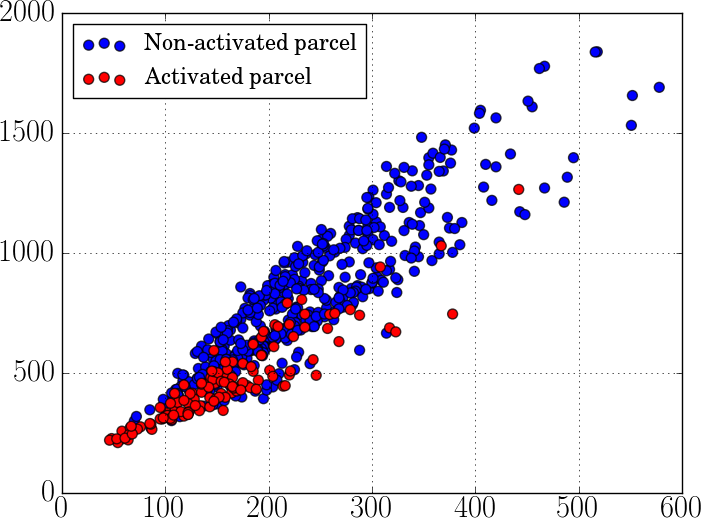
$\Delta t$ in sec.	Gain factor	1
parcel size	parcel size

Figure 14: Comparison of durations for MCMC and VEM analyses in terms of parcel size. (a): differential timing $t_{\text{MCMC}}-t_{\text{VEM}}$. (b): gain factor of VEM compared to MCMC ($t_{\text{MCMC}}/t_{\text{VEM}}$), the horizontal line indicates a gain factor of one ($t_{\text{MCMC}}=t_{\text{VEM}}$). Circles are red-colored for parcels estimated as activated, ie $\max\{(\widehat{\mu}_{1m})_{1\leq m\leq M}\}\geq 8$ and blue-colored otherwise.

VI Conclusion and future work

In this paper, we have proposed a new method for parcel-based joint detection-estimation of brain activity from fMRI data. The proposed method relies on a Variational EM algorithm as an alternative solution to intensive stochastic sampling used in previous work [16]. Compared to JDE MCMC, the proposed VEM approach does not require priors on the model parameters for inference to be carried out. However, for more robustness and to make the proposed approach completely auto-calibrated, the adopted model may be extended by injecting additional priors on some of its parameters as detailed in Appendix -D for ${\boldsymbol{\beta}}$ and $v_{\mathb{h}}$ estimation.
Illustrations on simulated and real datasets have been deeply conducted in order to evaluate the robustness of the proposed method compared to its MCMC counterpart in different experimental contexts. Simulations have shown that the proposed VEM algorithm gave more precise estimation of activation labels and NRLs especially at low input CNR, while giving similar performance for HRF estimation. Simulations have also shown that our approach was more robust to stimulus density decrease (or equivalently ISI time increase). Similar conclusions have been drawn wrt noise level and autocorrelation structure. In addition, our VEM approach gave more robust estimation of the spatial regularisation parameter and more compact activation maps that are likely to better account for functional homogeneity. These good features of the VEM approach are provided in shorter computational time than with the MCMC implementation. Simulations have also been conducted to study the computational time variation wrt the problem dimensions, which may significantly vary from one experimental context to another.
Regarding real data experiments, VEM and MCMC showed similar results with a higher specificity for the former. Although no ground truth is available in this context, these results further emphasize the interest of using VEM for a high gain in computational time. From a practical viewpoint, another advantage of the proposed algorithm lies in its simplicity. By contrast to the MCMC implementation of [15], the VEM algorithm only requires a simple stopping criterion. It is also more flexible to account for more complex situations such as those involving higher AR noise order, habituation modeling or considering three instead of two activation classes with an additional deactivation class.
To confirm the impact of the proposed approach, comparisons between the MCMC and VEM approaches should also take place at the group level. In other words, we should compare the results of random effect analyses (RFX) based on a Student t-test on mean effects. A first RFX analysis would correspond to the classical approach, in which the input data are given by the normalized effects of a standard individual SPM analysis. Subsequent analyses would take the results of the VEM and MCMC approaches for each subject as inputs to RFX analyses. In the same vein, a seminal study has been performed in [7] where group results based on JDE MCMC intra-subject analyses provide higher sensitivity than results based on GLM based intra-subject analyses. Such a group-level validation would also shed the light on the impact of the used variational approximation in VEM. In fact, no preliminary spatial smoothing is used in the JDE approach by contrast to standard fMRI analyses where this smoothing helps retrieving clearer activation clusters. In this context, the used mean field approximation especially at the E-Q step should help getting less noisy activation clusters compared to the MCMC approach. Eventually, akin to [16], the model used in our approach accounts for functional homogeneity at the parcel scale. These parcels are assumed to be an input of the proposed JDE procedure and can be a priori provided independently by any parcellation technique [29, 32]. In the present work, parcels have been extracted based on functional features extracted via a classical GLM processing supposing a canonical HRF for the entire brain. This assumption does not bias our HRF local model estimation since a large number of parcels is considered ($600$ parcels) with an average parcel size of $250$ voxels.
On real dataset, results may therefore depend on the reliability of the used parcellation technique. A sensitivity analysis has been performed in [33] on real data and for MCMC JDE version, that assesses the reliability of the used parcellation against a heavy approach where the parcellation was marginalised. Still, it would be of interest to investigate the effect of the parcellation choice in the VEM context, and more generally to extend the present framework to incorporate an automatic online parcellation strategy to better fit the fMRI data while accounting for the HRF variability across subjects, populations and experimental contexts. The current variational framework has the advantage to be easily augmented with parcel estimation as an additional layer in the hierarchical model. This will then raise the question of model selection, in particular the issue of well separating parcels at best i.e. in a sparse manner so as to capture the spatial variability in hemodynamic territories while enabling the reproducibility of parcel identification across fMRI datasets. More generally, an approach to model selection can be easily carried out within the VEM implementation as variational approximations of standard information criteria based on penalised log-evidence can be efficiently used [34].

-A E-H step:

For the E-H step, the expressions for ${\mathb{m}}_{H_{\gamma}}^{(r)}$ and ${\boldsymbol{\Sigma}}_{H_{\gamma}}^{(r)}$ are:

$${\boldsymbol{\Sigma}}_{H_{\gamma}}^{(r)} =[1/v_{\mathb{h}}^{(r-1)}{\mathb{R}}^{-1}+\sum_{j\in{\mathcal{P}}_{\gamma}}\Bigl{(}\sum_{m,m^{\prime}}v_{A_{j}^{m}A^{m^{\prime}}_{j}}^{(r-1)}{\mathb{X}}_{m}^{\mathrm{t}}{\boldsymbol{\Gamma}}_{j}^{(r-1)}{\mathb{X}}_{m^{\prime}}+\widetilde{{\mathb{S}}}_{j}^{\mathrm{t}}{\boldsymbol{\Gamma}}_{j}^{(r-1)}\widetilde{{\mathb{S}}}_{j}\Bigr{)}]^{-1}$$ (13)

$${\mathb{m}}_{H_{\gamma}}^{(r)} ={\boldsymbol{\Sigma}}_{H_{\gamma}}^{(r)}\sum_{j\in{\mathcal{P}}_{\gamma}}\widetilde{{\mathb{S}}}_{j}^{\mathrm{t}}{\boldsymbol{\Gamma}}_{j}^{(r-1)}({\mathb{y}}_{j}-{\mathb{P}}\boldsymbol{\ell}_{j}^{(r-1)}),$$ (14)

with $\widetilde{{\mathb{S}}}_{j}=\sum\limits_{m=1}^{M}m_{A_{j}^{m}}^{(r-1)}{\mathb{X}}_{m}$, $m_{A_{j}^{m}}^{(r-1)}$ and $v_{A_{j}^{m}A_{j}^{m^{\prime}}}^{(r-1)}$ denoting respectively the $m$ and $(m,m^{\prime})$ entries of the mean vector (${\mathb{m}}_{A_{j}}^{(r-1)}$) and covariance matrix (${\boldsymbol{\Sigma}}_{A_{j}}^{(r-1)}$) of the current $\widetilde{p}_{A_{j}}^{(r-1)}$.

-B E-A step:

The E-A step also leads to a Gaussian pdf for $\widetilde{p}^{(r)}_{A}$: $\widetilde{p}_{A}^{(r)}\sim\prod\limits_{j\in{\mathcal{P}}_{\gamma}}{\mathcal{N}}({\mathb{m}}_{A_{j}}^{(r)},{\boldsymbol{\Sigma}}_{A_{j}}^{(r)})$. The parameters are updated as follows:

$${\boldsymbol{\Sigma}}_{A_{j}}^{(r)}=\Bigl{(}\sum\limits_{i=1}^{I}{\boldsymbol{\Delta}}_{ij}+\widetilde{{\mathb{H}}}_{j}\Bigr{)}^{-1} {\mathb{m}}_{A_{j}}^{(r)}={\boldsymbol{\Sigma}}_{A_{j}}^{(r)}\;\Bigl{(}\sum\limits_{i=1}^{I}{\boldsymbol{\Delta}}_{ij}{\boldsymbol{\mu}}^{(r-1)}_{i}+\widetilde{{\mathb{G}}}^{\mathrm{t}}{\boldsymbol{\Gamma}}_{j}^{(r-1)}({\mathb{y}}_{j}-{\mathb{P}}\boldsymbol{\ell}_{j}^{(r-1)})\Bigr{)}$$ , (15)

where a number of intermediate quantities need to be specified. First, ${\boldsymbol{\mu}}^{(r-1)}_{i}=\left[\mu_{i1}^{(r-1)},\ldots,\mu_{iM}^{(r-1)}\right]^{\mathrm{t}}$ and $\widetilde{{\mathb{G}}}={\mathrm{E}}_{\widetilde{p}_{H_{\gamma}}^{(r)}}\bigl{[}{\mathb{G}}\bigr{]}$ where ${\mathb{G}}$ is the matrix ${\mathb{G}}=\left[{\mathb{g}}_{1}\,|\,\ldots\,|\,{\mathb{g}}_{M}\right]$ made of columns ${\mathb{g}}_{m}={\mathb{X}}_{m}{\mathb{h}}_{\gamma}$. The $m$-th column of $\widetilde{{\mathb{G}}}$ is then also denoted by $\widetilde{{\mathb{g}}}_{m}={\mathb{X}}_{m}{\mathb{m}}_{H_{\gamma}}^{(r)}\in\mathbb{R}^{N}$. Then, ${\boldsymbol{\Delta}}_{ij}={\mathrm{diag}}_{M}\left[\widetilde{p}_{Q_{j}^{m}}^{(r-1)}(i)/v_{im}^{(r-1)}\right]$ and $\widetilde{{\mathb{H}}}_{j}={\mathrm{E}}_{\widetilde{p}_{H_{\gamma}}^{(r)}}\bigl{[}{\mathb{G}}^{\mathrm{t}}{\boldsymbol{\Gamma}}_{j}^{(r-1)}{\mathb{G}}\bigr{]}$ is an $M\times M$ matrix whose element $(m,m^{\prime})$ is given by:

$${\mathrm{E}}_{\widetilde{p}_{H_{\gamma}}^{(r)}}\bigl{[}{\mathb{g}}_{m}^{\mathrm{t}}{\boldsymbol{\Gamma}}_{j}^{(r-1)}{\mathb{g}}_{m^{\prime}}\bigr{]} ={\mathrm{E}}_{\widetilde{p}_{H_{\gamma}}^{(r)}}\bigl{[}{\mathb{g}}_{m}\bigr{]}^{\mathrm{t}}{\boldsymbol{\Gamma}}_{j}^{(r-1)}{\mathrm{E}}_{\widetilde{p}_{H_{\gamma}}^{(r)}}\bigl{[}{\mathb{g}}_{m^{\prime}}\bigr{]}+\mathrm{trace}\bigl{(}{\boldsymbol{\Gamma}}_{j}^{(r-1)}cov_{\widetilde{p}_{H_{\gamma}}^{(r)}}({\mathb{g}}_{m},{\mathb{g}}_{m^{\prime}})\bigr{)}$$

$$=\widetilde{{\mathb{g}}}_{m}^{\mathrm{t}}{\boldsymbol{\Gamma}}_{j}^{(r-1)}\widetilde{{\mathb{g}}}_{m^{\prime}}+\mathrm{trace}\bigl{(}{\boldsymbol{\Gamma}}_{j}^{(r-1)}{\mathb{X}}_{m}{\boldsymbol{\Sigma}}_{H_{\gamma}}^{(r)}{\mathb{X}}^{\mathrm{t}}_{m^{\prime}}\bigr{)}.$$

-C E-Q step:

From $p({\mathb{A}}|{\mathb{Q}})$ and $p({\mathb{Q}})$ in Section II, it follows that the $({\mathb{a}}^{m},{\mathb{q}}^{m})$ couples correspond to independent hidden Potts models with Gaussian class distributions. It follows an approximation that factorizes over conditions: $\widetilde{p}^{(r)}_{Q}({\mathb{Q}})\!=\!\!\prod\limits_{m=1}^{M}\widetilde{p}^{(r)}_{Q^{m}}({\mathb{q}}^{m})$ where $\widetilde{p}^{(r)}_{Q^{m}}({\mathb{q}}^{m})\!=\!f({\mathb{q}}^{m}|{\mathb{a}}^{m}\!=\!{\mathb{m}}_{A^{m}}^{(r)};{\boldsymbol{\mu}}_{m}^{(r-1)},{\mathb{v}}_{m}^{(r-1)},\beta_{m}^{(r-1)})$ is the posterior of ${\mathb{q}}^{m}$ in a modified hidden Potts model $f$, in which the observations $a_{j}^{m}$’s are replaced by their mean values ${\mathb{m}}^{(r)}_{A_{j}^{m}}$ and an external field $\{{\boldsymbol{\alpha}}_{j}^{m(r)}=v_{A_{j}^{m}A_{j}^{m}}^{(r)}\left[1/v^{(r-1)}_{{1m}},\ldots,1/v^{(r-1)}_{{Im}}\right]^{\mathrm{t}},\quad\linebreak j\in{\mathcal{P}}_{\gamma}\}$ is added to the prior Potts model $p({\mathb{q}}^{m};\beta^{(r-1)}_{m})$. It follows that the defined Potts reads:

$$f({\mathb{q}}^{m};{\mathb{v}}^{(r-1)}_{m},\beta^{(r-1)}_{m})\propto\exp\{\sum_{j\in{\mathcal{P}}_{\gamma}}\Big{(}{\boldsymbol{\alpha}}_{j}^{m(r)}(q_{j}^{m})+\frac{1}{2}\beta^{(r-1)}_{m}\sum_{k\sim j}{\delta(q_{j}^{m},q_{k}^{m})}\Big{)}\}.$$ (16)

Since the expression in Eq. (16) is intractable, and using the mean-field approximation [26], $\widetilde{p}_{Q^{m}}^{(r)}({\mathb{q}}^{m})$ is approximated by a factorized density $\widetilde{p}_{Q^{m}}^{(r)}({\mathb{q}}^{m})=\prod\limits_{j\in{\mathcal{P}}_{\gamma}}\widetilde{p}_{Q_{j}^{m}}^{(r)}(q_{j}^{m})$ such that if $q_{j}^{m}=i$,

$$\widetilde{p}_{Q_{j}^{m}}^{(r)}(i)\propto{\mathcal{N}}({\mathb{m}}_{A_{j}^{m}}^{(r)};\mu_{im}^{(r-1)},v_{im}^{(r-1)})f(q_{j}^{m}=i\,|\,\tilde{q}_{\sim j}^{m};\beta_{m}^{(r-1)},{\mathb{v}}_{m}^{(r-1)}),$$ (17)

where $\tilde{{\mathb{q}}}^{m}$ is a particular configuration of ${\mathb{q}}^{m}$ updated at each iteration according to a specific scheme and $f(q_{j}^{m}\,|\,\tilde{q}_{\sim j}^{m};\beta_{m}^{(r-1)},{\mathb{v}}_{m}^{(r-1)})\propto\exp\{{\boldsymbol{\alpha}}_{j}^{m(r)}(q_{j}^{m})+\beta_{m}^{(r-1)}\sum\limits_{k\sim j}{\delta(\tilde{q}_{k}^{m},q_{j}^{m})}\}$.

-D M step:

-D1 M-$({\boldsymbol{\mu}},{\mathb{v}})$ step

By maximizing with respect to $({\boldsymbol{\mu}},{\mathb{v}})$, Eq. (• ‣ III) reads:

$$({\boldsymbol{\mu}}^{(r)},{\mathb{v}}^{(r)}) =\mathop{\mathrm{arg\,max}}_{({\boldsymbol{\mu}},{\mathb{v}})}\;{\mathrm{E}}_{\widetilde{p}_{A}^{(r)}\widetilde{p}_{Q}^{(r)}}\bigl{[}\log p({\mathb{A}}\,|\,{\mathb{Q}};{\boldsymbol{\mu}},{\mathb{v}})\bigr{]}$$ (18)

By denoting $\bar{p}^{(r)}_{im}=\sum\limits_{j\in{\mathcal{P}}_{\gamma}}\widetilde{p}^{(r)}_{Q_{j}^{m}}(i)$, and after deriving wrt $\mu_{im}$ and $v_{im}$ for every $i\in\{1\ldots I\}$ and $m\in\{1\ldots M\}$, we get $\mu^{(r)}_{im}={\sum\limits_{j\in{\mathcal{P}}_{\gamma}}p^{(r)}_{Q_{j}^{m}}(i)\;m^{(r)}_{A_{j}^{m}}/\bar{p}^{(r)}_{im}}$ and $v^{(r)}_{im}={\sum\limits_{j\in{\mathcal{P}}_{\gamma}}\widetilde{p}^{(r)}_{Q_{j}^{m}}(i)\bigl{(}(m^{(r)}_{A_{j}^{m}}-\mu^{(r)}_{im})^{2}+v^{(r)}_{A_{m}^{j}A_{m}^{j}}\bigr{)}/\bar{p}^{(r)}_{im}}$.

-D2 M-$v_{\mathb{h}}$ step

By maximizing with respect to $v_{\mathb{h}}$, Eq. (• ‣ III) reads:

$$v_{\mathb{h}}^{(r)} =\mathop{\mathrm{arg\,max}}_{v_{\mathb{h}}}\;{\mathrm{E}}_{\widetilde{p}_{H_{\gamma}}^{(r)}}\bigl{[}\log p({\mathb{h}}_{\gamma};{\mathb{v}}_{h})\bigr{]}.$$ (19)

It follows the closed-form expression given by

$$v_{\mathb{h}}^{(r)} =\frac{{\mathrm{E}}_{\widetilde{p}_{H_{\gamma}}^{(r)}}\bigl{[}{\mathb{h}}_{\gamma}^{\mathrm{t}}{\mathb{R}}^{-1}{\mathb{h}}_{\gamma}\bigr{]}}{(D-1)}=\frac{({\mathb{m}}_{H_{\gamma}}^{(r)t}{\mathb{R}}^{-1}{\mathb{m}}_{H_{\gamma}}^{(r)}\!+\mathrm{trace}({\boldsymbol{\Sigma}}_{H_{\gamma}}^{(r)}{\mathb{R}}^{-1}))}{(D-1)}=\frac{\mathrm{trace}(({\boldsymbol{\Sigma}}_{H_{\gamma}}^{(r)}+{\mathb{m}}_{H_{\gamma}}^{(r)}{\mathb{m}}_{H_{\gamma}}^{(r)t}){\mathb{R}}^{-1})}{(D-1)}.$$ (20)

For a more accurate estimation of $v_{\mathb{h}}$, one may take advantage of the flexibility of the VEM inference and inject some prior knowledge about this parameter in the model. Since this parameter is positive, a suitable prior can be an exponential distribution with mean $\lambda_{v_{\mathb{h}}}^{-1}$:

$$p(v_{\mathb{h}};\lambda_{v_{\mathb{h}}})=\lambda_{v_{\mathb{h}}}\exp\{-\lambda_{v_{\mathb{h}}}v_{\mathb{h}}\}.$$ (21)

Taking this prior into account, the new expression of the current estimate $v_{\mathb{h}}^{(r)}$ is:

• $v_{\mathb{h}}^{(r)}=\frac{(D-1)+\sqrt{8\lambda_{v_{\mathb{h}}}C+(D-1)^{2}}}{4\lambda_{v_{\mathb{h}}}}$ with $C=\mathrm{trace}(({\boldsymbol{\Sigma}}_{H_{\gamma}}^{(r)}+{\mathb{m}}_{H_{\gamma}}^{(r)}{{\mathb{m}}^{(r)}_{H_{\gamma}}}^{t}){\mathb{R}}^{-1})$

-D3 M-${\boldsymbol{\beta}}$ step

By maximizing with respect to ${\boldsymbol{\beta}}$, Eq. (• ‣ III) reads:

$${\boldsymbol{\beta}}^{(r)} =\mathop{\mathrm{arg\,max}}_{{\boldsymbol{\beta}}}\;{\mathrm{E}}_{\widetilde{p}_{Q}^{(r)}}\bigl{[}\log p({\mathb{Q}};{\boldsymbol{\beta}})\bigr{]}.$$ (22)

Updating ${\boldsymbol{\beta}}$ consists of making further use of a mean field-like approximation [26], which leads to a function that can be optimized using a gradient algorithm. To avoid over-estimation of this key parameter for the spatial regularisation, one can introduce for each $\beta_{m}$, some prior knowledge $p(\beta_{m};\lambda_{\beta_{m}})$ that penalises high values. As in Eq. (21), an exponential prior with mean $\lambda_{\beta_{m}}^{-1}$ can be used. The expression to optimize is then given by:

$$\beta^{(r)}_{m} =\arg\max\limits_{\beta_{m}}E_{\widetilde{p}_{Q^{m}}^{(r)}}[\log p({\mathb{q}}^{m};\beta_{m})p(\beta_{m};\lambda_{\beta_{m}})]$$

$$=\arg\max\limits_{\beta_{m}}\{-\log Z(\beta_{m})+\beta_{m}(\sum\limits_{j\thicksim k}{\mathrm{E}}_{\widetilde{p}^{(r)}_{Q^{m}}}\bigl{[}{\delta(q_{j}^{m},q_{k}^{m})}\bigr{]}-\lambda_{\beta_{m}})\}.$$ (23)

After calculating the derivative wrt $\beta_{m}$, we retrieve the standard equation detailed in [26] in which $\sum\limits_{j\thicksim k}{\mathrm{E}}_{\widetilde{p}^{(r)}_{Q^{m}}}\bigl{[}{\delta(q_{j}^{m},q_{k}^{m})}\bigr{]}$ is replaced by $\sum\limits_{j\thicksim k}{\mathrm{E}}_{\widetilde{p}^{(r)}_{Q^{m}}}\bigl{[}{\delta(q_{j}^{m},q_{k}^{m})}\bigr{]}-\lambda_{\beta_{m}}$. It can be easily seen that, as expected, subtracting the constant $\lambda_{\beta_{m}}$ helps penalizing high $\beta_{m}$ values.

-D4 M-$({\mathb{L}},{\boldsymbol{\Gamma}})$ step

This maximization problem factorizes over voxels so that for each $j\in{\mathcal{P}}_{\gamma}$, we need to compute:

$$(\boldsymbol{\ell}^{(r)}_{j},{\boldsymbol{\Gamma}}^{(r)}_{j}) =\mathop{\mathrm{arg\,max}}\limits_{(\boldsymbol{\ell}_{j},{\boldsymbol{\Gamma}}_{j})}\;{\mathrm{E}}_{\widetilde{p}_{H_{\gamma}}^{(r)}\widetilde{p}_{A_{j}}^{(r)}}\bigl{[}\log p({\mathb{y}}_{j}\,|\,{\mathb{a}}_{j},{\mathb{h}}_{\gamma};\boldsymbol{\ell}_{j},{\boldsymbol{\Gamma}}_{j})\bigr{]}\;,$$ (24)

where ${\mathb{a}}_{j}=\{a_{j}^{m},m=1\ldots M\}$. Finding the maximizer wrt $\boldsymbol{\ell}_{j}$ leads to ($\widetilde{{\mathb{G}}}$ is defined in the E-A step):

$$\boldsymbol{\ell}^{(r)}_{j} =\mathop{\mathrm{arg\,max}}\limits_{\boldsymbol{\ell}_{j}}\{2(\widetilde{{\mathb{G}}}{\mathb{m}}_{A_{j}}^{(r)}-{\mathb{y}}_{j})^{\mathrm{t}}{\boldsymbol{\Gamma}}^{(r)}_{j}{\mathb{P}}\boldsymbol{\ell}_{j}+\boldsymbol{\ell}_{j}^{\mathrm{t}}{\mathb{P}}^{\mathrm{t}}{\boldsymbol{\Gamma}}^{(r)}_{j}{\mathb{P}}\boldsymbol{\ell}_{j}\}.$$ (25)

After calculating the derivative wrt $\boldsymbol{\ell}_{j}$, we get $\boldsymbol{\ell}^{(r)}_{j}=({\mathb{P}}^{\mathrm{t}}{\boldsymbol{\Gamma}}^{(r)}_{j}{\mathb{P}})^{-1}{\mathb{P}}^{\mathrm{t}}{\boldsymbol{\Gamma}}^{(r)}_{j}({\mathb{y}}_{j}-\widetilde{{\mathb{G}}}{\mathb{m}}_{A_{j}}^{(r)})$. In the AR(1) case, with ${\boldsymbol{\Gamma}}_{j}=\sigma_{j}^{-2}{\boldsymbol{\Lambda}}_{j}$, we can then derive the following relationship:

$$\boldsymbol{\ell}^{(r)}_{j} =({\mathb{P}}^{\mathrm{t}}{\boldsymbol{\Lambda}}^{(r)}_{j}{\mathb{P}})^{-1}{\mathb{P}}^{\mathrm{t}}{\boldsymbol{\Lambda}}^{(r)}_{j}\biggl{(}y_{j}-\widetilde{{\mathb{S}}}_{j}m_{H_{\gamma}}^{(r)}\biggr{)}F_{1}(\rho^{(r)}_{j}),$$ (26)

where $F_{1}$ is a function linking the estimates $\boldsymbol{\ell}^{(r)}_{j}$ and $\rho^{(r)}_{j}$. The above formula is similar to that in [16, p.965, B.2], when replacing ${\mathb{h}}_{\gamma}$ by $m_{H_{\gamma}}^{(r)}$ and ${\mathb{a}}$ by $m_{A}^{(r)}$.

Denoting ${\mathb{y}}^{(r)}_{j}={\mathb{y}}_{j}-{\mathb{P}}\boldsymbol{\ell}^{(r)}_{j}$ and considering the maximization wrt $\sigma^{2}_{j}$, similar calculations lead to:

$$\sigma^{2(r)}_{j}=\frac{1}{N}\left({\mathrm{E}}_{\widetilde{p}_{A_{j}}^{(r)}}\bigl{[}{\mathb{a}}_{j}^{t}\widetilde{{\boldsymbol{\Lambda}}}_{j}^{(r)}{\mathb{a}}_{j}\bigr{]}-2{\mathb{m}}_{A_{j}}^{(r)t}\widetilde{{\mathb{G}}}{\boldsymbol{\Lambda}}^{(r)}_{j}{\mathb{y}}^{(r)}_{j}+{\mathb{y}}^{(r)t}_{j}{\boldsymbol{\Lambda}}^{(r)}_{j}{\mathb{y}}^{(r)}_{j}\right)=F_{2}(\rho^{(r)}_{j},\boldsymbol{\ell}^{(r)}_{j}),$$ (27)

where $F_{2}$ is a function linking the estimates $\sigma^{2(r)}_{j}$ with $\boldsymbol{\ell}^{(r)}_{j}$ and $\rho^{(r)}_{j}$. Matrix $\widetilde{{\boldsymbol{\Lambda}}}^{(r)}_{j}={\mathrm{E}}_{\widetilde{p}_{H_{\gamma}}^{(r)}}\bigl{[}{\mathb{G}}^{\mathrm{t}}{\boldsymbol{\Lambda}}^{(r)}_{j}{\mathb{G}}\bigr{]}$ is a $M\times M$ matrix similar to the matrix $\widetilde{{\mathb{H}}}_{j}$ introduced in the E-A step. Its $(m,m^{\prime})$ entry is given by $\widetilde{{\mathb{g}}}_{m}^{\mathrm{t}}{\boldsymbol{\Lambda}}_{j}^{(r)}\widetilde{{\mathb{g}}}_{m^{\prime}}+\mathrm{trace}\bigl{(}{\boldsymbol{\Lambda}}_{j}^{(r)}{\mathb{X}}_{m}{\boldsymbol{\Sigma}}_{H_{\gamma}}^{(r)}{\mathb{X}}^{\mathrm{t}}_{m^{\prime}}\bigr{)}.$
Eventually, the maximization wrt $\rho_{j}$ leads to $\rho^{(r)}_{j}=\mathop{\mathrm{arg\,max}}\limits_{\rho_{j}}\{\bigl{(}\mathrm{trace}({\mathb{U}}_{1}\widetilde{\Lambda_{j}})+\mathrm{trace}({\mathb{U}}_{2}\Lambda_{j})\bigr{)}/\sigma_{j}^{2(r)}+\log|\Lambda_{j}|\},$ with $|\Lambda_{j}|=1-\rho_{j}^{2}$ and where $\widetilde{\Lambda_{j}}$ has the same expression as $\widetilde{{\boldsymbol{\Lambda}}}^{(r)}_{j}$ without the $(r)$ superscript. Matrices ${\mathb{U}}_{1}$ and ${\mathb{U}}_{2}$ are respectively $M\times M$ and $N\times N$ matrices defined as ${\mathb{U}}_{1}={\boldsymbol{\Sigma}}^{(r)}_{A_{j}}+{\mathb{m}}_{A_{j}}^{(r)}{{\mathb{m}}_{A_{j}}^{(r)}}^{\mathrm{t}}$ and ${\mathb{U}}_{2}={\mathb{y}}_{j}^{(r)}({\mathb{y}}_{j}^{(r)}-2\widetilde{{\mathb{G}}}{\mathb{m}}_{A_{j}}^{(r)})^{\mathrm{t}}$. The derivative, denoted by $\Lambda_{j}$ of $\Lambda_{j}$ wrt $\rho_{j}$ writes $\Lambda_{j}^{\prime}=2\rho_{j}{\mathb{B}}+{\mathb{C}}$, where the entries of ${\mathb{B}}$ and ${\mathb{C}}$ are zero except $({\mathb{B}})_{n,n}$ which is 1 for $n=2:(N-1)$ and for $({\mathb{C}})_{n,n+1}$ and $({\mathb{C}})_{n+1,n}$ which are -1 for $n=1:(N-1)$. The derivative, denoted by $\widetilde{\Lambda}_{j}^{\prime}$, of $\widetilde{\Lambda}_{j}$ wrt $\rho_{j}$ can be written as: $\widetilde{\Lambda}_{j}^{\prime}=2\rho_{j}\widetilde{{\mathb{B}}}+\widetilde{{\mathb{C}}}$ where $\widetilde{{\mathb{B}}}$ and $\widetilde{{\mathb{C}}}$ are $M\times M$ matrices whose entries $(m,m^{\prime})$ are respectively $(\widetilde{{\mathb{B}}})_{m,m^{\prime}}=\mathrm{trace}\bigl{(}({\mathb{X}}_{m}{\boldsymbol{\Sigma}}_{{\mathb{H}}_{\gamma}}^{(r)}{\mathb{X}}_{m^{\prime}}^{\mathrm{t}}+\widetilde{{\mathb{g}}}_{m^{\prime}}\widetilde{{\mathb{g}}}_{m}^{\mathrm{t}}){\mathb{B}}\bigr{)}$ and $(\widetilde{{\mathb{C}}})_{m,m^{\prime}}=\mathrm{trace}\bigl{(}({\mathb{X}}_{m}{\boldsymbol{\Sigma}}_{{\mathb{H}}_{\gamma}}^{(r)}{\mathb{X}}_{m^{\prime}}^{\mathrm{t}}+\widetilde{{\mathb{g}}}_{m^{\prime}}\widetilde{{\mathb{g}}}_{m}^{\mathrm{t}}){\mathb{C}}\bigr{)}$. Eventually, the derivative wrt $\rho_{j}$ leads to:

$$\rho_{j}^{(r)}=\frac{1-\rho_{j}^{(r)}}{\sigma_{j}^{2(r)}}\{2\rho_{j}^{(r)}\bigl{(}\mathrm{trace}({\mathb{U}}_{1}\widetilde{{\mathb{B}}})+\mathrm{trace}({\mathb{U}}_{2}{\mathb{B}})\bigr{)}+\mathrm{trace}({\mathb{U}}_{1}\widetilde{{\mathb{C}}})+\mathrm{trace}({\mathb{U}}_{2}{\mathb{C}})\}=F_{3}(\rho_{j}^{(r)},\sigma_{j}^{2(r)}).$$

Then $\rho_{j}^{(r)}$ can be estimated as a solution of the fixed point equation $\rho_{j}^{(r)}=F_{3}(\rho_{j}^{(r)},F_{2}(\rho_{j}^{(r)},F_{1}(\rho_{j}^{(r)}))).$ Note that in the Gaussian noise case, the updating of the noise parameters reduces to the estimation of $\sigma_{j}^{2(r)}$ which simplifies into $\sigma_{j}^{2(r)}=\frac{1}{N}\left({\mathrm{E}}_{\widetilde{p}_{A_{j}}^{(r)}}\bigl{[}{\mathb{a}}_{j}^{t}{\mathrm{E}}_{\widetilde{p}_{H_{\gamma}}^{(r)}}\bigl{[}{\mathb{G}}^{\mathrm{t}}{\mathb{G}}\bigr{]}{\mathb{a}}_{j}\bigr{]}-2{\mathb{m}}_{A_{j}}^{(r)t}\widetilde{{\mathb{G}}}{\mathb{y}}^{(r)}_{j}+{\mathb{y}}^{(r)t}_{j}{\mathb{y}}^{(r)}_{j}\right)$.

References

- [1] S. Ogawa, T. M. Lee, A. R. Kay, and D. W. Tank, “Brain magnetic resonance imaging with contrast dependent on blood oxygenation,” Nat. Acad. Sci., vol. 87, pp. 9868–72, 1990.
- [2] R. Buxton and L. Frank, “A model for the coupling between cerebral blood flow and oxygen metabolism during neural stimulation,” J. Cereb. Blood Flow Metab., vol. 17, no. 1, pp. 64–72, 1997.
- [3] J. J. Riera, J. Bosch, O. Yamashita, R. Kawashima, N. Sadato, T. Okada, and T. Ozaki, “fMRI activation maps based on the NN-ARx model,” Neuroimage, vol. 23, pp. 680–697, 2004.
- [4] G. M. Boynton, S. A. Engel, G. H. Glover, and D. J. Heeger, “Linear systems analysis of functional magnetic resonance imaging in human V1,” J. Neurosci., vol. 16, pp. 4207–4221, 1996.
- [5] K. J. Friston, P. Jezzard, and R. Turner, “Analysis of functional MRI time-series,” Hum. Brain Mapp., vol. 1, pp. 153–171, 1994.
- [6] D. A. Handwerker, J. M. Ollinger, and D. Mark, “Variation of BOLD hemodynamic responses across subjects and brain regions and their effects on statistical analyses,” Neuroimage, vol. 21, pp. 1639–1651, 2004.
- [7] S. Badillo, T. Vincent, and P. Ciuciu, “Impact of the joint detection-estimation approach on random effects group studies in fMRI,” in Int. Symp. on Biomed. Imaging, Chicago, IL, USA, avr. 2011, pp. 376–380.
- [8] R. Henson, M. Rugg, and K. Friston, “The choice of basis function in event-related fMRI,” 2001, vol. 13, p. 149.
- [9] C. Goutte, F. Nielsen, and L. K. Hansen, “Modeling the haemodynamic response in fMRI using smooth FIR filters,” IEEE Transactions on Medical Imaging, vol. 19, no. 12, pp. 1188–1201, Dec. 2000.
- [10] P. Ciuciu, J. Idier, G. Flandin, G. Marrelec, and J.-B. Poline, “On the spatial variability of the BOLD HRF and some regularization strategies,” in Hum. Brain Mapp., New York, Jun. 19-22 2003.
- [11] J. Kershaw, B. A. Ardekani, and I. Kanno, “Application of Bayesian inference to fMRI data analysis,” IEEE Trans. Med. Imag., vol. 18, no. 12, pp. 1138–1152, Dec. 1999.
- [12] S. Makni, P. Ciuciu, J. Idier, and J.-B. Poline, “Joint detection-estimation of brain activity in functional MRI: a multichannel deconvolution solution,” IEEE Trans. Signal Process., vol. 53, no. 9, pp. 3488–3502, Sep. 2005.
- [13] F. de Pasquale, C. Del Gratta, and G. L. Romani, “Empirical markov chain monte carlo bayesian analysis of fMRI data,” Neuroimage, vol. 42, no. 1, pp. 99–111, Aug. 2008.
- [14] S. Makni, C. Beckmann, S. Smith, and M. Woolrich, “Bayesian deconvolution of fMRI data using bilinear dynamical systems,” Neuroimage, vol. 42, no. 4, pp. 1381–1396, 2008.
- [15] T. Vincent, L. Risser, and P. Ciuciu, “Spatially adaptive mixture modeling for analysis of within-subject fMRI time series,” IEEE Trans. Med. Imag., vol. 29, pp. 1059–1074, 2010.
- [16] S. Makni, J. Idier, T. Vincent, B. Thirion, G. Dehaene-Lambertz, and P. Ciuciu, “A fully Bayesian approach to the parcel-based detection-estimation of brain activity in fMRI,” Neuroimage, vol. 41, no. 3, pp. 941–969, 2008.
- [17] W. D. Penny, S. Kiebel, and K. J. Friston, “Variational Bayesian inference for fMRI time series,” Neuroimage, vol. 19, no. 3, pp. 727–741, 2003.
- [18] K. J. Friston, J. Mattout, N. Trullijo-Barreto, J. Ashburner, and W. Penny, “Variational free energy and the Laplace approximation,” Neuroimage, vol. 33, pp. 220–234, 2007.
- [19] M. Woolrich and T. Behrens, “Variational Bayes inference of spatial mixture models for segmentation,” IEEE Trans. Med. Imag., vol. 25, no. 10, pp. 1380–1391, oct. 2006.
- [20] M. Woolrich, B. Ripley, M. Brady, and S. Smith, “Temporal autocorrelation in univariate linear modelling of fMRI data,” Neuroimage, vol. 14, no. 6, pp. 1370–1386, Dec. 2001.
- [21] S. Makni, P. Ciuciu, J. Idier, and J.-B. Poline, “Joint detection-estimation of brain activity in fmri using an autoregressive noise model,” in IEEE Int. Symp. on Biomed. Imag. (ISBI), Arlington, VA, 6-9 April 2006, pp. 1048 – 1051.
- [22] M. Woolrich, M. Jenkinson, J. Brady, and S. Smith, “Fully Bayesian spatio-temporal modelling of fMRI data,” IEEE Trans. Med. Imag., vol. 23, no. 2, pp. 213–231, Feb. 2004.
- [23] W. D. Penny, G. Flandin, and N. Trujillo-Bareto, “Bayesian Comparison of Spatially Regularised General Linear Models,” Hum. Brain Mapp., vol. 28, no. 4, pp. 275–293, 2007.
- [24] R. M. Neal and G. E. Hinton, “A view of the EM algorithm that justifies incremental, sparse and other variants,” in Lear. in Graph. Mod., Jordan, Ed., pp. 355–368. 1998.
- [25] M. Beal and Z. Ghahramani, The variational Bayesian EM Algorithm for incomplete data: with application to scoring graphical model structures, Bay. Stat. Oxford University Press, 2003.
- [26] G. Celeux, F. Forbes, and N. Peyrard, “EM procedures using mean field-like approximations for Markov model-based image segmentation,” Patt. Rec., vol. 36, pp. 131–144, 2003.
- [27] R. Casanova, S. Ryali, J. Serences, L. Yang, R. Kraft, P. J. Laurienti, and J. A. Maldjian, “The impact of temporal regularization on estimates of the BOLD hemodynamic response function: a comparative analysis,” Neuroimage, vol. 40, no. 4, pp. 1606–1618, May 2008.
- [28] P. Pinel, B. Thirion, S. Mériaux, A. Jobert, J. Serres, D. Le Bihan, J.-B. Poline, and S. Dehaene, “Fast reproducible identification and large-scale databasing of individual functional cognitive networks,” BMC Neurosci., vol. 8, no. 1, pp. 91, 2007.
- [29] B. Thirion, G. Flandin, P. Pinel, A. Roche, P. Ciuciu, and J.-B. Poline, “Dealing with the shortcomings of spatial normaliza-tion: Multi-subject parcellation of fMRI datasets,” Hum. Brain Mapp., vol. 27, no. 8, pp. 678–693, 2006.
- [30] O. Gruber, P. Indefrey, H. Steinmetz, and A. Kleinschmidt, “Dissociating Neural Correlates of Cognitive Components in Mental Calculation,” Cereb. Cortex, vol. 11, no. 4, pp. 350–359, 2001.
- [31] A. Gelman and D. B. Rubin, “Inference from iterative simulation using multiple sequences,” Stat. Science, vol. 7, no. 4, pp. 457–472, Nov. 1992.
- [32] A. Tucholka, B. Thirion, M. Perrot, P. Pinel, J.-F. Mangin, and J.-B. Poline, “Probabilistic anatomo-functional parcellation of the cortex: how many regions?,” in 11thProc. MICCAI, LNCS Springer Verlag, New-York, USA, 2008.
- [33] T. Vincent, P. Ciuciu, and B. Thirion, “Sensitivity analysis of parcellation in the joint detection-estimation of brain activity in fMRI,” in 5th IEEE Int. Symp. on Biomed. Imag. (ISBI), Paris, France, mai 2008, pp. 568–571.
- [34] F. Forbes and N. Peyrard, “Hidden Markov Random Field model selection criteria based on mean field-like approximations,” IEEE Trans. Pattern Anal. Mach. Intell., vol. 25, no. 9, pp. 1089–1101, sep. 2003.