Radial Migration in Galactic Thick Discs

Abstract

We present a study of the extent to which the Sellwood & Binney radial migration of stars is affected by their vertical motion about the midplane. We use both controlled simulations in which only a single spiral mode is excited, as well as slightly more realistic cases with multiple spiral patterns and a bar. We find that rms angular momentum changes are reduced by vertical motion, but rather gradually, and the maximum changes are almost as large for thick disc stars as for those in a thin disc. We find that particles in simulations in which a bar forms suffer slightly larger angular momentum changes than in comparable cases with no bar, but the cumulative effect of multiple spiral events still dominates. We have determined that vertical action, and not vertical energy, is conserved on average during radial migration.

1 Introduction

It has recently become clear that galaxy discs evolve significantly over time due to both internal and external influences (see van der Kruit & Freeman, 2011; Sellwood, 2010, for reviews). Scattering by giant molecular clouds (e.g. Spitzer & Schwarzschild, 1953) is now thought to play a minor role (Hänninen & Flynn, 2002), while spirals (Sellwood & Carlberg, 1984; Binney & Lacey, 1988; Sellwood & Binney, 2002) and interactions (Helmi et al., 2006; Kazantzidis et al., 2008) are believed to cause more substantial changes.

The Milky Way is believed to have both a thin and a thick disc (Gilmore & Reid, 1983; Munn et al., 2004; Jurić et al., 2008; Ivezić et al., 2008), as do perhaps many disc galaxies (Yoachim & Dalcanton, 2006). Relative to the thin disc, the thick disc has a higher velocity dispersion, lags in its net rotational velocity (Chiba & Beers, 2000), contains older stars with lower metallicities (Majewski, 1993) and enhanced [$\alpha$/Fe] ratios (Bensby et al., 2005; Reddy, Lambert & Allende Prieto, 2006; Fuhrmann, 2008). A number of different criteria have been used to divide stars into the two disc populations, and some of these trends may depend somewhat on whether a spatial, kinematic, or chemical abundance criterion is applied (Fuhrmann, 2008; Schönrich & Binney, 2009b; Lee et al., 2011). Recently, Bovy et al. (2011) suggest that there is no sharp distinction into two populations, but rather a continuous variation in these properties.

Several models have been proposed for the formation of the thick disc: accretion of disrupted satellite galaxies (Abadi et al., 2003), thickening of an early thin disc by a minor merger (Quinn, Hernquist & Fullagar, 1993; Villalobos & Helmi, 2008), star formation triggered during galaxy assembly (Brook et al., 2005; Bournaud, Elmegreen & Martig, 2009), and radial migration (Schönrich & Binney, 2009a; Loebman et al., 2011). While it is likely that no single mechanism plays a unique role in its formation, our focus in this paper is on radial migration.

As first shown by Sellwood & Binney (2002), spiral activity in a disc causes stars to diffuse radially over time. Stars near corotation of a spiral pattern experience large angular momentum changes of either sign that move them to new radii without adding random motion. As spirals are recurring transient disturbances that have corotation radii scattered over a wide swath of the disc, the net effect is that stars execute a random walk in radius with a step size ranging up to $\sim 2\;$kpc, which results in strong radial mixing. Note that this mechanism is distinct from the “blurring” caused by epicycle oscillations of stars about their home radii, $R_{h}$, where $L_{z}^{2}=R_{h}^{3}|\partial\Phi/\partial R|_{R_{h}}$ in the midplane and $\Phi$ is the gravitational potential. Radial mixing is dubbed “churning” and causes the home radii themselves to change.

Note that radial mixing caused by recurrent transient spirals has two related properties that distinguish it from other processes that have sometimes also been said to cause radial migration. The two distinctive properties are the absence of disc heating, already noted, and the fact that stars mostly change places, causing little change to the distribution of angular momentum within the disc and leaving the surface density profile unchanged. These are both features of scattering at corotation; spirals also cause smaller angular momentum changes at Lindblad resonances which do heat and spread the disc.

Bar formation causes greater angular momentum changes than those of an individual spiral pattern (Friedli, Benz & Kennicutt, 1994; Raboud et al., 1998; Grenon, 1999; Debattista et al., 2006; Minchev et al., 2011; Bird, Kazantzidis & Weinberg, 2011; Brunetti et al., 2011). However, because the bar persists after its formation, the associated angular momentum changes have a different character from those caused by a spiral that grows and decays quickly. Bar formation changes the radial distribution of angular momentum, and therefore also the surface density profile of the disc, as well as adding a substantial amount of radial motion (Hohl, 1971). Although the bar may subsequently settle, grow, and/or slow down over time, the main changes associated with its formation probably occur only once in a galaxy’s lifetime (for a dissenting view see Bournaud & Combes, 2002) whereas spirals seem to recur indefinitely as long as gas and star formation sustain the responsiveness of the disc. Thus angular momentum changes in the outer disc beyond the bar should ultimately be dominated by the effects of radial mixing by dynamically-unrelated transient spirals, as we find in this paper. Note that Minchev & Famaey (2010) studied the separate physical process of resonance overlap using steadily rotating potentials to represent a bar and spiral, and therefore did not address possible mixing by transient spirals in a barred galaxy model.

Both Quillen et al. (2009) and Bird, Kazantzidis & Weinberg (2011) find that external bombardment of the disc can enhance radial motion through the increase in the central attraction and also through possible angular momentum changes. However, the importance of bombardment is unclear since satellites may be dissolved by tidal shocking (D’Onghia et al., 2010) before they settle, and furthermore satellite accretion to the inner Milky Way over the past $\sim 10^{10}$ years is strongly constrained by the dominant old age of thick disc stars (e.g. Wyse, 2009).

Sellwood & Binney (2002) discovered spiral churning in 2D simulations, and it has been shown to occur in fully 3D simulations (Ros̆kar et al., 2008a, b; Loebman et al., 2011). Schönrich & Binney (2009a) present a model for Galactic chemical evolution that includes radial mixing, and point out (Schönrich & Binney, 2009a, b; Scannapieco et al., 2011) that it naturally gives rise to both a thin and a thick disc, under the assumption that thick disc stars experience a similar radial churning. Loebman et al. (2011) show that extensive spiral activity in their simulations causes a thick disc to develop, and present a detailed comparison with data (Ivezić et al., 2008) from SDSS (York et al., 2000). Sánchez-Blázquez et al. (2009) and Martínez-Serrano et al. (2009) also generated galaxies with realistic break radii in the exponential surface brightness profiles using cosmological $N$-body hydrodynamic simulations that included radial migration. However, Bird, Kazantzidis & Weinberg (2011) report that no significant thick discs developed in their simulations.

Lee et al. (2011) find evidence for radial mixing in the thin disc and for a downtrend of rotational velocity with metallicity. The presence of such a trend does not rule out migration in the thick disc, but shows that mixing for the oldest stars cannot be complete. Bovy et al. (2011) find a continuous change of abundance-dependent disc structure with increasing scale height and decreasing scale length which they note is the “almost inevitable consequence of radial migration”. The decreasing metallicity gradient with age of Milky Way disc stars can also be attributed to radial mixing (Yu et al., 2012).

While Loebman et al. (2011) present circumstantial evidence for radial migration in the thick disc, they do not show explicitly that it is occurring, neither do they attempt to quantify the extent to which it may be reduced by the weakened responses of thick disc stars to spiral waves in the thin disc. Bird, Kazantzidis & Weinberg (2011) find that mixing is more extensive when spiral activity is invigorated by star formation, although the level of spiral activity is strongly dependent on the “gastrophysical” prescription adopted. They show that mixing persists even for particles with large oscillations about the mid-plane, and they determine migration probabilities from their simulations.

In this paper, we set ourselves the limited goal of determining the extent of radial migration in isolated, collisionless discs with various thicknesses and radial velocity dispersions that are subject to transient spiral perturbations. Following Sellwood & Binney (2002), we first present controlled simulations of two-component discs constructed so as to support an isolated, large-amplitude spiral wave, in order to study the detailed mechanism of migration in the separate thin and thick discs. We also report the responses of two-component discs to multiple spiral patterns, both with and without a bar.

2 Description of the simulations

All our models use the constant velocity disc known as the Mestel disc (Binney & Tremaine, 2008, hereafter BT08). Linear stability analysis by Toomre (1981, see also Zang 1976 and Evans & Read 1998) revealed that this disc with moderate random motion lacks any global instabilities whatsoever when half its mass is held rigid and the centre of the remainder is cut out with a sufficiently gentle taper. We therefore adopt this stable model for the thin disc, and superimpose a thick disc of active particles that has $10\%$ of the mass of the thin disc. The remaining mass is in the form of a rigid halo, set up to ensure that the total central attraction in the midplane is that of the razor-thin, full-mass, untapered Mestel disc.

2.1 Disc set up

Ideally, we would like to select particles from a distribution function (DF) for a thickened Mestel disc. Toomre (1982) found a family of flattened models that are generalizations of the razor-thin Zang discs that have the isothermal $\hbox{sech}^{2}z$ vertical density profile (Spitzer, 1942; Camm, 1950). Unfortunately, these two-integral models have equal velocity dispersions in the radial direction and normal to the disc plane (see BT08), whereas we would like to set up models with flattened velocity ellipsoids.

Since no three-integral DF for a realistic disc galaxy model is known, as far as we are aware, we start from the two-integral DF for the razor-thin disc (Zang, 1976; Toomre, 1977):

$$f_{\rm Zang}(E,L_{z})\propto L_{z}^{q}e^{-E/\sigma_{R}^{2}},$$ (1)

where $E$ is a particle’s specific energy and $L_{z}$ its specific $z$-angular momentum. The free parameter $q$ is related to the nominal radial component of the velocity dispersion through

$$\sigma_{R}=V_{0}(1+q)^{-1/2},$$ (2)

with $V_{0}$ being the circular orbital speed at all radii. The value of Toomre’s local stability parameter for a single component, razor-thin Mestel disc would be

$$Q\equiv{\sigma_{R}\over\sigma_{R,{\rm min}}}={2^{3/2}\pi\over 3.36f(1+q)^{1/2}},$$ (3)

where $f$ is the active fraction of mass in the component; note that these expressions for both $\sigma_{R}$ and $Q$ are independent of radius. A composite model having two thickened discs, such as we employ here, will have some effective $Q$ that is not so easily expressed. We choose different values of $\sigma_{R}$ for the thin and thick discs, given in Table 1 below, in order that the thick disc has a greater radial velocity dispersion, as observed for the Milky Way.

We limit the radial extent of the discs by inner and outer tapers

$$f_{0}(E,L_{z})=\frac{f_{\rm Zang}}{[1+(L_{i}/L_{z})^{4}][1+(L_{z}/L_{o})^{6}]},$$ (4)

where $L_{i}$ and $L_{o}$ are the central angular momentum values of the inner and outer tapers respectively. The exponents are chosen so as not to provoke instabilities (Toomre, private communication). We employ the same taper function for both discs and choose $L_{o}=15L_{i}$. We further restrict the extent of the disc by eliminating all particles whose orbits would take them beyond $25R_{i}$, where $R_{i}=L_{i}/V_{0}$ is the central radius of the inner taper. This additional truncation is sufficiently far out that the active mass density is already substantially reduced by the outer taper.

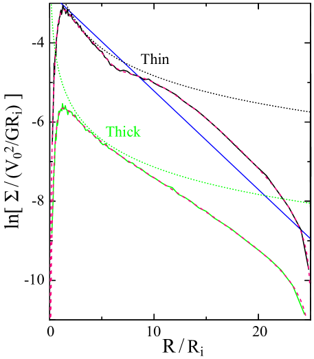
Figure 1: Initial surface density profiles of the tapered thin (top black curves) and thick (bottom green curves) Mestel discs in simulation M2 (solid curves) measured from the particles. The dashed red curves, which are almost perfectly overlaid by the solid curves, show the expected surface density of the tapered discs from integrating the DF over all velocities, while the dotted curves indicate the density profiles of the corresponding non-tapered discs. The groove in the thin disc is centred on $R=6.5R_{i}$ and is broadened by epicycle excursions. The blue line of slope $-0.25$ indicates the adopted exponential profile of the thin disc.

We thicken these disc models by giving each the scaled vertical density profile

$$\rho(\tilde{z})\propto\frac{1}{\left(e^{|\tilde{z}|/2}+0.2e^{-5|\tilde{z}|/2}\right)^{2}},$$ (5)

where $\tilde{z}=z/z_{0}$ with $z_{0}$ independent of $R$. While both this function and the usual $\hbox{sech}^{2}z$ function have harmonic cores, we prefer eq. (5) because it approaches $\rho\propto e^{-|\tilde{z}|}$ more rapidly, as suggested by data (e.g. Kregel, van der Kruit & de Grijs, 2002); $z_{0}$ is therefore the exponential scale height when $z\gg z_{0}$. We set the vertical scale height of the thick disc to be three times that of the thin disc, as suggested for the Milky Way (Jurić et al., 2008).

We estimate the equilibrium vertical velocity dispersion at each $z$-height by integrating the 1D Jeans equation (BT08, eq. 4.271) in our numerically-determined potential. This procedure is adequate when the radial velocity dispersion is low, but the vertical balance degrades in populations having larger initial radial motions, which flare outwards as the model relaxes from initial conditions, as shown below.

The tapered thin Mestel disc has a surface density that declines with radius as shown in Fig. 1. While there is no radial range that is closely exponential, we estimate an approximately equivalent exponential radial scale length $R_{d}=4.0R_{i}$ as shown by the blue line. Accordingly, we choose $z_{0}=0.4R_{i}$ for the thin disc so that the ratio $R_{d}/z_{0}$ is similar to that of the Milky Way and the average volume-corrected ratio of $7.3\pm 2.2$($1\sigma$) found by Kregel, van der Kruit & de Grijs (2002) for 34 nearby galaxies. The values we adopt for each model are given in Table 1 below.

The radial gravitational potential gradient in the midplane of our model is less than that of the full-mass, razor-thin, infinite Mestel disc as a result of the reduced disc surface density, the angular momentum tapers, the finite thickness of the discs, and gravitational force softening. In order to create an approximate equilibrium, we therefore add a rigid central attraction to the self-consistent forces from the particles in the discs at each step. We tabulate the supplementary central attraction needed at the initial moment to yield a radial force per unit mass of $-V_{0}^{2}/R$ in the midplane, and apply this unchanging extra term as a spherically symmetric, rigid central attraction.

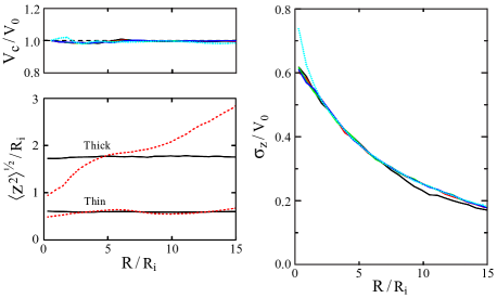
Figure 2: The circular velocity in disc midplane (top left) and vertical velocity dispersion of the thick disc particles (right) at five equally spaced times during simulation M2. The times, which include the initial and final moments of the simulation, are colour coded in temporal order by solid black, red, green, blue, and dotted cyan respectively. The dashed horizontal line in the top left panel shows the theoretical circular velocity $V_{0}=1$. The bottom left panel shows the initial $\left\langle z^{2}\right\rangle^{1/2}$ of the thin (bottom curves) and thick (top curves) discs (solid black) compared to that at $t=32R_{i}/V_{0}$ (dashed red).

Table 1: Parameters of all the simulations described in this paper.

Simulation	Disc	$f$	$\frac{z_{0}}{R_{i}}$	$\frac{\sigma_{R}}{V_{0}}$	$N$	$m$	$\frac{\Delta z}{R_{i}}$	$\frac{\varepsilon}{R_{i}}$	Rings$\times$Spokes$\times$Planes
M2	thin	0.5	0.4	0.283	1 200 000	0 , 2	0.1	0.15	120$\times$128$\times$243
	thick	0.05	1.2	0.567	1 800 000
T	thin	0.5	0.4	0.283	1 200 000	0	0.1	0.15	120$\times$128$\times$243
	thick	0.05	1.2	0.567	1 800 000
M3	thin	0.3333	0.4	0.189	1 200 000	0 , 3	0.1	0.15	120$\times$128$\times$243
	thick	0.0333	1.2	0.378	1 800 000
M4	thin	0.25	0.4	0.142	1 200 000	0 , 4	0.1	0.15	120$\times$128$\times$243
	thick	0.025	1.2	0.283	1 800 000
M4b	thin	0.25	0.2	0.142	1 200 000	0 , 4	0.05	0.075	120$\times$128$\times$405
	thick	0.025	0.6	0.283	1 800 000
	massless thick	0	1.2	0.283	1 800 000
M2b	thin	0.5	0.4	0.283	480 000	0 , 2	0.1	0.15	75$\times$80$\times$625
	thick	0.05	1.2	0.567	240 000
	massless 1	0	0.5	0.567	240 000
	massless 2	0	0.6	0.567	240 000
	massless 3	0	0.7	0.567	240 000
	massless 4	0	0.8	0.567	240 000
	massless 5	0	1.6	0.567	240 000
	massless 6	0	2.0	0.567	240 000
	massless 7	0	2.4	0.567	240 000
M2c	thin	0.5	0.4	0.283	480 000	0 , 2	0.1	0.15	75$\times$80$\times$243
	thick	0.05	1.2	0.567	240 000
	massless 1	0	1.2	0.378	240 000
	massless 2	0	1.2	0.454	240 000
	massless 3	0	1.2	0.680	240 000
	massless 4	0	1.2	0.794	240 000
	massless 5	0	1.2	0.907	240 000
	massless 6	0	1.2	1.021	240 000
	massless 7	0	1.2	1.134	240 000
TK	thick	0.5	1.2	0.283	1 800 000	0 , 2	0.1	0.15	120$\times$128$\times$243
UC , UCB1,	thin	0.4	0.4	0.227	200 000	$\leq$ 8, $\neq$ 1	0.2	0.3	75$\times$80$\times$125
UCB2	thick	0.04	1.2	0.454	300 000

The first column gives the simulation designation used in the text. The next five columns give the properties of each disc, one for each line: $f$ is the mass fraction, $z_{0}$ its vertical scale height, $\sigma_{R}$ is the nominal radial velocity dispersion, and $N$ is the number of particles in the disc. The final four columns give $m$, the active sectoral harmonic(s), $\Delta z$ the vertical spacing of the grid planes, $\varepsilon$ the softening length, and the grid size. The “massless” discs of simulations M4b, M2b, and M2c describe massless thick discs composed of test particles. $z_{0}$, $\Delta z$, and $\varepsilon$ are in terms of $R_{i}$, and $\sigma_{R}$ is in terms of the circular velocity $V_{0}$.

We find that our model is close to equilibrium, with an initial virial ratio of the particles of $\approx 0.52$. This value adjusts quickly to reach a steady virial ratio of $0.50$ within the first 32 dynamical times (defined below). As noted above, the initial imbalance seems to arise mostly from the vertical velocity structure, for which we adopted the 1D Jeans equation. The adjustment of the model to equilibrium is illustrated in Fig. 2; the bottom left panel shows that thicknesses of both discs change as the system relaxes, increasing in the outer parts and decreasing in the inner parts – notice that the change in thickness is least over the radius range $2R_{i}\la R\la 10R_{i}$, where the surface mass density is closest to its untapered value (dotted curves in Fig. 1). The changes, which are larger for the radially-hotter thick disc, result from the radial excursions of the particles, which may take them far from their initial radii for which the vertical velocity was set. However, neither the radial balance (top left panel) nor the vertical velocity dispersion (right panel) of the thick disc change significantly from their initial values. After this initial relaxation from initial conditions, we do not observe any significant flaring. A negligibly small fraction ($<1\%$) of particles escape from our grid by the end of the simulation, and most particle loss takes place as the model settles.

Following Sellwood & Binney (2002), we seed a vigorously unstable spiral mode by adding a Lorentzian groove in angular momentum to the DF of the thin disc only:

$$f(E,L_{z})=f_{0}(E,L_{z})\left[1+\frac{\beta w_{L}^{2}}{(L_{z}-L_{*})^{2}+w_{L}^{2}}\right].$$ (6)

Here $\beta$, a negative quantity, is the depth of the groove, $w_{L}$ is its width, and $L_{*}$ is the angular momentum of the groove centre. This change to the DF seeds a predictable spiral instability (Sellwood & Kahn, 1991). The groove in the thin disc has the parameters $\beta=-0.9$, $w_{L}=0.3R_{i}V_{0}$, and $L_{*}=6.5R_{i}V_{0}$. We find that a deeper and wider groove is needed than that used by Sellwood & Binney (2002) in order to excite a strong spiral in our thickened disc.

Since a groove of this kind will provoke instabilities at many sectoral harmonics, $m$, we restrict disturbance forces from the particles to a single non-axisymmetric sectoral harmonic to prevent other modes from growing. Corotation for a global spiral mode excited by this groove is at a radius somewhat greater than $L_{*}/V_{0}$, where local theory would predict. A large-scale mode is not symmetric about the groove centre due to the geometric variation of surface area with radius – an effect that is neglected in local theory. However, the radius of corotation approaches the local theory prediction for modes of smaller spatial scale, i.e. as $m\rightarrow\infty$.

As in Sellwood & Binney (2002), we choose the circular velocity $V_{0}$ to be our unit of velocity, $R_{i}$ our unit of length, the time unit or dynamical time is $\tau_{0}=R_{i}/V_{0}$, our mass unit is $M_{0}=V_{0}^{2}R_{i}/G$, and $L_{i}$ is our unit of angular momentum. One possible scaling to physical units is to choose $R_{i}=0.75\;$kpc, with $R_{d}=4.0R_{i}$ being the equivalent scale length of the thin disc, and $\tau_{0}=3.0\;$Myr, leading to $V_{0}=244\;$km s^-1 and $M_{0}=1.04\times 10^{10}\;$M_⊙.

2.2 Numerical procedure

We use the 3D polar grid described in Sellwood & Valluri (1997) to determine the gravitational field of the particles. This “old-fashioned” method is not only well suited to the problem, but also has the advantage of being tens of times faster than the “modern” methods recently reviewed by Dehnen & Read (2011). We employ a grid having $120$ rings, $128$ spokes, and $243$ vertical planes, and adopt the cubic spline softening rule recommended by Monaghan (1992), which yields the full attraction of a point mass at distances greater than two softening lengths ($2\varepsilon$). The Plummer rule used in Sellwood & Binney (2002) is suited for razor-thin discs where it mimics the effect of disc thickness but, because it weakens inter-particle forces on all scales, it is unsuited for 3D simulations where disc thickness is already included in the particle distribution. The value of $\varepsilon$, given in Table 1, exceeds the vertical grid spacing in order to minimize the grid dependence of the inter-particle forces.

In the simulations described in §§3&4, we use quiet starts (Sellwood & Athanassoula, 1986) for both discs to reduce the initial amplitude of the seeded unstable spiral mode far below that expected from shot noise. In 3D, this requires many image particles for each fundamental particle: we place two at each $(R,\phi,z)$ position with oppositely directed $z$-velocities and two more reflected about the midplane at the point $(R,\phi,-z)$. We then place images of these four particles at equal intervals in $\phi$, each set having identical velocity components in cylindrical polar coordinates. For these simulations, the thin disc has $1\,200\,000$ particles and the thick disc $1\,800\,000$. All the particles in a single population have equal mass, but particle masses differ between populations in order to create the desired ratio of disc surface densities.

We evaluate forces from the particles at intervals of $0.02\tau_{0}$, and step forward some of the particles at each evaluation. Since the orbital periods of particles span a wide range, we integrate their motion when $R>2R_{i}$ using longer time steps in a series of five zones with the step doubling in length for each factor 2 in radius (Sellwood, 1985). We also subdivide the time step for particles within $R=0.5R_{i}$ without updating forces, with further decreases by a factor of $2$ for every factor of $2$ decrease in radius (Shen & Sellwood, 2004). Note that very few particles have $R<0.5R_{i}$, which is well within the inner taper where the rigid component of the force dominates. Tests with shorter time steps yielded similar results.

2.3 List of simulations

For convenience, we summarize the parameters of all the simulations presented in this paper in Table 1. Simulation T is constrained to remain axisymmetric, while all those whose identifier begins with ‘M’ are highly controlled experiments designed to support a single spiral instability. We first present, in §3, a detailed description of M2, which supports a bisymmetric spiral, and briefly compare it to simulation T. Variants of M2, with many populations of test particles are presented in §3.4, while simulation TK, which has a thick disc only, is described in §3.5. Simulations that support a single spiral of higher angular periodicity are motivated and described in §4. The last three simulations in the Table, with identifier beginning with ‘U’, are uncontrolled experiments presented in §5 that explore the consequences of multiple spirals, with and without a bar.

3 A single bisymmetric spiral

Our first objective is to study radial migration in both the thick and thin discs due to a single spiral disturbance. We therefore present simulation M2, which is designed to support an isolated $m=2$ spiral instability.

We measure

$$A_{m}(t)=2\pi\int_{R_{1}}^{R_{2}}\Sigma(R,\phi,t)e^{im\phi}\;dR,$$ (7)

where $\Sigma(R,\phi,t)$ is the vertically-integrated mass surface density of the particles at time $t$, and we generally choose $R_{1}=1.5R_{i}$ and $R_{2}=19R_{i}$.

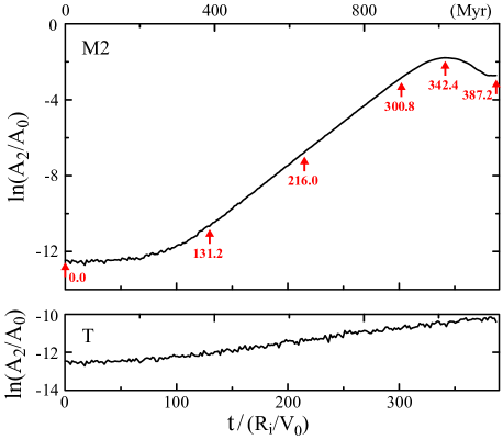
Figure 3: The time evolution of $A_{2}/A_{0}$ in simulations M2 (top) and T (bottom). Note the difference in the vertical scales. The numbered arrows in the top plot mark the six times of M2 at which the snapshots of the discs are shown in Fig. 4. The top axis shows time scaled to physical units using the adopted scaling at the end of section 2.1.

The top panel of Fig. 3 shows the time evolution of $A_{2}/A_{0}$, revealing that the mode grows exponentially, peaks, and then decays non-exponentially to a trough. The peak is $2.55$ times higher than the minimum of the following trough. Continued evolution reveals that the amplitude rises again due to the growth of a secondary wave. In order to isolate the single initial spiral, we stop the simulation at the trough and compare quantities, such as the specific angular momenta of particles, at this final time with those at the initial time $t=0.0R_{i}/V_{0}$. The bottom panel plots the same quantity from simulation T in which disturbance forces from the particles were restricted to the axisymmetric ($m=0$) term; the very slow rise is caused by the gradual degradation of the quiet start.

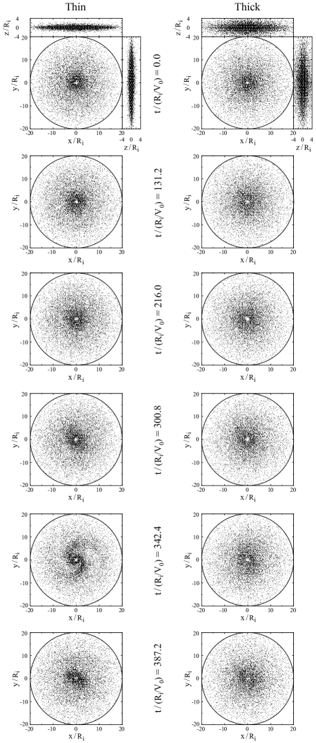
Figure 4: Snapshots of the thin (left column) and thick (right column) discs in simulation M2 at the six times marked in Fig. 3. One in every $24$ particles is plotted for the thin disc, and one in every $36$ for the thick. The side views are shown only at the initial time because they change little throughout the simulation.

Fig. 4 shows snapshots of the thin and thick discs of M2 at six different times of the simulation that are marked by the red arrows in Fig. 3.

We find the period of exponential growth can be very well fitted by a single mode, using the apparatus described in Sellwood & Athanassoula (1986). Table 2 reports the fitted pattern speed $\Omega_{p}$ and growth rate $\gamma$, together with other parameters of the spiral in M2. Furthermore, the non-linear evolution visible in Fig. 4 shows no evidence of a bar. Thus, the selected time period of the simulation M2 presents the opportunity to study radial migration due to a single, well isolated spiral wave. Note that the spiral pattern makes a full rotation every $2\pi/\Omega_{p}\simeq 45.5R_{i}/V_{0}$.

Table 2: Measured values from fits to the spiral modes.

	$m$	$\Omega_{p}/\frac{V_{0}}{R_{i}}$	$\gamma$	$\frac{R_{c}}{R_{i}}$	$\left(\frac{A_{m}}{A_{0}}\right)_{\rm peak}$	P/T	$t_{p}/\frac{R_{i}}{V_{0}}$ , ($Myr$)
M2	2	0.138	0.0454	7.24	0.168	2.55	73.5 , 221
M3	3	0.147	0.0417	6.81	0.099	2.15	76.9 , 231
M4	4	0.150	0.0361	6.67	0.063	1.80	76.3 , 229
M4b	4	0.151	0.0465	6.63	0.083	3.07	81.3 , 244
M2b	2	0.138	0.0457	7.25	0.166	2.52	72.1 , 216
M2c	2	0.138	0.0456	7.25	0.166	2.52	74.4 , 223
TK	2	0.135	0.0180	7.40	0.064	1.68	149 , 446

The second column gives the angular periodicity of the spiral or the greatest active sectoral harmonic $m$ in the simulation. The next three columns give the pattern speed $\Omega_{p}$, growth rate $\gamma$, and the corotation radius $R_{c}$ of the spiral obtained by fitting it’s exponential growth using the method in Sellwood & Athanassoula (1986). The next two columns provide the spiral’s peak amplitude and $\left(\frac{A_{m}}{A_{0}}\right)_{\rm peak}/\left(\frac{A_{m}}{A_{0}}\right)_{\rm trough}$. And the last column gives the duration of the peak amplitude, which we measure between the moment the amplitude reaches the trough and the moment preceding the peak at which the amplitude is at the same level as the trough amplitude. The second number in the peak duration column is the time in physical units using the adopted scaling at the end of section 2.1.

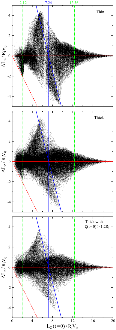
Figure 5: Angular momentum changes of particles in M2 as a function of their initial angular momenta. The top panel is for thin disc particles, the middle for all thick disc particles, and the bottom for thick disc particles having notional vertical amplitude $\zeta>1.2R_{i}$. The horizontal red line denotes zero change. The vertical lines mark the Lindblad resonances (dashed green) and corotation (solid blue). The solid blue line with a slope of $-2$ illustrates the locus of particles whose changes would be symmetric about corotation. The dashed red line of slope $-1$ shows the $\Delta L_{z}=-L_{z}(t=0)$ locus below which particles end up on retrograde orbits.

3.1 Angular momentum changes

Fig. 5 shows the change in the specific $z$-angular momenta $\Delta L_{z}$ of the particles in the thin disc (top) and the thick disc (middle) of simulation M2 against their initial $L_{z}$. The deficiency of particles at $L_{z}(t=0)=L_{*}=6.5R_{i}V_{0}$ in the top panel is due to the groove in the thin disc. The vertical lines show the locations of the corotation (solid blue) and the Lindblad resonances (dashed green) for nearly circular orbits.

The maximum changes in angular momentum occur near corotation, and lie close to the solid blues line of slope $-2$; these particles cross corotation, in both directions, to about the same radial distance away from it as they were initially. As for the razor-thin disc, we find that large angular momentum changes occur only around the time that the spiral saturates, for reasons explained by Sellwood & Binney (2002). While many particles near the inner Lindblad resonance lose angular momentum, only a tiny fraction end up on retrograde orbits. Note also that $\left\langle(\Delta L_{z})^{2}\right\rangle^{1/2}\approx 9.0\times 10^{-6}R_{i}V_{0}$ in simulation T, where non-axisymmetric forces were eliminated, showing that changes in $L_{z}$ due to orbit integration and noise errors are tiny in comparison to those caused by the spiral.

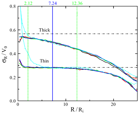
Figure 6: The radial variations of $\sigma_{R}$ in the thin (bottom curves) and thick (top curves) discs of M2 at the same five different times as used in the top left and right panels of Fig. 2 with the same line colour and style coding. The horizontal dot-dashed curves show the theoretical initial dispersions from the untapered discs, while the vertical lines mark the principal resonances of the spiral, colour and style coded as in Fig. 5.

For each particle, we determine the initial value of

$$Z=\frac{1}{2}v_{z}^{2}+\frac{1}{2}\nu^{2}z^{2},$$ (8)

where $v_{z}$ is the vertical velocity component at distance $z$ from the midplane and $\nu$ is the vertical frequency measured in the midplane at the particle’s initial radius $R$. For particles whose vertical and radial oscillations are small enough to satisfy the epicycle approximation, $Z=E_{z,\rm epi}$ the energy of its vertical oscillation; the vertical potential is roughly harmonic for $|z|\la 0.4R_{i}$. Even though the epicycle approximation is not satisfied for the majority of particles, we compute an initial notional vertical amplitude

$$\zeta=\left(\frac{2Z}{\nu^{2}}\right)^{1/2},$$ (9)

for them all. The value of $\zeta$ defined in this way, i.e. at the initial moment only, yields a convenient approximate ranking of the vertical oscillation amplitudes of the particles, although it is clear that in most cases $\zeta<z_{\rm max}$, the maximum height a particle may reach. Note that since each disc component in our models has an initial thickness that is independent of radius, the distribution of $\zeta$ is independent of $L_{z}(t=0)$.

Notice from Fig. 5 that changes for the thick disc particles are only slightly smaller than those for thin disc particles. In order to emphasize this point, the bottom panel displays only those thick disc particles for which $\zeta>1.2R_{i}$, or one scale height of the thick disc, revealing that even for these particles changes can be almost as large as those in the thin disc.

Fig. 6 shows the evolution of the radial velocity dispersion for the thin and thick discs. As expected (Sellwood & Binney, 2002), the large angular momentum changes near corotation cause little heating. Some heating occurs near the Lindblad resonances, and is greater near the inner resonance, again as expected.

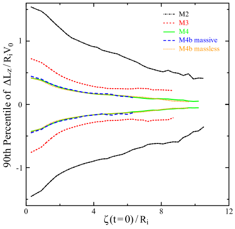
Figure 7: The 5th and 95th percentiles of the angular momentum changes in the thick discs of simulations M2 (dot-dashed black), M3 (short-dashed red), M4 (solid green), the massive thick disc of M4b (long-dashed blue), and the massless thick disc of M4b (dotted orange) as a function of notional vertical amplitude $\zeta$. Although we have smoothed the curves, the rising noise with increasing $\zeta$ is caused by the decrease in the number of particles per bin. The curves stop when the number of particles per bin drops below twenty.

3.2 Distribution of angular momentum change

Table 3 lists the root mean square, maximum positive, and maximum negative changes in angular momentum for both all the particles and only those that satisfy $\zeta>z_{0}$ in each disc.

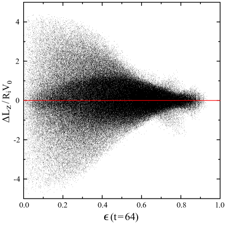
Figure 8: Angular momentum changes of thick disc particles between the final time and $t=64R_{i}/V_{0}$ having $2.5R_{i}V_{0}\leq L_{z}(t=64)\leq 10.0R_{i}V_{0}$ in simulation M2 as a function of their eccentricities at $t=64R_{i}/V_{0}$. The plot for the thin disc is quite similar. The red horizontal line shows zero angular momentum change.

Table 3: Changes in angular momentum resulting from the spirals and bar.

	Disc	$\frac{\left\langle(\Delta L_{z})^{2}\right\rangle^{1/2}}{R_{i}V_{0}}$	$\frac{\textrm{Max }\Delta L_{z}}{R_{i}V_{0}}$	$\frac{\textrm{Max -}\Delta L_{z}}{R_{i}V_{0}}$
M2	thin	1.59 , 1.56	4.44 , 4.37	-4.83 , -4.79
	thick	0.97 , 0.85	4.38 , 3.91	-4.78 , -4.46
M3	thin	0.92 , 0.89	2.79 , 2.72	-2.67 , -2.61
	thick	0.54 , 0.43	2.76 , 2.22	-2.60 , -2.12
M4	thin	0.62 , 0.60	2.03 , 1.97	-2.11 , -2.02
	thick	0.37 , 0.30	1.93 , 1.65	-1.99 , -1.59
M4b	thin	0.80 , 0.78	2.25 , 2.18	-2.17 , -2.08
	thick	0.47 , 0.40	2.21 , 1.84	-2.09 , -1.83
	massless	0.38 , 0.27	2.17 , 1.43	-2.05 , -1.48
M2b	thin	1.58 , 1.54	4.45 , 4.36	-4.57 , -4.43
	thick	0.95 , 0.84	4.33 , 3.76	-4.52 , -4.02
	massless 1	1.08 , 1.06	4.42 , 4.32	-4.43 , -4.43
	massless 2	1.06 , 1.02	4.41 , 4.19	-4.54 , -4.22
	massless 3	1.04 , 0.98	4.41 , 4.08	-4.47 , -4.27
	massless 4	1.02 , 0.95	4.48 , 4.11	-4.43 , -4.15
	massless 5	0.89 , 0.72	4.35 , 3.46	-4.40 , -3.67
	massless 6	0.83 , 0.64	4.39 , 3.11	-4.29 , -3.64
	massless 7	0.79 , 0.58	4.05 , 3.06	-4.30 , -3.37
M2c	thin	1.57 , 1.53	4.46 , 4.35	-4.58 , -4.44
	thick	0.96 , 0.85	4.33 , 3.76	-4.50 , -4.03
	massless 1	1.19 , 1.06	4.37 , 3.75	-4.42 , -4.11
	massless 2	1.08 , 0.95	4.37 , 3.81	-4.46 , -4.01
	massless 3	0.86 , 0.76	4.37 , 3.66	-4.49 , -4.09
	massless 4	0.80 , 0.72	4.35 , 3.70	-4.28 , -4.09
	massless 5	0.75 , 0.68	4.22 , 3.79	-4.33 , -3.89
	massless 6	0.72 , 0.65	4.18 , 3.56	-4.51 , -3.81
	massless 7	0.69 , 0.63	4.21 , 3.51	-4.29 , -3.81
TK	thick	0.78 , 0.75	3.37 , 3.26	-2.88 , -2.77
UC	thin	2.65 , 2.31	13.97 , 11.60	-10.43 , -9.48
	thick	1.95 , 1.75	12.71 , 10.33	-10.15 , -10.04
UCB1	thin	3.15 , 2.76	16.42 , 12.41	-13.22 , -11.12
	thick	2.34 , 2.10	16.00 , 13.80	-12.00 , -10.92
UCB2	thin	3.53 , 3.46	19.23 , 19.14	-16.74 , -16.74
	thick	2.54 , 2.28	19.31 , 17.40	-15.83 , -13.63

For each disc of every simulation, the first numbers in the third, fourth, and fifth columns give the root mean square, maximum positive, and maximum negative changes in angular momentum respectively. We calculate these for all the particles except those that escaped the grid for which the initial angular momentum lies in an interval of the spiral’s main influence around its corotation. This interval, in values in terms of $R_{i}V_{0}$, is $[2.5,10]$ for simulations M2, M2b, and M2c, $[4.5,9.5]$ for M3, $[5.0,8.5]$ for M4 and M4b, and $[3.5,9.5]$ for TK. We do not confine $L_{z}(t=0)$ to such an interval for simulations UC, UCB1, and UCB2 since the influence of their spirals and bar span almost the entire range. The second numbers in the last three columns give the same results but only for particles having notional vertical amplitude $\zeta>z_{0}$.

Fig. 7 shows the 5th and 95th percentile values of the changes in angular momentum as a function of initial notional vertical amplitude, $\zeta$ (eq. 9), using bin widths of $0.3R_{i}$. The affect of radial migration seems to decrease almost linearly with increasing $\zeta$.

Radial migration should also be weaker for particles having larger radial oscillations or epicycles of large amplitude. As reasoned by Sellwood & Binney (2002), particles on more eccentric orbits cannot hold station with a steadily rotating spiral, because their angular velocities vary significantly as they oscillate radially. Fig. 8, which is for only those particles in the angular momentum range $2.5R_{i}V_{0}\leq L_{z}(t=64)\leq 10.0R_{i}V_{0}$, confirms that the largest angular momentum changes occur among particles having the least eccentric orbits. It shows angular momentum changes from, and eccentricities at, time $t=64R_{i}/V_{0}$, which is after the model has settled from its mild initial imbalance, but before any substantial angular momentum changes have occurred. We define eccentricity as $\epsilon=(R_{\rm a}-R_{\rm p})/(R_{\rm a}+R_{\rm p})$, in which $R_{\rm a}$ and $R_{\rm p}$ are respectively the initial apo-centre and peri-centre distance of the orbit of a particle having the same $L_{z}$, but whose motion is confined to the midplane of the axisymmetric potential.

3.3 Effect of radial migration on vertical oscillations

In the previous subsection, we showed how the particles’ angular momentum changes vary with initial amplitude of vertical motion. Here, we present the converse: how the vertical oscillations are affected by the radial excursions.

Since the notional amplitude of vertical motion $\zeta$ (eq. 9) is accurate only in the epicycle approximation, we determine a particle’s actual maximum vertical excursion, $z_{\rm max}$, by integrating its motion in a frozen, azimuthally-averaged potential for many radial periods. We do this twice for each particle in simulation M2, at time $t=64R_{i}/V_{0}$ starting from the particle’s phase space coordinates in the frozen potential at that moment and again at the final time $t=387.2R_{i}/V_{0}$.

Fig. 9 shows that, on average, the vertical excursions of particles increase for those that move radially outwards and decrease for those that move inwards. This is expected, because restoring forces to the mid-plane are weaker at larger radii. For both discs, the mean (solid green) and median (dashed blue) curves show a roughly constant $\Delta z_{\rm max}$ for a wide range of $\Delta L_{z}$. For the thick disc, this constant $\Delta z_{\rm max}$ is about twice as great as that for the thin.

While the large majority of the particles lie in the contoured region, the outliers exhibit significant substructure. The dense group of points near a line of slope of $-1$ in the second quadrant are particles with initial home radii within and near the inner $m=2$ vertical resonance, which lies at the radius $2.23R_{i}$, not far from the radial inner Lindblad resonance at $2.12R_{i}$. Usually $\nu\gg\kappa$, which causes vertical resonances to be found significantly farther from corotation than the radial resonances, but in our case the inner taper reduces the inner surface density so that $\nu\sim\kappa$ in this part of the disc. Thus, these particles are scattered vertically at the inner vertical resonance at the same time as they lose angular momentum at the radial inner Lindblad resonance. Another outlying group can be seen in the first quadrant, with large $\Delta z_{\rm max}$ for small $\Delta L_{z}$; these particles have quite eccentric initial orbits that have particular radial phases just before the spiral saturates. Either they are at their pericentres and lie near corotation just trailing either spiral arm, or they are at their apocentres and surround the outer ends of the spiral arms. Being at these special locations when the spiral wave is strongest, gives them instantaneous angular frequencies about the centre that cause them to experience more nearly steady, and not oscillatory, torques from the perturbation, leading to some angular momentum gain. Thus these particles move onto even more eccentric orbits and their increased $z_{\rm max}$ occurs at their new larger apocentres.

Figure 9: Changes in maximum vertical excursions of particles in the thin (top) and thick (bottom) discs of M2 versus changes in their angular momenta. Contours are linearly spaced in number density and we plot only those points that lie outside the lowest contour. The mean (solid green) and median (dashed blue) show systematic variations, as expected. Note that the vertical scales differ in the two plots.

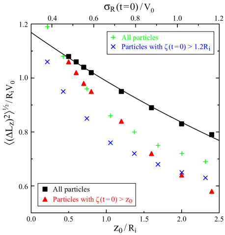
Figure 10: The filled symbols show $\left\langle(\Delta L_{z})^{2}\right\rangle^{1/2}$ as a function of vertical thickness (bottom axis) of particle populations of simulation M2b. The black squares are for all the particles in the angular momentum range $2.5R_{i}V_{0}\leq L_{z}(t=0)\leq 10.0R_{i}V_{0}$, while the red triangles are for only those particles having $\zeta>z_{0}$. The line is a least-squares fit to the black squares of the form $\left\langle(\Delta L_{z})^{2}\right\rangle^{1/2}\propto e^{-z_{0}/5.95R_{i}}$. The green plus symbols show the variation of $\left\langle(\Delta L_{z})^{2}\right\rangle^{1/2}$ with initial radial velocity dispersion (top axis) of all the particles in the same $L_{z}(t=0)$ range from populations in simulation M2c. The blue crosses are for only those with $\zeta>z_{0}=1.2R_{i}$.

3.4 Effects of disc thickness and radial velocity dispersion

Our somewhat surprising finding from simulation M2 is that angular momentum changes in the thick disc are only slightly smaller than those in the thin, and also in the razor-thin disc of (Sellwood & Binney, 2002). Despite the fact that thick disc particles both rise to greater $z$ heights and have larger epicycles, on average, than do thin disc particles, we observe only a mild decrease in their response to spiral forcing. This finding suggests that the potential variations of a spiral having a large spatial scale, such as the $m=2$ spiral mode in simulation M2, couple well to particles having large vertical motions and epicycle sizes.

To provide more detailed information about how the extent of angular momentum changes vary with disc thickness, we added seven test particle populations to some simulations. In M2b, all test particle populations have the same initial radial velocity dispersion as the massive thick discs, but have scale heights in the range $0.5R_{i}\leq z_{0}\leq 2.4R_{i}$. Simulation, M2c, employs seven test particle populations having the same scale height ($z_{0}=1.2R_{i}$) as the massive thick disc, but with differing $\sigma_{R}$.

Being test particles, they do not affect the dynamics of the spiral instability, but merely respond to the potential variations that arise from the instability in the massive components. These simulations have identically the same physical properties as M2 but lower numerical resolution as summarized in Table 1; the reduced numerical resolution remains adequate since the fitted spiral mode is little changed from that in simulation M2 (Table 2).

Variations of $\left\langle(\Delta L_{z})^{2}\right\rangle^{1/2}$ with both disc thickness, at fixed radial velocity dispersion, and of radial dispersion at fixed thickness, are displayed in Fig. 10. The decrease is somewhat more rapid in subpopulations of particles that start with a notional vertical amplitude $\zeta>z_{0}$, as seems reasonable. The fitted line indicates that $\left\langle(\Delta L_{z})^{2}\right\rangle^{1/2}$ decays approximately exponentially with disc thickness with a scale that can be related to theory – see §4.3. Table 3 gives both the plotted root mean square, as well as the maximum positive, and maximum negative $\Delta L_{z}$ for all the particles of each population and separately for those with $\zeta>z_{0}$ of each disc.

We caution that the information in Table 3 and in Fig. 10 quantifies how the responsiveness of a test particle population scales when subject to a fixed perturbation. Self-consistent spiral perturbations may differ in strength, spatial scale, and/or time dependence causing quite different angular momentum changes.

3.5 Thick disc only

For completeness, we also present simulation TK, which has a single, half-mass active disc with a substantial thickness. We inserted the same initial groove, and restricted forces to $m=2$ only.

It is interesting that a groove in the thick disc still creates a spiral instability, but one that grows less rapidly and saturates at a lower amplitude than we found in M2. As a consequence, the spread in $\left\langle(\Delta L_{z})^{2}\right\rangle^{1/2}$ is about $1/2$ as large as in M2. Again we find that the radial migration is reduced by increasing disc thickness, but not inhibited entirely.

4 Other simulations

The potential of a plane wave disturbance in a thin sheet having a sinusoidal variation of surface density $\Sigma_{a}$ in the $x$-direction is

$$\Phi_{a}(x,z)=-{2\pi G\Sigma_{a}\over|k|}e^{ikx}e^{-|kz|}$$ (10)

where $k$ is the wavenumber (BT08, eq. 5.161). The exponential decay away from the disc plane is steeper for waves of smaller spatial scale, i.e. larger $|k|$. While spirals are not simple plane waves in a razor-thin sheet, this formula suggests that we should expect radial migration to be weakened more by disc thickness for spirals of smaller spatial scale or higher angular periodicity – note that the azimuthal wavenumber, $k_{\phi}=m/R$. The simulations in this section study the effect of changing this parameter.

4.1 Spirals of different angular periodicities

We wish to create spiral disturbances that are similar to that in M2, but have higher angular periodicities. Since we expect migration to depend not only on the spatial scale relative to the disc thickness, but also the peak amplitude, $\Sigma_{a}$, and perhaps also the time dependence, we try to keep as many factors unchanged as possible.

The mechanics of the instability seeded by a groove depends strongly on the supporting response of the surrounding disc (Sellwood & Kahn, 1991), which in turn, according to local theory, depends on the vigour of the swing amplifier (Toomre, 1981). Thus to generate a similar spiral disturbance with $m>2$, we need to hold the key parameters $X$ and $Q$ at similar values. For an $m$-armed disturbance in a thin, single component Mestel disc with active mass fraction $f$, the locally-defined parameter

$$X=\frac{2}{fm}$$ (11)

is independent of radius. We therefore scale the active mass fractions in both components as $f\propto m^{-1}$ – recall that we used a half-mass disc for $m=2$. In order to preserve the same $Q$ value (eq. 3), the radial velocity dispersion of the particles also has to be reduced as $\sigma_{R}\propto f$.

Simulations M3 and M4 therefore have lower surface densities and smaller velocity dispersions in order to support similarly growing spiral modes of sectoral harmonic $m=3$ and 4 respectively. A further simulation M4b is described below. These models are all seeded with a groove of the same form (eq. 6) and parameters as that in M2.

Note that the instability typically extends between the Lindblad resonances, which move closer to corotation as $m$ is increased. In the Mestel disc, the radial extent of the mode varies as

$$\frac{R_{\rm OLR}}{R_{\rm ILR}}=\frac{m+\sqrt{2}}{m-\sqrt{2}},$$ (12)

i.e. $R_{\rm OLR}/R_{\rm ILR}\approx 5.8$, 2.8 & 2.1, for $m=2$, 3 & 4 respectively. Since we have also decreased the in-plane random motion in proportion to the surface density decrease, the decreased size of the in-plane epicycles somewhat compensates for the smaller scale of the mode, although the ratio is not exactly preserved.

4.2 Results for $m>2$

Table 2 gives our estimates of the spiral properties in each simulation; uncertainties in the measured frequencies are typically $\la 2\%$ (Sellwood & Athanassoula, 1986). The pattern speeds of these instabilities do not change much with $m$, except that we find the radius of corotation lies closer to the groove centre $L_{*}/V_{0}=6.5R_{i}$, as expected. The table also gives the time during which the amplitude of the wave is equal to or greater than that at the post-peak trough, which again does not vary much with angular periodicity. However, both the growth rates and the peak amplitudes of the modes decrease from M2, to M3 and M4.

Table 3 includes the root mean square, maximum positive, and maximum negative angular momentum changes for M3, M4, and M4b, measured in each case to the moment at which $A_{m}$ passes through the first minimum after the mode has saturated. Comparison with M2 reveals that increasing $m$ causes a roughly proportionate decrease in the angular momentum changes, in part because the saturation amplitude is lower, but perhaps also because the spatial scale is reduced. Note that again some thick disc particles in both M3 and M4 have $\Delta L_{z}$ values almost as large as the greatest in the thin disc, as was also the case for M2.

Fig. 7 shows 5th and 95th percentile values of $\Delta L_{z}$ versus initial notional vertical amplitude $\zeta$ for simulations M3, M4, and M4b. Compared to the curve of M2, the $\Delta L_{z}$ values are smaller for greater $m$ – i.e. the extent of radial mixing is substantially lessened. Note that this difference could have a variety of causes, such as the lower limiting amplitude of the mode, or possibly the different growth rate of the mode, and/or the different disc thickness relative to the spatial scale of the mode.

This last factor is one we are able to eliminate. The thickness of the discs of simulations M2, M3, and M4 were held fixed as we increased $m$ and reduced the surface density. In order to eliminate a change in the ratio of disc thickness to spatial scale of the mode, we ran a further simulation M4b with the same in-plane parameters as in M4, but with half the disc thickness. We also halved the gravity softening length and the vertical spacing of the grid planes.

This change restores the growth-rate of the mode in run M4b to a value quite comparable to that in simulation M2 (Table 2). The saturation amplitude, while larger than in simulation M4, is still about half that in M2. In addition, we added a test particle population to simulation M4b that has parameters identical to those of the massive thick disc, including $\sigma_{R}$ or $q$, except its vertical scale height $z_{0}$ is that of the thick disc of M2, M3, and M4. Again as expected, Table 3 reveals that $\left\langle(\Delta L_{z})^{2}\right\rangle^{1/2}$ is substantially lower in the massless disc than in the thinner, massive disc.

4.3 Comparison with theory

In order to make sense of these results, we here compare with the theoretical picture developed by Sellwood & Binney (2002).

First, we eliminate the possibility that the spiral in the simulations with higher $m$ is “on” for too long for optimal migration. Sellwood & Binney (2002) argue that efficient mixing by the spiral requires the duration of the peak amplitude be less than half the period of a horseshoe orbit, so that each particle experiences only a single scattering. They show that the minimum period of a horseshoe orbit varies as $|\Psi_{0}|^{-1/2}$, where the potential amplitude of the spiral perturbation at corotation varies with the spiral density amplitude, $\Sigma_{a}$, and sectoral harmonic as $|\Psi_{0}|\propto\Sigma_{a}/m$ (eq. 10). Thus the weaker density amplitude that we find with higher $m$ implies that the minimum periods of the horseshoe orbits are greater, and the condition for efficient mixing is more strongly fulfilled for $m>2$.

Theory also suggests that an $m$-dependence of the peak amplitude is unavoidable if the spiral saturates due to the onset of many horseshoe orbits, as was argued in Sellwood & Binney (2002). In their notation, orbits librate – i.e. are horseshoes – when $E_{p}<p^{2}$, where the frequency $p\propto m|\Psi_{0}|^{1/2}$. Since $|\Psi_{0}|\propto\Sigma_{a}/m$ (eq. 10), we see that $p^{2}\propto m\Sigma_{a}$, suggesting that as $m$ increases, horeshoe orbits become important at a lower peak density. Comparing M2 with M4b, we find (Table 2) the relative limiting amplitudes $\Sigma_{a}\propto m^{-1}$, which is consistent with the idea that the spiral instability saturates when the importance of horseshoe orbits reaches very nearly the same level. The fixed thickness and softening length used in M2, M3 and M4 disproportionately weakens the potential of the spiral as $m$ rises, and spoils this exact scaling.

Note also that both $\left\langle(\Delta L_{z})^{2}\right\rangle^{1/2}$ and the extreme values measured from M4b are almost exactly half those in M2, which is also consistent with the horseshoe orbit theory developed by Sellwood & Binney (2002). Since they showed that the maximum $\Delta L_{z}\propto|\Psi_{0}|^{1/2}$, the relations in the previous paragraph require $\Delta L_{z,\rm max}\propto m^{-1}$ as we observe. As the rms value also scales in the same way, it would seem the entire distribution of $\Delta L_{z}$ scales with $m$ in the same way. Again, the constant disc thickness prevents this prediction from working perfectly for M3 and M4.

We stress that this scaling holds because we took some care to ensure the key dynamical properties of the disc were adjusted appropriately. Spirals in a disc having a different responsiveness would have both a different growth rate and probably also peak amplitude, and the behaviour would not have manifested a simple $m$-dependence.

Finally, we motivate the exponential fit to the variation of $\left\langle(\Delta L_{z})^{2}\right\rangle^{1/2}$ with $z_{0}$, for the same $m=2$ spiral disturbance. We have already shown that $\left\langle(\Delta L_{z})^{2}\right\rangle^{1/2}\propto|\Psi_{0}|^{1/2}$, and have argued that the spiral potential decays away from the mid-plane as $e^{-|kz|}$ (eq. 10), with $k_{\phi}=m/R$. Naïvely, we could set $z=z_{0}$, $k=k_{\phi}=m/R$, $m=2$, and $R=R_{c}$, since angular momentum changes are centred on corotation, leading to $\left\langle(\Delta L_{z})^{2}\right\rangle^{1/2}\propto e^{-z_{0}/R_{c}}$. The fitted scale is $5.95R_{i}$, which is somewhat smaller than $R_{c}=7.24R_{i}$. The dominant cause of this discrepancy is probably that spiral is not a plane wave, curvature is important for $m=2$, and that its wavenumber is larger than $k_{\phi}$ because the spiral ridges are inclined to the radial direction; we should therefore expect the potential to decay away from the mid-plane rather more rapidly, in the sense that we measure.

We conclude that angular momentum changes scale with spiral amplitude in the manner predicted in Sellwood & Binney (2002) and, furthermore, the limiting amplitude itself is determined by their theory. The variation with disc thickness is also in the sense expected from the theory, but the quantitative prediction is not exact.

5 Unconstrained Simulations

Having studied at length the effects of a single spiral wave, we now wish to illustrate the effects of multiple spirals. We present three simulations, UC, UCB1, and UCB2, that have no initial groove and the initial positions of the particles are random (i.e. not a quiet start) since we wish spirals to develop quickly from random fluctuations. We include gravitational disturbance forces from all sectoral harmonics $0\leq m\leq 8$, except $m=1$, which we omit in order to avoid imbalanced forces from a possibly asymmetric distribution of particles in a rigid halo with a fixed centre.

All the many simulations of this type that we have run have ultimately developed a strong bar at the centre. We here compare radial migration in three separate cases: simulation UC avoids a bar for a long period and supports many transient spirals, while simulations UCB1 and UCB2 have identical numerical parameters but form a bar quite early. In all three cases, the combined thin and thick discs have a smaller active mass fraction, $f=0.44$, compared with $f=0.55$ for simulation M2. A smaller active mass and a larger gravitational softening length help to delay bar formation but also weaken the $m=2$ spiral amplitudes somewhat. The numerical parameters of these simulations are also listed in Table 1. Since bar formation in these models is stochastic (e.g. Sellwood & Debattista, 2009), the different bar-formation times simply arise from different initial random seeds.

5.1 Multiple spirals only

The black curve in Fig. 11 shows the evolution of $A_{2}/A_{0}$ in simulation UC. The spiral amplitudes rise to the point at which significant particle scattering begins by $t\sim 1\,500R_{i}/V_{0}$ and we present the behaviour up to time $3\,500R_{i}/V_{0}$ shortly before a bar begins to form. The period $1\,500R_{i}/V_{0}<t<3\,500R_{i}/V_{0}$ during which particles are scattered by spiral activity corresponds to $\sim 6.0\;$Gyr with our adopted scaling.

Fig. 12 illustrates the $m=2$ power spectrum of disturbances. Each horizontally extended peak indicates a spiral of a particular pattern speed. Some $20$ transient spirals of significant amplitude occur during this period spanning a wide range of angular frequencies and corotation radii.

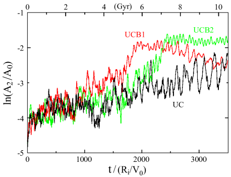
Figure 11: The time evolution of $A_{2}/A_{0}$ in simulations UC (black), UCB1 (red), and UCB2 (green). The top axis shows time scaled to physical units using the adopted scaling.

Figure 12: The power spectrum of $m=2$ density variations in simulation UC. The solid curve indicates the radius of corotation for the given frequency, while the dashed curves show the radii of the Lindblad resonances.

Since there are numerous disturbances with well scattered Lindblad resonances, random motion rises generally over the disc, as reported in Fig. 13, in contrast to Fig. 6 which shows the localized heating at the ILR of the single spiral case.

The larger changes in $L_{z}$ than those for the single spiral case are evident from the dot-dashed black curves of Fig. 14, which show the 5th and 95th percentiles of $\Delta L_{z}$ versus initial notional vertical amplitude $\zeta$. Although the shapes of these curves are similar to those in Fig. 7, they are asymmetric about zero indicating that gains are larger than losses.

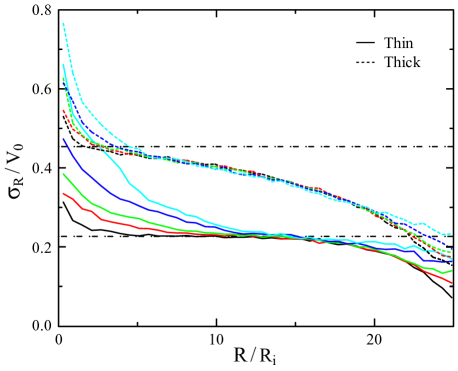
Figure 13: Radial variations of $\sigma_{R}$ in simulation UC for the thin (solid) and thick (dashed) discs. The curves are drawn at equal time intervals and $\sigma_{R}$ rises monotonically in the inner and outer discs.

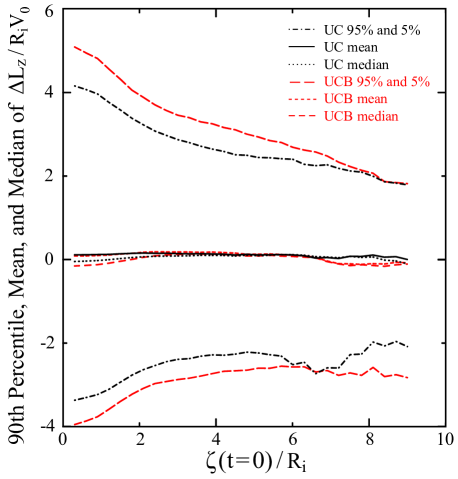
Figure 14: Same as Fig. 7 for simulations UC (dot-dashed black) and UCB1 (long-dashed red). The solid black and short-dashed red curves show the average angular momentum changes for UC and UCB1 respectively, and the dotted black and medium-dashed red ones show the median changes.

The angular momentum changes illustrated in Fig. 15 reflect mostly the effects of the latest spirals that developed in the simulation in each $L_{z}(t=0)$ region. Contours of changes to the distribution of home radii for the particles (dotted black and solid green in Fig. 16) reveal that particles from all initial radii can move to new home radii, but that the changes are greatest around the mid range of initial radii where corotation resonances are more likely. Some $0.003\%$ of the particles in the thin disc and $0.03\%$ in the thick end up on retrograde orbits.

Taken together with the results from the single spiral simulations described above, we again find that the changes in angular momenta and home radii are almost as great in the thick disc as in the thin. That is, radial migration is weakened only slightly by disc thickness.

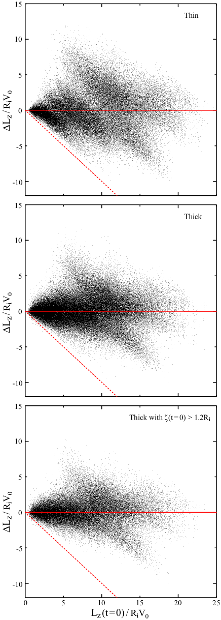
Figure 15: Same as Fig. 5 for simulation UC.

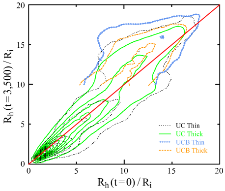
Figure 16: The distributions of final home radii versus initial home radii for all the particles in simulation UC. The particle density in this plane is estimated using an adaptive kernel, the dotted black and solid green contours represent the thin and thick discs respectively, and the red line shows zero change in $R_{h}$. Contour levels are chosen every $10\%$ of the thick disc’s maximum value from $5\%$ to $95\%$ for both thin and thick discs. The arrow light blue and dashed orange contours represent the same for the thin and thick discs of UCB1 respectively. The region inside the bar ($R_{h}(t=3500)<10R_{i}$) is omitted.

The top row of Fig. 17 shows changes in the UC particles’ maximum vertical excursions versus changes in their angular momenta. We find that, on average, $z_{\rm max}$ increases except for the greatest losses in angular momentum. This is different from the single spiral case, in which the contours and the mean and median curves are centred on the origin (Fig. 9). This overall extra increase in vertical amplitude probably comes from the net heating by vertical resonances that the multiple transient spirals induce by the end of the simulation. Nevertheless, the trend of the mean and median with $\Delta L_{z}$ remains as in M2. An exception is again the group of points along the slope of $-1$ in the second quadrant. It is much more pronounced for the thin disc than in M2. The particles contributing to this feature are still initially from the inner region of the disc, but this region is more extended in UC since the inner vertical resonances occur at various radii for the numerous transient spirals. As in M2, changes in $z_{\rm max}$ remain about twice as great for the thick disc particles as for those of the thin for the same $\Delta L_{z}$.

Although the scale height of outward migrating particles does increase somewhat, as expected, the changes are not substantial enough to cause the thickness of outward migrating thin-disc particles to approach the scale height of the thick disk. The changes in the vertical motion of inward migrating particles are more minor than those for outward migrators. Thus we do not observe much of a tendency in our models for evolution to cause a significant degree of blurring between the separate populations.

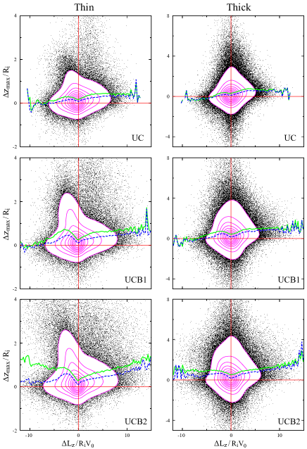
Figure 17: Same as Fig. 9 for simulations UC (top row), UCB1 (middle row), and UCB2 (bottom row). The left column shows $\Delta z_{\rm max}$ as a function of $\Delta L_{z}$ for the thin discs and the right for the thick.

5.2 Multiple spirals with a bar

We here study radial migration in two simulations, UCB1 and UCB2, that formed bars at an early stage of their evolution and compare them with simulation UC that did not form a bar for a long period. As noted in the introduction, it has long been known that bar formation causes some of the largest changes to the distribution of angular momentum within a disc. Here our focus is on the consequences of continued transient spiral behaviour in the outer disc long after the bar formed, which has not previously received much attention, as far as we are aware.

The red curve of Fig. 11 shows the evolution of $A_{2}/A_{0}$ in UCB1. The spirals become significant around the time $\sim 1\,000R_{i}/V_{0}$, the bar forms around $\sim 2\,000R_{i}/V_{0}$, and we stop the simulation at the same final time $t=3\,500R_{i}/V_{0}$ as UC. Thus, the time interval of significant scattering is roughly $2\,500R_{i}/V_{0}$ in length with a bar being present for the last $\sim 1\,500R_{i}/V_{0}$, which correspond to $7.5\;$Gyr and $4.5\;$Gyr respectively. With our suggested scaling, the bar has a pattern speed of $31.8\;$km s^-1 kpc^-1 and corotation $R_{c}\sim 7.5\;$kpc. (This scaling makes the bar substantially larger than that in the Milky Way.)

The long-dashed red curves in Fig. 14 show that the bar enhances the changes in $L_{z}$ somewhat over those that arise due to spirals alone. Note that we measure the instantaneous value of $L_{z}$ of each particle and it should be borne in mind that it changes continuously in the strongly non-axisymmetric potential of this model, especially so for particles in or near the bar.

For this reason, we cannot extend the light blue (marked with arrow heads) and dashed orange contours in Fig. 16 to small home radii at the later time in the strongly non-axisymmetric potential of the bar. However, a clear asymmetry can be seen; the distribution is biased above the zero change red line, indicating a systematic outward migration in the outer disc. A similar asymmetry can be seen without a bar in UC (dotted black and solid green contours), but the formation of the bar makes it more pronounced. Since total angular momentum is conserved in these simulations, there is a corresponding inward migration in the inner regions (see Fig. 5).

Aside from the bar region, where systematic non-circular streaming biases the rms radial velocities, Fig. 18 shows that the bar does not appear to cause much extra heating over that in the unbarred case.

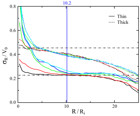
Figure 18: Same as Fig. 13 for UCB1.

Fig. 19 again illustrates that changes in $L_{z}$ in the outer disc are more substantial in this barred model than in the unbarred case (Fig. 15), but the larger spread in $\Delta L_{z}$ in the inner disc is partly an artifact of using the instantaneous values of $L_{z}$ at later times. Because we use the instantaneous $L_{z}$ in the barred potential in this Figure, a particle in the region where $\Delta L_{z}<-L_{z}$ need not necessarily have been changed to a fully retrograde orbit.

The asymmetries in Figs. 16 & 19 about the red lines of zero change are not caused by bar-formation alone, as the distributions (not shown) are approximately symmetric immediately after this event. Rather, we find they appear to be caused by multiple migrations of the same particles by separate events.

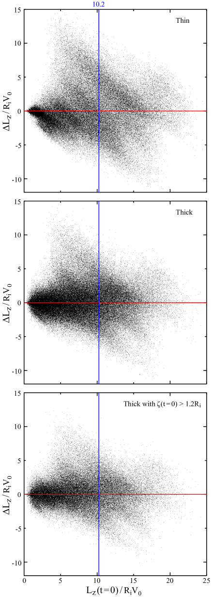
Figure 19: Same as Fig. 15 for simulation UCB1. The vertical blue line marks the approximate corotation resonance of the bar.

Our second barred simulation, UCB2, again differs from UCB1 and UC only by the initial random seed. It formed a stronger bar, but a little later than in UCB1, as shown by the green curve of Fig. 11. Significant scattering occurs for the last $\sim 1\,800R_{i}/V_{0}$ time units ($5.4\;$Gyr) of which the bar is present for the last $\sim 1\,100R_{i}/V_{0}$ ($3.3\;$Gyr). The pattern speed ($33.6\;$km s^-1 kpc^-1) and corotation radius ($\sim 7.3\;$kpc) for our adopted scaling, are similar to the values in UCB1.

We find the extent of radial migration (bottom two rows of Table 3) is further increased by the stronger bar, but not by much. Variants of Figs. 19 & 16 (not shown) are qualitatively similar with slightly larger changes, but the outer disc is again dominated by scattering due to the latest few spirals.

In both these models, therefore, we see that the formation of a bar does indeed increase the net angular momentum changes. However the overall behaviour is similar to that of scattering by transient spirals without a bar. This is different from the effect found by Brunetti et al. (2011), in which essentially all the angular momentum changes occurred during bar formation.

The lower two rows of Fig. 17 show $\Delta z_{\rm max}$ versus $\Delta L_{z}$ for UCB1 and UCB2 respectively. The presence of a bar yields a much denser and more extended feature in the second quadrant, which is also visible in for thick disc. For UCB2, its contribution is so great that the mean $\Delta z_{\rm max}$ keeps increasing with greater angular momentum loss. This extra apparent vertical heating is probably caused by the buckling of the bar. Unlike for M2, UC, and UCB1, we find that for positive $\Delta L_{z}$ in UCB2, the mean and median curves keep rising for larger $\Delta L_{z}$.

6 A Conserved Quantity?

Radial migration results from angular momentum changes near corotation, which we have shown to be somewhat weakened by increased vertical motion. Schönrich & Binney (2009a), in their model of radial mixing in thin and thick discs, assumed that vertical and radial motions are decoupled and that vertical energy is conserved as stars migrate radially. We here try to identify a conserved quantity that can be used to predict vertical motion when particles suffer large changes in $L_{z}$, by comparing various measures of vertical amplitude at the initial and final times in simulations with a single spiral. Note that the “initial” value of each quantity we discuss in this section is measured at $t=64R_{i}/V_{0}$, which avoids possible effects of the settling of the model from its mild initial imbalance. Also, all quantities are computed in an azimuthally averaged potential, to eliminate variations with spiral phase, which remain significant at the final time.

We focus on particles whose initial home radii lie in an annulus of width $6.0R_{i}$ centred at corotation of the spiral in M2, and measure quantities for only one particle per quiet start ring, meaning one in every twelve. This results in $\sim 40\,000$ particles from the thin disc and $\sim 73\,000$ from the thick. Although the entire thick disc is represented by just 50% more particles than is the thin, the effects of the inner and outer tapers, together with the groove in the thin disc cause the number of particles in the range $4.0R_{i}\leq R_{h}(t=64)\leq 10.0R_{i}$ to be some 82% larger for the thick disc than for the thin. While we endeavour to measure each quantity in this section for the same set of particles, from both simulations M2 and T, we have been able to estimate some quantities for only a subset of these particles, as noted below.

Figure 20: The top left panel shows a typical thick disc orbit in the meridional plane, and the other three panels show how $E_{z,R}$ varies with time (top right), radius (bottom left), and $z$-height (bottom right). The particle, which has a home radius of $6.5R_{i}$, a total energy of $-2.0V_{0}^{2}$, a midplane eccentricity of $0.15$, and a vertical excursion of $2.1R_{i}$, is integrated in the frozen initial axisymmetric potential of simulation M2.

6.1 Vertical energies

We have tried a number of different way to estimate the energy of vertical motion. A simple definition might be

$$E_{z,R}=\frac{1}{2}v_{z}^{2}+\Phi(R,z)-\Phi(R,0),$$ (13)

with $R$ being the instantaneous radius of the particle. However, Fig. 20 shows that $E_{z,R}$ defined this way varies by some 30% as a particle oscillates in both radius and vertically in a static axisymmetric potential. The orbit of this particle is multiply periodic and clearly respects three integrals (as we will confirm below), in common with many orbits in axisymmetric potentials (BT08, section 3.2). Although such orbits can be described by action-angle variables, which imply three decoupled oscillations, the energy of vertical motion is clearly not decoupled from that of the radial part of the motion. In particular, the bottom left panel shows that $E_{z,R}$ varies systematically with radius, which reflects in part the weakening of the vertical restoring force with the outwardly declining surface density of the disc. This behaviour considerably complicates our attempts to compare the vertical energies at two different times in the same simulation.

The epicycle approximation (BT08, p. 164) holds for stars whose orbits depart only slightly from circular motion in the midplane. In this approximation, when a star pursues a near-circular orbit near the mid-plane of an axisymmetric potential, the vertical and radial parts of the motion are separate, decoupled oscillations, and the vertical energy is $E_{z,\rm epi}\;(=Z$ eq. 8) is constant. However, the epicycle approximation is a poor description of the motion of most particles, for which the radial and vertical oscillations are neither harmonic nor are the energies of the two oscillations decoupled.

Table 4 gives the rms values of $[Y(t_{\rm final})-Y(t_{\rm initial})]/Y(t_{\rm initial})$ for particles in both the thin and the thick discs of simulations M2 and T. Here $Y$ represents one of several possible vertical integrals. The first rows give the fractional changes in the epicycyclic approximation, $Y=E_{z,\rm epi}$, that are substantial. Furthermore, they are almost as large in simulation T, which was constrained to remain axisymmetric, as those in M2 in which substantial radial migration occurred, suggesting that the changes are mostly caused by the inadequacy of the approximation.

Table 4: Biweight standard deviation of fractional changes in various estimates of vertical energy and action.

Simulation	Disc	Variable $Y$	$\sigma(\Delta Y/Y_{\rm initial})$
M2	Thin	$E_{z,\rm epi}$	30.7%	28.9%
		$E_{z,R}$	28.3%	27.2%
		$E_{z,R_{h}}$	25.0%	26.1%
		$\langle E_{z,R}\rangle$		23.6%
		$J_{z,\rm epi}$	22.7%	20.7%
		$J_{z}|_{R,\phi}$	16.5%	16.0%
		$J_{z}$		15.6%
	Thick	$E_{z,\rm epi}$	59.4%	39.4%
		$E_{z,R}$	47.6%	31.5%
		$E_{z,R_{h}}$	34.9%	26.0%
		$\langle E_{z,R}\rangle$		22.3%
		$J_{z,\rm epi}$	55.7%	34.9%
		$J_{z}|_{R,\phi}$	35.0%	19.7%
		$J_{z}$		15.4%
T	Thin	$E_{z,\rm epi}$	22.5%	19.5%
		$E_{z,R}$	17.9%	15.4%
		$E_{z,R_{h}}$	10.0%	8.8%
		$\langle E_{z,R}\rangle$		5.8%
		$J_{z,\rm epi}$	16.5%	13.8%
		$J_{z}|_{R,\phi}$	9.4%	8.2%
		$J_{z}$		6.1%
	Thick	$E_{z,\rm epi}$	53.6%	34.3%
		$E_{z,R}$	40.8%	22.8%
		$E_{z,R_{h}}$	23.3%	11.4%
		$\langle E_{z,R}\rangle$		3.0%
		$J_{z,\rm epi}$	47.5%	27.8%
		$J_{z}|_{R,\phi}$	24.8%	11.0%
		$J_{z}$		3.4%

The biweight estimated standard deviation of the fractional change in variable $Y$ listed in the third column for both the thin and thick discs in simulations M2 and T. We give two values for the standard deviation in some rows: the value in the fourth column is measured from all the particles, that in the fifth column is from only the 48% (in M2) of particles for which $\Delta J_{z}$ is calculable.

The second rows in Table 4 show the rms fractional changes in the instantaneous values of $E_{z,R}$. While these values are slightly smaller than for the epicyclic estimate, they are again large for the thin disc and still greater for the thick. This is hardly surprising, as the particles in the simulation have random orbit phases at the two measured times.

Particles on eccentric orbits generally spend more time at radii $R>R_{h}$ than inside this radius, which biases the instantaneous measure to a lower value, as shown in the third panel of Fig. 20. To eliminate this bias, and to reduce the random variations, we evaluate $E_{z,R_{h}}$ from eq. (13) at the home radius of each particle, which requires us to integrate the motion of each particle in the frozen potential of the appropriate time until the particle reaches its home radius. A tiny fraction, $\sim 500$ of the $\sim 113\,000$ sample particles, never cross $R=R_{h}$ at the initial time and $\sim 200$ more at the final time; these particles rise to large heights above the mid-plane and have meridional orbits resembling that shown in the top right of Fig. 25, but appear to be confined to $R>R_{h}$. The fact that this is possible seems consistent with the description of vertical oscillations developed by Schönrich & Binney (2012). The third rows of Table 4 give the fractional rms changes in $E_{z,R_{h}}$ for all the remaining particles; the changes in simulation M2 are a little smaller than those of the instantaneous values and significantly so in simulation T.

Since $E_{z,R}$ is multiply periodic (Fig. 20), we have also estimated an orbit-averaged value, $\langle E_{z,R}\rangle$, by integrating the motion for many periods until the time average changed by $<0.1\%$ when the integration is extended for an additional radial period. The fourth rows of Table 4 give the rms changes in $\langle E_{z,R}\rangle$, which are still considerable. Note that we did not compute this time-consuming estimate for all the particles, but for only the subset used for other values in the fifth column of this table. The choice of this subset is described below.

Generally, we find that none of these estimates of the vertical energy is even approximately conserved, except for the orbit-averaged energy when the simulation is constrained to remain axisymmetric (simulation T). In this case, the potential at the two times differs slightly due to radial variations in the mass distribution – values of this orbit-averaged quantity in an unchanged potential would be independent of the moment at which the integration begins.

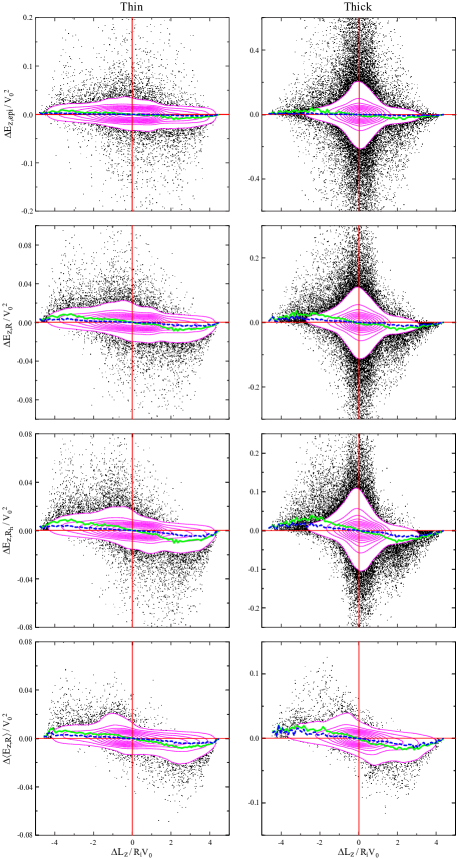
Figure 21: Changes in $E_{z,\rm epi}$ (first row), $E_{z,R}$ (second row), $E_{z,R_{h}}$ (third row), and $\langle E_{z,R}\rangle$ (fourth row) versus $\Delta L_{z}$ for the thin (left column) and thick (right column) discs of simulation M2. Just as in Fig. 9, the horizontal and vertical red lines show zero changes, the linearly spaced magenta contours show number density, and the bold solid green and dashed blue curves show the mean and median changes in each ordinate respectively. Note that the vertical scales differ in each plot.

In all cases, changes are larger in simulation M2 where significant radial migration occurs. Fig. 21 illustrates that the changes in the estimated vertical energy correlate with $\Delta L_{z}$. The excesses of particles in the second and fourth quadrants indicate that changes have a tendency to be negative for outwards migrating particles and positive for inwards migrating particles. The significance of this trend is discussed below.

6.2 Vertical actions

The various actions of a regular orbit in a steady potential are defined to be $(2\pi)^{-1}$ times the appropriate cross-sectional area of the orbit torus (BT08, pp. 211–215). One advantage of actions is that they are the conserved quantities of an orbit when the potential changes slowly – i.e. they are adiabatic invariants under conditions that are defined more carefully in BT08 (pp. 237–238).

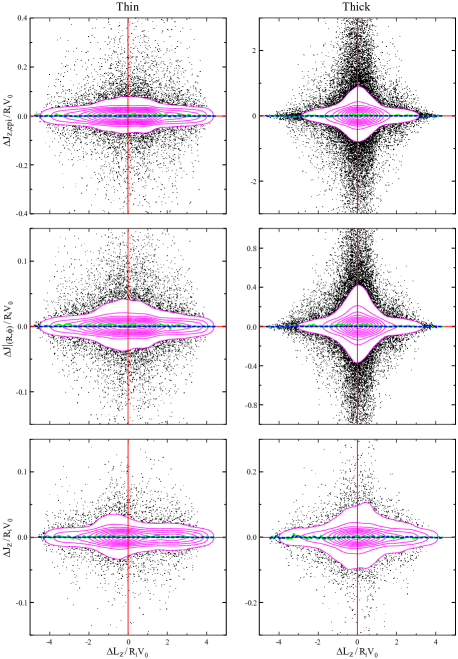
Figure 22: Same as Fig. 21 for changes in $J_{z,\rm epi}$ (first row), $J_{z}|_{R,\phi}$ (second row), and $J_{z}$ (third row) of the particles in M2.

The vertical action is defined as

$$J_{z}\equiv{1\over 2\pi}\oint\dot{z}dz,$$ (14)

where $z$ and $\dot{z}$ are measured in some suitable plane that intersects the orbit torus. Since $L_{z}\;(\equiv J_{\phi})$ is conserved in a steady axisymmetric potential, the orbit can be followed in the meridional plane (BT08, p159) in which it oscillates both radially and vertically, as illustrated in the first panel of Fig. 20. To estimate $J_{z}$, we need to integrate the orbit of a particle in a simulation from its current position in the frozen, azimuthally averaged potential at that instant and construct the $(z,\dot{z})$ surface of section (SoS) as the particle crosses $R_{h}$ with $\dot{R}>0$, say. The integral in eq. (14) is the area enclosed by an invariant curve in this plane.

Before embarking on this elaborate procedure, we consider two possible approximations. When the epicycle approximation holds, the vertical action is $J_{z,\rm epi}=E_{z,\rm epi}/\nu$ (BT08 p. 232). The fifth rows of Table 4 for each disc show that changes in this quantity are large and again they are similar to those in simulation T, confirming once again that the epicycle approximation is inadequate.

Since most orbits reach beyond the harmonic region ($|z|\la 0.4R_{i}$) of the vertical potential, an improved local approximation is to calculate

$$J_{z}|_{R,\phi}=\left.(2\pi)^{-1}\oint\dot{z}dz\right|_{R,\phi}$$ (15)

at the particle’s fixed position in the disc. This local estimate still ignores the particle’s radial motion, but gives a useful estimate for the average vertical action that is also used in analytic disc modeling (Binney, 2010). The function $\dot{z}(z)$ at this fixed point is simply determined by the vertical variation of $\Phi(R,\phi,z)$, and the area is easily found. We evaluate $J_{z}|_{R,\phi}$ at the particle’s instantaneous position at the initial and final times using the corresponding azimuthally averaged frozen potential. The rms variation of $\Delta J_{z}|_{R,\phi}$ is given in the sixth rows of Table 4 for each disc. We find that $\Delta J_{z}|_{R,\phi}$ in the thin discs of both M2 and T are small, suggesting that this estimate of vertical action is more nearly conserved. However, the changes for the thick discs are still large, and we conclude that this local estimate is still too approximate.

We therefore turn to an exact evaluation of eq. (14) using the procedure described in the Appendix. Unfortunately, we can evaluate $\Delta J_{z}$ only if the consequents in the SoS form a simple invariant curve that allows $J_{z}$ to be estimated at both times. We find that only 48% of the $\sim 113\,000$ particles have closed, concave invariant curves at the initial time and only 73% of those retain these properties at the final time. Although the thick disc contains more particles than the thin, we are able to calculate $\Delta J_{z}$ for a smaller fraction: we succeed with $\sim 26\,000$ in the thin disc but only $\sim 13\,000$ in the thick.

Column five of Table 4 gives the rms changes of all estimates of vertical energy and action for only these particles. While the fractional rms values of the different energy estimates remain large, they are generally smaller than those for the all particles given in the fourth column, but only slightly so for $J_{z}|_{R,\phi}$. Thus the orbits for which $\Delta J_{z}$ can be computed are not a random subset, but are biased to those for which energy changes are smaller on average.

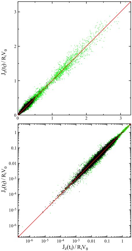
Figure 23: Comparison of $J_{z}$ for $\sim 40\,000$ particles from simulation M2 at the initial and final times. Values are calculated from eq. (14). The top panel is on a linear scale, the bottom on a log scale to reveal the behaviour for very small actions. The red line has unit slope. Thin disc particles are marked in black, thick disc in green.

The seventh (final) rows of Table 4 for each disc list the rms values of the fractional change in $\Delta J_{z}$. They are just a few percent for particles in simulation T, in which the disc is constrained to remain axisymmetric, and are smaller than for any other tabulated quantity in the discs perturbed by a spiral. The small scatter about the red line of unit slope in Fig. 23 indicates that differences in the final and initial values of $J_{z}$ in both discs for M2 are indeed small.

Fig. 22 shows that changes in all three estimators of the vertical actions are uncorrelated with $\Delta L_{z}$, and that the mean and median changes are close to zero. Comparison with the systematic changes in Fig. 21 suggest that $J_{z}$ is, in fact, conserved. To see this, note that changes in $L_{z}$ shift the home radius of each particle to a region where the average vertical restoring force differs, the amplitudes of the vertical oscillations increase due to the weaker average restoring force when $\Delta L_{z}>0$, and conversely decrease for $\Delta L_{z}>0$. Thus if an estimator of vertical motion is not conserved, we should expect a systematic variation with $\Delta L_{z}$, as we observe for all the energy estimators in Fig. 21. The fact that there is no systematic variation of the median or mean change in vertical action suggest that it is conserved.

If $J_{z}$ is a conserved quantity, it may seem puzzling that the rms changes in our measurements are not smaller. Both $J_{z,\rm epi}$ and $J_{z}|_{R,\phi}$ are approximate, which could be responsible for apparent substantial changes, but changes in the “exact” estimate of $J_{z}$ remain significant, even for simulation T. It is possible that our estimate of $\Delta J_{z}$ is inaccurate. For example, we must eliminate non-axisymmetric structure from the potential to compute $J_{z}$, introducing small errors when the potential is mildly non-axisymmetric. Larger differences could arise, however, if the invariant curve changes its character, especially since entering or leaving a trapped area in phase space is not an adiabatic change. It is possible an orbit that appears to be unaffected by resonant islands in phase space at the initial and final times could have experienced trapping about resonant islands for some of the intermediate evolution, allowing $J_{z}$ to change even when changes to the potential are indeed slow.

We have verified that $J_{z}$ is conserved to a part in $10^{4}$ in a further simulation with a frozen, axisymmetric potential. Note this is not a totally trivial test, since we use the $N$-body integrator and the grid-determined accelerations to advance the motion for $\sim 350$ dynamical times before making our second estimate. Therefore the non-zero changes in simulation T are indeed caused by changes to the potential. Even though the potential variations are small, substantial action changes indicate that changes to the orbit were non-adiabatic, which can happen for the reason given in the previous paragraph. Our “initial” $J_{z}$ values are estimated at $t=64R_{i}/V_{0}$, when we believe the model has relaxed from the initial set up; we therefore suspect that the small potential variations are more probably driven by particle noise, which can be enhanced by collective modes (Weinberg, 1998). This hypothesis is supported by our finding variations in $J_{z}$ that were about ten times greater than in simulation T when we employed 100 times fewer particles.

7 Summary

We have presented a quantitative study of the extent of radial migration in both thin and thick discs in response to a single spiral wave. We find angular momentum changes in the thick disc are generally smaller than those in the thin, although the tail to the largest changes in each population is almost equally extensive.

We have introduced populations of test particles into a number of our simulations in order to determine how changes in $L_{z}$ vary with disc thickness and with radial velocity dispersion when subject to the same spiral wave, finding an exponential decrease in $\left\langle(\Delta L_{z})^{2}\right\rangle^{1/2}$, as shown in Fig. 10.

We find that spirals of smaller spatial scale cause smaller changes. When we were careful to change all the properties of the model by the appropriate factors, we were able to account for smaller changes to $\left\langle(\Delta L_{z})^{2}\right\rangle^{1/2}$ as being due to a combination of the weakened spiral amplitude near corotation and the change in the value of $m$. Furthermore, we found evidence that the saturation amplitude scales inversely as $m$, in line with the theory developed by Sellwood & Binney (2002). Note the simple scaling holds true only when the principal dynamical properties, such as $Q$, $X$, thickness, and gravity softening, are held fixed relative to the scale of the mode. Nevertheless, it seems reasonable to expect smaller changes to $\left\langle(\Delta L_{z})^{2}\right\rangle^{1/2}$ in general for spirals higher $m$. The exponential decrease of $\left\langle(\Delta L_{z})^{2}\right\rangle^{1/2}$ with increasing disc thickness applies only for different populations subject to the same spiral perturbation.

We have also run slightly more realistic simulations to follow the extent of churning in both thick and thin discs that are subject to large numbers of transient spiral waves having a variety of rotational symmetries. Fig. 16 shows that changes in the home radii of thick disc particles are smaller on average than those of the thin disc, but again the tails of the distributions in both populations are almost co-extensive. As found in previous work (Friedli, Benz & Kennicutt, 1994; Raboud et al., 1998; Grenon, 1999; Debattista et al., 2006; Minchev et al., 2011; Bird, Kazantzidis & Weinberg, 2011), the formation of a bar also causes substantial angular momentum changes within a disc, but we find that the churning effect from multiple spiral patterns still dominates changes in the outer disc after the bar has formed.

We find that vertical action is conserved during radial migration, despite the fact that relative changes in our estimated $J_{z}$, which can be measured for only about half the particles, are as large as $\sim 15\%$. Because the vertical restoring force to the mid-plane decreases outwards, an increased (decreased) home radius causes the particle to experience a systematically weaker (stronger) vertical restoring force, making it impossible for both vertical energy and action to be conserved. We find a clear systematic variation of the vertical energy with $\Delta L_{z}$, but none with $\Delta J_{z}$ leading us to conclude that vertical action is the conserved quantity. The residual scatter in our measured values of $\Delta J_{z}$ could be caused by trapping and escape from multiply-periodic resonant islands in phase space, as well as numerical jitter in the $N$-body potential, as we discuss at the end of §6. In the absence of these complications, we believe that the vertical action is conserved.

Thus conservation of vertical action, and not of vertical energy, should be used to prescribe the changes to vertical motion in models of chemo-dynamic evolution. It would be especially useful to obtain diffusion coefficients that include the effects of radial migration as functions of radius and height due to a transient spiral or a combination of consecutive spirals with various corotation radii. We leave this work to a future paper.

Appendix A Numerical estimate of vertical action

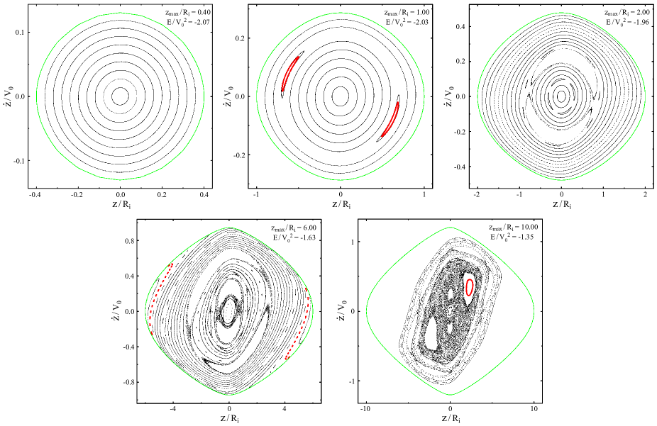
Figure 24: Surfaces of section in the $(z,\dot{z})$ plane, when $R=R_{h}$ and $\dot{R}>0V_{0}$, for test particles in the initial potential of simulation M2. All particles in each panel have the same total energy and corresponding $z_{rmmax}$, which are noted in the top right corner. The outer most green curves mark the zero-velocity curves, at which $\dot{R}=0V_{0}$ for the given $z$, $L_{z}$ and $E$. Finally, the bold red curves are from the three orbits shown in Fig. 25.

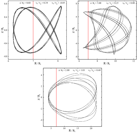
Figure 25: Orbits in the meridional plane of the three test particles drawn in bold red in the second, fourth and fifth panels of Fig. 24. Note that we show only a small fraction of the full orbit used to produce the invariant curves in the $(z,\dot{z})$ plane. The vertical red lines mark $R_{h}$ at which the SoS is constructed. The initial vertical position and radial and vertical velocities of each of these three particles are noted.

Fig. 24 illustrates the SoS for five different energies, all for $L_{z}=7$. Each invariant curve is generated by a test particle in the initial potential of M2. All the particles in one panel have the same energy and angular momentum (noted in the top right corner), but differ in the extent of their vertical motion. The zero-velocity curve, where a particle’s radial velocity must be zero for the $L_{z}$ and $E$ values adopted is the outer most green curve. We see that most of phase space is regular, but not all consequents mark out simple closed invariant curves; some significant fraction of phase space is affected by islands in the SoS that surround multiply periodic orbits. Chaotic motion, in which consequents fill an area rather than lie on a closed curve in the SoS, is extensive only for the greatest energy.

The paths in the meridional plane of three multiply periodic orbits are shown in Fig. 25. They correspond to the bold red invariant curves in the second, fourth, and fifth SoS panels of Fig. 24. The last orbit has almost equal radial and vertical periods and circulates only clockwise in the meridional plane. Since we plot only when the particle passes $R_{h}$ with $\dot{R}>0V_{0}$, the consequents lie only in the first quadrant of the $(z,\dot{z})$ plane. Were we to plot the other crossing instead, where $\dot{R}<0V_{0}$, the invariant curve would be a reflected image in the second quadrant. Also, had we chosen the negative root for initial radial velocity, the particle would have circulated only counterclockwise and yielded a $180^{\circ}$-rotationally symmetric invariant curve in the third quadrant. This accounts for the skewness of the invariant curves in the SoS, which diminishes for particles of lower energy.

The area in the SoS enclosed by only those orbits having a simple invariant curve yields a numerical estimate of the vertical action $J_{z}$. We find all the consequents for a particle as its motion advances over $7\times 10^{4}$ dynamical times from its position in the frozen, azimuthally averaged, potential, and make a numerical estimate of the area integral (eq. 14).

We repeat this exercise at both the initial and final times in the simulation.

References

- (1)
- Abadi et al. (2003) Abadi, M. G., Navarro, J. F., Steinmetz, M. & Eke, V. R. 2003, ApJ, 597, 21
- Beers et al. (1990) Beers, T. C., Flynn, K. & Gebhardt, K. 1990, AJ, 100, 32
- Bensby et al. (2005) Bensby, T., Feltzing, S., Lundström, I. & Ilyin, I. 2005, A&A, 433, 185
- Binney (2010) Binney, J. 2010, MNRAS, 401, 2318
- Binney & Lacey (1988) Binney, J. J. & Lacey, C. G. 1988, MNRAS, 230, 597
- Binney & Tremaine (2008) Binney, J. & Tremaine, S. 2008, Galactic Dynamics. Princeton Univ. Press, Princeton (BT08)
- Bird, Kazantzidis & Weinberg (2011) Bird, J. C., Kazantzidis, S. & Weinberg, D. H. 2011, MNRAS, submitted (arXiv:1104.0933)
- Bournaud & Combes (2002) Bournaud, F. & Combes, F. 2002, A&A, 392, 83
- Bournaud, Elmegreen & Martig (2009) Bournaud, F., Elmegreen, B. G. & Martig, M. 2009, ApJ, 707, L1
- Bovy et al. (2011) Bovy, J., Rix, H-W., Liu, C., Hogg, D. W., Beers, T. C. & Lee, Y. S. 2011, arXiv:1111.1724
- Brook et al. (2005) Brook, C. B., Gibson, B. K., Martel, H. & Kawata, D. 2005, ApJ, 630, 298
- Brunetti et al. (2011) Brunetti, M., Chiappini, C. & Pfenniger, D. 2011, A&A, 534, A75
- Camm (1950) Camm, G. L. 1950, MNRAS, 110, 305
- Chiba & Beers (2000) Chiba, M. & Beers, T. C. 2000, AJ, 119, 2843
- Debattista et al. (2006) Debattista, V. P., Mayer, L., Carollo, C. M., Moore, B., Wadsley, J. & Quinn, T. 2006, ApJ, 645, 209
- D’Onghia et al. (2010) D’Onghia, E., Springel, V., Hernquist, L. & Keres, D. 2010, ApJ, 709, 1138
- Evans & Read (1998) Evans, N. W. & Read, J. C. A. 1998, MNRAS, 300, 106
- Friedli, Benz & Kennicutt (1994) Friedli, D., Benz, W. & Kennicutt, R. 1994, ApJL, 430, L105
- Fuhrmann (2008) Fuhrmann, K. 2008, MNRAS384, 173
- Gilmore & Reid (1983) Gilmore, G. & Reid, N. 1983, MNRAS, 202, 1025
- Grenon (1999) Grenon, M. 1999, Ap. Sp. Sci., 265, 331
- Hänninen & Flynn (2002) Hänninen, J. & Flynn, C. 2002, MNRAS, 337, 731
- Helmi et al. (2006) Helmi, A., Navarro, J. F., Nordström, B., Holmberg, J., Abadi, M. G. & Steinmetz, M. 2006, MNRAS, 365, 1309
- Hohl (1971) Hohl, F. 1971, ApJ, 168, 343
- Ivezić et al. (2008) Ivezić, Ž. et al.2008, AJ, 684, 287
- Jurić et al. (2008) Jurić, M. et al.2008, AJ, 673, 864
- Kazantzidis et al. (2008) Kazantzidis, S., Bullock, J. S., Zentner, A. R., Kravtsov, A. V. & Moustakas, L. A. 2008, ApJ, 688, 254
- Kregel, van der Kruit & de Grijs (2002) Kregel, M., van der Kruit, P. C. & de Grijs, R. 2002, MNRAS, 334, 646
- Lee et al. (2011) Lee, Y. S. et al. 2011, ApJ, 738, 187
- Loebman et al. (2011) Loebman, S. R., Ros̆kar, R., Debattista, V. P., Ivezić, Z̆., Quinn, T. R. & Wadsley, J. 2011, ApJ, 737, 8
- Majewski (1993) Majewski, S. R. 1993, ARAA, 31, 575
- Martínez-Serrano et al. (2009) Martínez-Serrano, F. J., Serna, A., Doménech-Moral, M. & Domínguez-Tenreiro, R. 2009, ApJ, 705, L133
- Mestel (1963) Mestel, L. 1963, MNRAS, 126, 553
- Monaghan (1992) Monaghan, J. J. 1992, ARAA, 30, 543
- Minchev & Famaey (2010) Minchev, I. & Famaey, B. 2010, ApJ, 722, 112
- Minchev et al. (2011) Minchev, I., Famaey, B., Combes, F., Di Matteo, P., Mouhcine, M. & Wozniak, H. 2011, A&A, 527, A147
- Munn et al. (2004) Munn, J. A. et al. 2004, AJ, 127, 3034
- Quillen et al. (2009) Quillen, A. C., Minchev, I., Bland-Hawthorn, J. & Haywood, M. 2009, MNRAS, 397, 1599
- Quinn, Hernquist & Fullagar (1993) Quinn, P. J., Hernquist, L. & Fullagar, D. P. 1993, ApJ, 403, 74
- Raboud et al. (1998) Raboud, D., Grenon, M., Martinet, L., Fux, R. & Udry, S. 1998, A&A, 335, L61
- Reddy, Lambert & Allende Prieto (2006) Reddy, B. E., Lambert, D. L. & Allende Prieto, C. 2006, MNRAS, 367, 1329
- Ros̆kar et al. (2008a) Ros̆kar, R., Debattista, V. P., Quinn, T. R., Stinson, G. S. & Wadsley, J. 2008a, ApJL, 684, L79
- Ros̆kar et al. (2008b) Ros̆kar, R., Debattista, V. P., Stinson, G. S., Quinn, T. R., Kaufmann, T. & Wadsley, J. 2008b, ApJL, 675, L65
- Sánchez-Blázquez et al. (2009) Sánchez-Blázquez, P., Courty, S., Gibson, B. K. & Brook, C. B. 2009, MNRAS, 398, 591
- Scannapieco et al. (2011) Scannapieco, C., White, S. D. M, Springel, V. & Tissera, P. B. 2011, MNRAS, 417, 154
- Schönrich & Binney (2009a) Schönrich, R. & Binney, J. 2009, MNRAS, 396, 203
- Schönrich & Binney (2009b) Schönrich, R. & Binney, J. 2009, MNRAS, 399, 1145
- Schönrich & Binney (2012) Schönrich, R. & Binney, J. 2012, MNRAS, 419, 1546
- Sellwood (1985) Sellwood, J. A. 1985, MNRAS, 217, 127
- Sellwood (2010) Sellwood, J. A. 2010, in Planets Stars and Stellar Systems, v.5, ed. G. Gilmore (Heidelberg: Springer) to appear (arXiv:1006.4855)
- Sellwood (2012) Sellwood, J. A. 2012, ApJ, submitted
- Sellwood & Athanassoula (1986) Sellwood, J. A. & Athanassoula, E. 1986, MNRAS, 221, 195
- Sellwood & Binney (2002) Sellwood, J. A. & Binney, J. J. 2002, MNRAS, 336, 785
- Sellwood & Carlberg (1984) Sellwood, J. A. & Carlberg, R. G. 1984, ApJ, 282, 61
- Sellwood & Debattista (2009) Sellwood, J. A. & Debattista, V. P. 2009, MNRAS, 398, 1279
- Sellwood & Kahn (1991) Sellwood, J. A. & Kahn, F. D. 1991, MNRAS, 250, 278
- Sellwood & Preto (2002) Sellwood, J. A. & Preto, M. 2002, In ”Disks of Galaxies. Kinematics. Dynamics and Perturbations.”, Astron. Soc. Pac., Eds. E. Athanassoula & A. Bosma A. (San Francisco)
- Sellwood & Valluri (1997) Sellwood, J. A. & Valluri, M. 1997, MNRAS, 287, 124
- Shen & Sellwood (2004) Shen, J. & Sellwood, J. A. 2004, ApJ, 604, 614
- Spitzer (1942) Spitzer, L. 1942, ApJ, 95, 329
- Spitzer & Schwarzschild (1953) Spitzer, L. & Schwarzschild, M. 1953, ApJ, 118, 106
- Toomre (1977) Toomre, A. 1977, ARAA, 15, 437
- Toomre (1981) Toomre, A. 1981, In ”The Structure and Evolution of Normal Galaxies”, Eds. S. M. Fall & D. Lynden-Bell (Cambridge, Cambridge Univ. Press) p. 111
- Toomre (1982) Toomre, A. 1982, ApJ, 259, 535
- van der Kruit & Freeman (2011) van der Kruit, P. C. & Freeman, K. C 2011, ARAA, 49, 301
- Villalobos & Helmi (2008) Villalobos, Á. & Helmi A. 2008, MNRAS, 391, 1806
- Weinberg (1998) Weinberg, M. D. 1998, MNRAS, 297, 101
- Wyse (2009) Wyse, R. F. G. 2009, In “The Galaxy Disk in Cosmological Context”, IAU Symposium 254. Eds. J. Andersen, J. Bland-Hawthorn & B. Nordström (Cambridge, Cambridge University Press) p. 179 (arXiv:0809.4516)
- Yoachim & Dalcanton (2006) Yoachim, P. & Dalcanton, J. J. 2006, AJ, 131, 226
- York et al. (2000) York, D. G., et al. 2000, AJ, 120, 1579
- Yu et al. (2012) Yu, J-C., Sellwood, J. A., Pryor, C. Hou, J-L. & Li, C. 2012, ApJ, (submitted)
- Zang (1976) Zang, T. A. 1976, PhD. thesis, MIT