Oscillating universe in the DGP braneworld

Abstract

With a method in which the Friedmann equation is written in a form such that evolution of the scale factor can be treated as that of a particle in a “potential”, we classify all possible cosmic evolutions in the DGP braneworld scenario with the dark radiation term retained. By assuming that the energy component is pressureless matter, radiation or vacuum energy, respectively, we find that in the matter or vacuum energy dominated case, the scale factor has a minimum value $a_{0}$. In the matter dominated case, the big bang singularity can be avoided in some special circumstances, and there may exist an oscillating universe or a bouncing one. If the cosmic scale factor is in the oscillating region initially, the universe may undergo an oscillation. After a number of oscillations, it may evolve to the bounce point through quantum tunneling and then expand. However, if the universe contracts initially from an infinite scale, it can turn around and then expand forever. In the vacuum energy dominated case, there exists a stable Einstein static state to avoid the big bang singularity. However, in certain circumstances in the matter or vacuum energy dominated case, a new kind of singularity may occur at $a_{0}$ as a result of the discontinuity of the scale factor. In the radiation dominated case, the universe may originate from the big bang singularity, but a bouncing universe which avoids this singularity is also possible.

I Introduction

The modified gravity has spurred an increasing deal of interest recently, because it can explain, without the introduction of an exotic dark energy, the present accelerating cosmic expansion discovered firstly from the Type Ia Supernovae (Sne Ia) Perlmutter1999 ; Riess1998 ; Riess2004 ; Riess2006 ; Astier2006 ; Wood2007 . Among the modified gravity theories, the Dvali-Gabadadze-Porrati (DGP) braneworld scenario Dvali2000 , generalized firstly to cosmology by Deffayet Deffayet2001 , is a very simple and popular one. The DGP theory starts with the idea that our observed four-dimensional Universe resides in a five-dimensional, infinite-volume Minkowski bulk and the whole energy-momentum is confined on a three dimensional spacial brane. In contrast to the Randall-Sundrum Randall1999 and Shtanov-Sahni Shtanov2003 braneworld scenarios with high energy modifications to general relativity, the DGP brane produces a low energy modification (for a review of the phenomenology of the DGP model, see Ref. Lue2006 ).

Since there are two different ways to embed the 4-dimensional brane universe into the 5-dimensional spacetime, the DGP model has two separate branches denoted by $\epsilon=\pm 1$. The $\epsilon=+1$ branch is self-accelerating in the sense that the universe is rendered to accelerate at late times due to the lowly leaking of the gravity off our four-dimensional world into an extra dimension and to evolve eventually into a de Sitter phase Deffayet2001 . However, the $\epsilon=-1$ branch is very different since it does not self-accelerate. Thus, in order to explain the present cosmic acceleration in this branch, dark energy is required on the brane, like in the LDGP model Lue2004 and QDGP model Chimento2006 .

The inflation and preheating on the DGP brane have been discussed in Refs. Bouhmadi-Lopez2004 ; Cai2004 ; Papantonopoulos2004 ; Zhang2004 ; Zhang2006 ; Campo2007 and some new characteristics have been found. For example, the DGP inflation driven by a single scalar field with an exponential potential yields much better consistency with the current observation data Cai2004 . Recently, we discussed the stability of the Einstein static universe in the DGP scenario Zhang and obtained that the universe can stay at this stable Einstein static state past-eternally, undergo a series of infinite, non-singular oscillations, and then evolve to inflation. Therefore, the big bang singularity can be avoided. Moreover, the cosmic background evolutions in the DGP model have been studied in  Shtanov2003 ; Sahni2003 ; Sahni2005 . With a large value of the dark radiation term, it was found that the spatially flat DGP braneworld gives the same dynamical possibilities of the cosmic evolution as a closed FRW universe and these possibilities include the oscillating, the bouncing, the Einstein static universes and the so-called loitering universe (see Fig.(4) of Sahni2005 ). In the present paper, we plan to classify all possible cosmic evolutions in the DGP braneworld with a method in which the Friedmann equation is written in a form such that evolution of the scale factor can be treated as that of a particle in a “potential”. The effect of the dark radiation are also considered in contrast to Ref. Zhang . Different from Ref. Sahni2005 , we keep, in our discussion, the spatial curvature term and do not impose the condition of a large value of the dark radiation. Let us note that this method has been used to classify the cosmic evolution in the Horava-Lifshitz gravity Maeda2010 .

II The Friedmann equation in the DGP braneworld

We consider a homogeneous and isotropic universe described by the Friedmann-Robertson-Walker (FRW) metric

$$ds^{2}=-dt^{2}+a^{2}(t)\bigg{(}\frac{dr^{2}}{1-kr^{2}}+r^{2}d^{2}\Omega\bigg{)}\;,$$ (1)

where $a$ is the cosmic scale factor and $k$ is the constant curvature of the three-space of the FRW metric. In the DGP brane scenario, the Friedmann equation can be written as Maeda2003

$$H^{2}+\frac{k}{a^{2}}=\frac{1}{3\mu^{2}}[\rho+\rho_{0}(1+\epsilon\mathcal{A}(\rho,a))]\;,$$ (2)

where $H$ is the Hubble parameter, $\rho$ the total energy density and $\mu$ a parameter denoting the strength of the induced gravity on the brane. $\mathcal{A}$ is given by

$$\mathcal{A}=\bigg{[}\mathcal{A}_{0}^{2}+\frac{2\eta}{\rho_{0}}\bigg{(}\rho-\mu^{2}\frac{\mathcal{E}_{0}}{a^{4}}\bigg{)}\bigg{]}^{1/2}\;,$$ (3)

where

$$\mathcal{A}_{0}=\sqrt{1-2\eta\frac{\mu^{2}\Lambda}{\rho_{0}}},\quad\eta=\frac{6m_{5}^{6}}{\rho_{0}\mu^{2}}\;\;\;(0<\eta\leq 1),\quad\rho_{0}=m_{\lambda}^{4}+6\frac{m_{5}^{6}}{\mu^{2}}\;,$$ (4)

with $\Lambda$ defined as

$$\Lambda=\frac{1}{2}(^{(5)}\Lambda+\frac{1}{6}\kappa_{5}^{4}\lambda^{2})\;.$$ (5)

Here $\kappa_{5}$ is the 5-dimensional Newton constant, ${}^{(5)}\Lambda$ the 5-dimensional cosmological constant in the bulk, $\lambda$ the brane tension, and $\mathcal{E}_{0}$ an integration constant related to the Weyl radiation (dark radiation) which is assumed to be positive in this paper. For simplicity, we restrict ourselves to the Randall- Sundrum critical case, i.e. $\Lambda=0$, then Eq.(2) simplifies to

$$H^{2}+\frac{k}{a^{2}}=\frac{1}{3\mu^{2}}\bigg{(}\rho+\rho_{0}+\epsilon\rho_{0}\sqrt{1+\frac{2\eta}{\rho_{0}}\bigg{(}\rho-\mu^{2}\frac{\mathcal{E}_{0}}{a^{4}}\bigg{)}}\;\bigg{)}.$$ (6)

In the very early era of the universe the total energy density should be very high. Thus, we will, in the following, only consider the ultra high energy limit, $\rho\gg\rho_{0}$. In addition, we let $\eta=1$. As a result, the Friedmann equation reduces to

$$H^{2}+\frac{k}{a^{2}}=\frac{1}{3\mu^{2}}\bigg{(}\rho+\epsilon\sqrt{2\rho_{0}\bigg{(}\rho-\mu^{2}\frac{\mathcal{E}_{0}}{a^{4}}\bigg{)}}\;\bigg{)}.$$ (7)

The dark radiation term is retained here in contrast to Ref  Zhang where it is neglected. When $a$ is small this term is very important. It is easy to see that the above equation describes a 4-dimensional gravity with minor corrections, which implies that $\mu$ must have an energy scale as the Planck one in the DGP model.

For the cosmic energy, we assume that it has a constant equation of state $\omega$ and thus its density can be expressed as

$$\rho=\frac{g}{a^{3(1+\omega)}},$$ (8)

where $g$ is a constant. In the following, we take $\omega=-1,1/3$ or $0$, which corresponds to the vacuum energy, radiation, or pressureless matter dominated universe, respectively. Thus the Friedmann equation becomes

$$H^{2}+\frac{k}{a^{2}}=\frac{1}{3\mu^{2}}\bigg{(}\frac{g}{a^{3(1+\omega)}}+\epsilon\sqrt{2\rho_{0}\bigg{(}\frac{g}{a^{3(1+\omega)}}-\mu^{2}\frac{\mathcal{E}_{0}}{a^{4}}\bigg{)}}\ \bigg{)}.$$ (9)

Clearly, $a\geq a_{0}=(\frac{\mu^{2}\mathcal{E}_{0}}{g})^{1/(1-3\omega)}$ is required when $\omega\neq 1/3$, which means that the universe begins to evolve at $a\geq a_{0}$ rather than $a=0$. So, the classical big bang singularity can be avoided. Let us note that this finite size initial universe can be created from ”nothing” through quantum tunneling Hartle:1983ai ; Vilenkin:1984wp . For $\omega=1/3$, $g\geq\mu^{2}\mathcal{E}_{0}$ is needed and in this case the universe can originate from $a=0$.

Now we rewrite the Friedmann equation in the following form

$$\dot{a}^{2}+V(a)=0,$$ (10)

where

$$V(a)=k-\frac{1}{3\mu^{2}}\frac{g}{a^{3\omega+1}}-\frac{\epsilon}{3\mu^{2}}\sqrt{2\rho_{0}\bigg{(}\frac{g}{a^{3\omega-1}}-\mu^{2}\mathcal{E}_{0}\bigg{)}}\;.$$ (11)

Thus $V$ can be regarded as a “potential” and the scale factor $a$ changes as a particle moving in it. This “potential” must satisfy the condition $V(a)\leq 0$. This gives the possible range of $a$ when the universe evolves. Therefore, we can classify the types of the universe by the signs of $k$ and $\epsilon$, and by the values of other parameters.

All cosmic evolution types in the DGP braneworld are:

(1) [Bounce]: If $V(a)\leq 0$ for $a\in[a_{T},\infty)$ and the equality holds at $a=a_{T}$, a spacetime initially contracts from an infinite scale, and it eventually turns around at the finite scale $a_{T}$, and then expands forever;

(2) [Oscillation]: $V(a)\leq 0$ for $a\in[a_{min},a_{max}]$ and the equality occurs at $a=a_{min}$ and $a=a_{max}$, a spacetime oscillates between two finite scale factors;

(3) [$FS\Rightarrow\infty$]: $V(a)<0$ for $a\in[a_{0},\infty)$. The universe starts at finite size(FS) $a_{0}$ and expands forever.

(4) [$BB\Rightarrow BC$]: $V(a)\leq 0$ for $a\in(0,a_{T}]$ and the equality holds at $a=a_{T}$. A spacetime starts from a big bang (BB) and expands. It turns around at $a=a_{T}$ and then contracts. Eventually, the universe contracts to a big crunch (BC). $a_{T}$ is the scale factor where the universe turns around from expansion to contraction.

(5) [$BB\Rightarrow\infty$ or $\infty\Rightarrow BC$]: $V(a)<0$ for any positive values of $a$, a spacetime starts from a big bang and expands forever, or the spacetime always contracts to a big crunch.

(6) [$FS\Rightarrow FS$]: $V(a)\leq 0$ for $a\in[a_{0},a_{m}]$ and the equality holds only at $a=a_{m}$. A spacetime starts from a finite scale $a_{0}$ and expands. It turns around at $a=a_{m}$ and begins to contract. When the universe contracts to the minimum scale $a=a_{0}$, it should expand again. However, its evolution will be discontinuous at $a=a_{0}$ since the potential $V(a_{0})\neq 0$. Thus, there exists a new singularity in this type.

III The evolution of a matter-dominated universe in the DGP braneworld

If the universe is dominated by pressureless matter $(\omega=0)$, the cosmic energy density can be expressed as $\rho=\frac{g_{m}}{a^{3}}$. Thus, the potential becomes

$$V(a)=k-\frac{1}{3\mu^{2}}\frac{g_{m}}{a}-\frac{\epsilon}{3\mu^{2}}\sqrt{2\rho_{0}(g_{m}a-\mu^{2}\mathcal{E}_{0})}\;.$$ (12)

Clearly, $a_{0}=\frac{\mu^{2}\mathcal{E}_{0}}{g_{m}}$ and $H(a_{0})\neq 0$ in general except for the case

$$g_{m}^{2}=3k\mu^{4}\mathcal{E}_{0}\;.$$ (13)

This condition gives a boundary to obtain an oscillating universe.

A static universe appears if there is a solution $a=a_{S}\geq a_{0}$ which satisfies $V(a_{S})=0$ and $V^{\prime}(a_{S})=0$. At $a_{S}$, both the cosmic expansion speed and acceleration equal to zero and thus the universe can stay at this point if it is stable. Differentiating $V(a)$ with respect to $a$, we have

$$V^{\prime}(a)=\frac{1}{3\mu^{2}}\frac{g_{m}}{a^{2}}-\frac{\epsilon\sqrt{\rho_{0}}}{3\sqrt{2}\mu^{2}}\frac{g_{m}}{\sqrt{g_{m}a-\mu^{2}\mathcal{E}_{0}}}\;.$$ (14)

Combining $V(a)=0$ and $V^{\prime}(a)=0$, we obtain, to get a static universe, a relation between $g_{m}$ and other parameters:

$$g_{m}=g_{m}^{\pm}=\sqrt{\frac{\mu^{3}}{9\rho_{0}}\bigg{(}9k\mu(\mu^{2}+2\mathcal{E}_{0}\rho_{0})\pm\sqrt{3}(3\mu^{2}-2\mathcal{E}_{0}\rho_{0})^{\frac{3}{2}}\bigg{)}}\;,$$ (15)

which gives another two boundaries for obtaining the oscillating universe. Now, we have three boundary conditions (Eq. (13, 15)) for an oscillation. Using Eq. (15) and Eq. (12), one can find the static state solution

$$a_{S}=a_{S}^{\pm}=\frac{\sqrt{\mu}(3\mu^{2}+2\mathcal{E}_{0}\rho_{0}\pm k\sqrt{9\mu^{4}-6\mathcal{E}_{0}\rho_{0}\mu^{2}})}{\sqrt{\rho_{0}}\sqrt{9k\mu(\mu^{2}+2\mathcal{E}_{0}\rho_{0})\pm\sqrt{3}(3\mu^{2}-2\mathcal{E}_{0}\rho_{0})^{\frac{3}{2}}}}\;,$$ (16)

which is a double root of the equation $V=0$ under the condition $V^{\prime}=0$. Then the third root is easy to find

$$a_{T}=a_{T}^{\pm}=\frac{\sqrt{\mu}(15\mu^{2}-2\mathcal{E}_{0}\rho_{0}\mp 4k\sqrt{9\mu^{4}-6\mathcal{E}_{0}\rho_{0}\mu^{2}})}{2\sqrt{\rho_{0}}\sqrt{9k\mu(\mu^{2}+2\mathcal{E}_{0}\rho_{0})\pm\sqrt{3}(3\mu^{2}-2\mathcal{E}_{0}\rho_{0})^{\frac{3}{2}}}}\;.$$ (17)

It corresponds to the radius where the universe turns around or bounces.

Now we divide our discussion into two cases: $\epsilon=+1$, and $\epsilon=-1$.

III.1 $\epsilon=+1$

Since the oscillating universe exists only in the case of $\epsilon=+1$ and $k=1$, we first focus on this case.

III.1.1 $k=1$

By introducing $\tilde{a}=\sqrt{g_{m}a-\mu^{2}\mathcal{E}_{0}}$, Eq. (11) becomes

$$V(\tilde{a})=-\frac{\sqrt{2\rho_{0}}}{3\mu^{2}}\frac{g_{m}}{(\tilde{a}^{2}+\mu^{2}\mathcal{E}_{0})}\bigg{(}\tilde{a}^{3}-\frac{3\mu^{2}}{\epsilon\sqrt{2\rho_{0}}}\tilde{a}^{2}+\mathcal{E}_{0}\mu^{2}\tilde{a}+\frac{g_{m}^{2}-3\mu^{4}\mathcal{E}_{0}}{\epsilon\sqrt{2\rho_{0}}}\bigg{)}\;.$$ (18)

Apparently, when $V=0$, we get a cubic equation of $\tilde{a}$, which can be expressed as

$$-\frac{\sqrt{2\rho_{0}}}{3\mu^{2}}\frac{g_{m}}{(\tilde{a}^{2}+\mu^{2}\mathcal{E}_{0})}(\tilde{a}-\tilde{a}_{min})(\tilde{a}-\tilde{a}_{max})(\tilde{a}-\tilde{a}_{T})=0\;,$$ (19)

with $\tilde{a}_{min}$, $\tilde{a}_{max}$ and $\tilde{a}_{T}$ being three solutions. Assuming $0\leq\tilde{a}_{min}\leq\tilde{a}_{max}\leq\tilde{a}_{T}$, if $V(\tilde{a})\leq 0$ in $\tilde{a}\in[\tilde{a}_{min},\tilde{a}_{max}]$ and the equality holds when $\tilde{a}=\tilde{a}_{min}$ and $\tilde{a}=\tilde{a}_{max}$, the universe oscillates between two finite scales; if $V(\tilde{a})\leq 0$ in $\tilde{a}\in[\tilde{a}_{T},\infty)$ and the equality holds when $\tilde{a}=\tilde{a}_{T}$, it corresponds to a bounce scenario and the universe bounces at $\tilde{a}_{T}$. For a simple example, let $g_{m}^{2}=3\mu^{4}\mathcal{E}_{0}$ (the boundary $\Gamma$ (Eq. (13)) in Fig. (2) for obtaining the oscillating universe) in the potential (Eq. (18)) , we have

$$a_{min}=a_{0}\;,$$ (20)

$$a_{max}=\frac{\sqrt{3}({3\mu^{2}-\sqrt{9\mu^{4}-8\mathcal{E}_{0}\rho_{0}\mu^{2}}}}{4\rho_{0}\sqrt{\mathcal{E}_{0}}})\;,$$ (21)

$$a_{T}=\frac{\sqrt{3}({3\mu^{2}+\sqrt{9\mu^{4}-8\mathcal{E}_{0}\rho_{0}\mu^{2}}}}{4\rho_{0}\sqrt{\mathcal{E}_{0}}})\;.$$ (22)

For the case $\frac{\mathcal{E}_{0}\rho_{0}}{\mu^{2}}<\frac{9}{8}$, we have $0<a_{min}<a_{max}<a_{T}$. In Fig. (1), we plot the evolutionary curve of $V(a)$. It is easy to see that $V(a)\leq 0$ in $a\in[a_{min},a_{max}]$ and $a\in[a_{T},\infty)$, which means there is an oscillating universe ($a\in[a_{min},a_{max}]$) or a bouncing one ($a\in[a_{T},\infty)$). Thus, if the universe is in the region $[a_{min},a_{max}]$ initially, it may undergo an oscillation. After a number of oscillations, it may evolve to the bounce point $a_{T}$ through quantum tunneling. If the universe contracts initially from an infinite scale, it can turn around at $a_{T}$ and then expand forever.

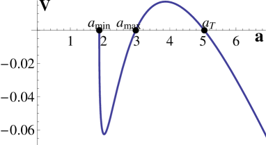
Figure 1: The potential ${V}(a)$ for a matter dominated universe under conditions $g_{m}^{2}=3\mu^{4}\mathcal{E}_{0}$ and $\frac{\mathcal{E}_{0}\rho_{0}}{\mu^{2}}<\frac{9}{8}$. The constants are set as $\mu=1$, $\rho_{0}=0.1$, $g_{m}=5.61249$, and $\mathcal{E}_{0}=10.5$. The radii of the oscillation are $a_{min}=1.87083$ and $a_{max}=2.97382$. The period of this oscillation is $T=18.3324$. The largest root $a_{T}=5.04402$ corresponds to a turning radius of a bouncing universe.

For a general case, we find that there is an oscillating universe if the following conditions are satisfied

$$\mathcal{E}_{0}\rho_{0}<\frac{9}{8}\mu^{2}\;,\quad\quad g_{m}^{-}<g_{m}\leq\sqrt{3\mathcal{E}_{0}}\mu^{2}$$

$$\frac{9}{8}\mu^{2}\leq\mathcal{E}_{0}\rho_{0}<\frac{3}{2}\mu^{2}\;\;,\; g_{m}^{-}<g_{m}<g_{m}^{+},$$ (23)

where $g_{m}^{\pm}$ is defined in Eq. (15). Using above equations, we obtain the allowed region in $(\frac{g_{m}^{2}\rho_{0}}{\mu^{6}},\frac{\mathcal{E}_{0}\rho_{0}}{\mu^{2}})$ plane (Fig. (2)) for an oscillating universe or a bouncing one. The boundaries curves $\Gamma_{\pm}$ are defined as $g_{m}=g_{m}^{\pm}$ (Eq. (15)) and curve $\Gamma$ as $g_{m}=\sqrt{3\mathcal{E}_{0}}\mu^{2}$ (Eq. (13)).

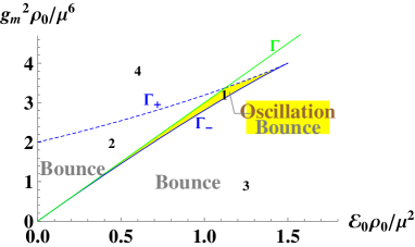
Figure 2: Phase diagram of spacetimes in $(\frac{g_{m}^{2}\rho_{0}}{\mu^{6}},\frac{\mathcal{E}_{0}\rho_{0}}{\mu^{2}})$ plane for a matter dominated universe. An oscillating universe is found in Region 1. A bounce one is found in Regions 1, 2, and 3. The unstable and stable static universes exist on the boundaries $\Gamma_{+}$ and $\Gamma_{-}$, respectively.

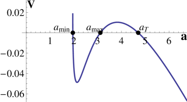
Figure 3: The potential ${V}(a)$ for an oscillating universe or a bouncing one in Region 1 of Fig. (2). The constants are chosen as $\mu=1$, $\rho_{0}=0.1$, $g_{m}=5.75$, and $\mathcal{E}_{0}=11.25$. The radii are $a_{min}=1.96042$, $a_{max}=3.11647$ and $a_{T}=4.70572$. The period of an oscillation is $T=21.9044$.

The period of an oscillation can be calculated through

$$T:=2\int_{a_{min}}^{a_{max}}\frac{da}{\sqrt{-V(a)}}$$ (24)

where $a_{max}$ and $a_{min}$ are the maximum and minimum radius of the oscillating universe.

In Fig. (3), we give the evolutionary curve of the potential with the model parameters satisfying Eq. (III.1.1). From this figure, we find that there is an oscillating universe between $a_{min}$ and $a_{max}$, or a bouncing one in $[a_{T},\infty)$. Therefore, a similar cosmic evolution as shown in Fig. (1) is obtained.

On the $\Gamma_{+}$ curve, the unstable static universe appears. The solution is

$$a_{S}=a_{S}^{+}\;,$$ (25)

with $a_{s}^{+}$ given in Eq. (16), which is a double solution of $V(a)=0$. If $\frac{9}{8}\mu^{2}\leq\mathcal{E}_{0}\rho_{0}<\frac{3}{2}\mu^{2}$, the third root $a_{m}$ is

$$a_{m}=a_{T}^{-}\;,$$ (26)

with $a_{T}^{-}$ given in Eq. (17). In Fig. (4) we plot the evolution of the potential. When $a=a_{S}$, both $V$ and $V^{\prime}$ vanish, but this $a_{S}$ solution is unstable. Therefore, in the $\frac{9}{8}\mu^{2}\leq\mathcal{E}_{0}\rho_{0}<\frac{3}{2}\mu^{2}$ case , the universe can oscillate between $a_{m}$ and $a_{S}$, and it can also evolve directly from $a_{m}$ to $\infty$ or evolve to $\infty$ after some oscillations with no need of quantum tunneling to make it happen. If the universe contracts initially from an infinite scale, it can turn around at $a_{S}$, or pass through $a_{S}$ and bounce at $a_{m}$, then oscillate between $a_{m}$ and $a_{S}$. For the $\mathcal{E}_{0}\rho_{0}<\frac{9}{8}\mu^{2}$ case, if the universe initially evolves from $a_{0}$, it can expand to $a_{S}$, and then it can further expand to infinity or turn around. Once the universe bounces at $a_{S}$ and contracts to $a_{0}$, there will appear a new singularity since at $a_{0}$ the Hubble parameter $H(a_{0})$ is nonzero. That is, when the universe contracts to $a_{0}$ and then expands, it has to evolve discontinuously at $a_{0}$.

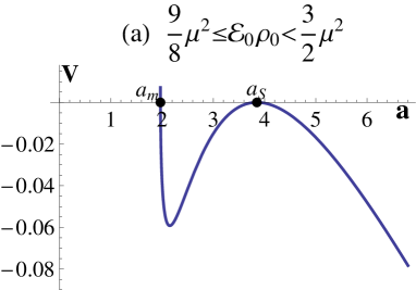
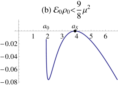
Figure 4: The potential ${V}(a)$ in a matter dominated universe for an unstable static universe (on boundary $\Gamma_{+}$ of Fig. (2)). The constants are chosen $\mu=1$, $\rho_{0}=0.1$, $\mathcal{E}_{0}=11.5$, $g_{m}=5.84184$ (left), and $\mu=1$, $\rho_{0}=0.1$, $\mathcal{E}_{0}=11$, $g_{m}=5.77729$ (right). The radii are $a_{m}=1.96954$, $a_{S}=3.85103$ (left) and $a_{0}=1.90400$, $a_{S}=3.89410$ (right).

A stable static universe or a bouncing one exists on the $\Gamma_{-}$ curve. The stable static solution is

$$a_{S}=a_{S}^{-}$$ (27)

with $a_{s}^{-}$ given in Eq. (16), while the turning radius $a_{T}$ of a bouncing universe is given by

$$a_{T}=a_{T}^{+}$$ (28)

with $a_{T}^{+}$ given in Eq. (17). Fig. (5) gives the potential with model parameter in the $\Gamma_{-}$ curve. There are two solutions ($a_{S}$, $a_{T}$) for $V=0$. At $a=a_{S}$, both $V$ and $V^{\prime}$ are equal to zero and apparently $a=a_{S}$ corresponds to a stable solution. Thus, the universe can stay at this finite radius past-eternally. When $a\geq a_{T}$, $V\leq 0$, which corresponds to a bouncing universe. If the universe stays at $a_{s}$ initially, after a long time, it can quantum mechanically tunnel to the bounce point $a_{T}$ and then expand. If the universe contracts initially from an infinite scale, it will turn around at $a_{T}$.

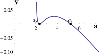
Figure 5: The potential $V(a)$ in a matter dominated universe for a stable static universe and a bouncing one (the ($\Gamma_{-}$) curve of Fig. (2)). The constants are chosen as $\mu=1$, $\rho_{0}=0.1$, $g_{m}=5.75374$, and $\mathcal{E}_{0}=12$. The radius of stable static universe is $a_{S}=2.35114$ and the bounce radius is $a_{T}=5.20431$.

Fig. (6) shows the evolution of the potential ${V}(a)$ with the model parameters in Region 2 of Fig. (2). From this figure, we find that a bouncing universe is obtained since $V\leq 0$ in $a\in[a_{T},\infty)$. In addition, $V\leq 0$ in $a\in[a_{0},a_{m}]$, but $V=0$ occurs only at $a=a_{m}$. Thus, if the universe turns around at $a_{m}$ and contracts to $a_{0}$, as shown in the left panel of Fig. (4), there appears a singularity at $a_{0}$. Of course, if the universe evolves from $a_{0}$ to $a_{m}$ and then quantum tunnels to $a_{T}$ directly, this singularity can be avoided.

Fig. (7) shows the evolution of the potential ${V}(a)$ with the model parameters in Region 3 of Fig. (2). Apparently, a bouncing universe is obtained.

We plot Fig. (8) to give the evolution of the potential with the model parameters in Region 4 of Fig. (2). In this case $V<0$ for $a\geq a_{0}$. Thus an $FS\Rightarrow\infty$ type is obtained.

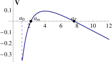
Figure 6: The potential ${V}(a)$ in a matter dominated universe with model parameters in Region 2 of Fig. (2) . The constants are chosen as $\mu=1$, $\rho_{0}=0.1$, $g_{m}=4.47214$, and $\mathcal{E}_{0}=5$. The radii are $a_{0}=1.11803$, $a_{m}=2.23607$, and $a_{T}=7.63441$.

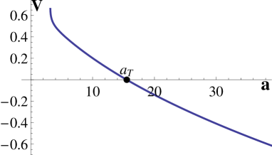
Figure 7: The potential ${V}(a)$ in a matter dominated universe for a bouncing universe (Region 3 of Fig. (2)). The constants are $\mu=1$, $\rho_{0}=0.1$, $g_{m}=3.16228$, and $\mathcal{E}_{0}=10$. The radius is $a_{T}=15.5259$.

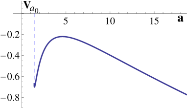
Figure 8: The potential ${V}(a)$ in a matter dominated universe for model parameters in Region 4 of Fig. (2). The constants are chosen as $\mu=1$, $\rho_{0}=0.1$, $g_{m}=7.07107$, and $\mathcal{E}_{0}=10$.

III.1.2 $k=-1$

In this case, the potential is given by

$$V(a)=-1-\frac{1}{3\mu^{2}}\frac{g_{m}}{a}-\frac{\sqrt{2\rho_{0}}}{3\mu^{2}}\sqrt{g_{m}a-\mu^{2}\mathcal{E}_{0}}\;.$$ (29)

Fig. (9) shows the evolution of this potential, from which one can see that, as Fig. (8), the potential $V(a)$ is always negative for $a\geq a_{0}$, which means that the cosmic evolution type is $FS\Rightarrow\infty$.

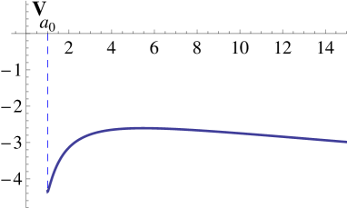
Figure 9: The potential $V(a)$ in a matter dominated universe for the case $\epsilon=+1$, and $k=-1$. The spacetime will always expand. The constants are chosen as $\mu=1$, $\rho_{0}=0.1$, $g_{m}=10$ and $\mathcal{E}_{0}=10$.

III.2 $\epsilon=-1$

In this case, we get

$$V^{\prime}(a)=\frac{1}{3\mu^{2}}\frac{g_{m}}{a^{2}}+\frac{\sqrt{\rho_{0}}}{3\sqrt{2}\mu^{2}}\frac{g_{m}}{\sqrt{g_{m}a-\mu^{2}\mathcal{E}_{0}}}.$$ (30)

Since $V^{\prime}(a)$ is always positive, the potential is an increasing function. Therefore, the cosmic evolution will be simpler than the case of $\epsilon=+1$.

III.2.1 $k=1$

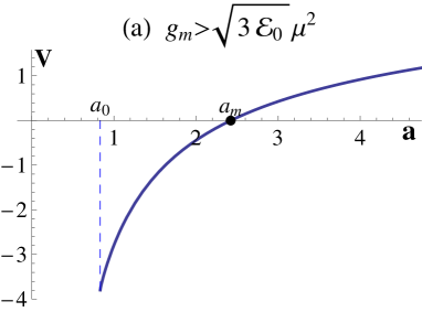
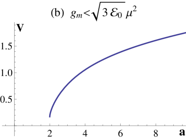
Figure 10: The potential ${V}(a)$ in a matter dominated universe for $\epsilon=-1$ and $k=1$ with $g_{m}>\sqrt{3\mathcal{E}_{0}}\mu^{2}$ (left) and $g_{m}<\sqrt{3\mathcal{E}_{0}}\mu^{2}$ (right). The constants are chosen as $\mu=1$, $\rho_{0}=0.1$, $\mathcal{E}_{0}=10$, $g_{m}=12$ (left) and $\mu=1$, $\rho_{0}=0.1$, $\mathcal{E}_{0}=10$, $g_{m}=5$ (right).

From Fig. (10) one can see there is no solution for $V\leq 0$ if $g_{m}<\sqrt{3\mathcal{E}_{0}}\mu^{2}$. When $g_{m}>\sqrt{3\mathcal{E}_{0}}\mu^{2}$, if $a_{0}\leq a\leq a_{m}$, $V\leq 0$, while $V=0$ occurs only at $a_{m}$. So, the universe can evolve between $a_{0}$ and $a_{m}$, but there is a singularity at $a_{0}$ since $H(a_{0})\neq 0$ at this point, which means that this cosmic evolution type is $FS\Rightarrow FS$. When $g_{m}=\sqrt{3\mathcal{E}_{0}}\mu^{2}$, there is only one point $a=a_{0}$ for $V\leq 0$.

III.2.2 $k=-1$

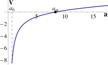
Figure 11: The potential $V(a)$ in a matter dominated universe for the case of $\epsilon=-1$ and $k=-1$. The constants are $\epsilon=-1$, $k=-1$, $\eta=1$, $\mu=1$, $\rho_{0}=0.1$, $\mathcal{E}_{0}=10$, and $g_{m}=15$.

From Fig. (11) we find that, when $a_{0}\leq a\leq a_{m}$, $V\leq 0$. So, a $FS\Rightarrow FS$ type is obtained.

IV The evolution of a radiation-dominated universe in the DGP braneworld

In this section, we discuss the case where the universe is dominated by radiation $(\omega=\frac{1}{3})$. Thus, the cosmic energy density can be expressed as $\rho=\frac{g_{r}}{a^{4}}$, and the potential becomes

$$V(a)=\bigg{(}k-\frac{\epsilon}{3\mu^{2}}\sqrt{2\rho_{0}(g_{r}-\mu^{2}\mathcal{E}_{0})}\bigg{)}-\frac{1}{3\mu^{2}}\frac{g_{r}}{a^{2}}\;.$$ (31)

It is easy to see that $g_{r}\geq\mu^{2}\mathcal{E}_{0}$ is required. As in the previous section, we divide our discussions into two cases: $\epsilon=+1$, and $\epsilon=-1$.

IV.1 $\epsilon=+1$

IV.1.1 $k=1$

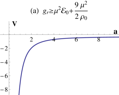
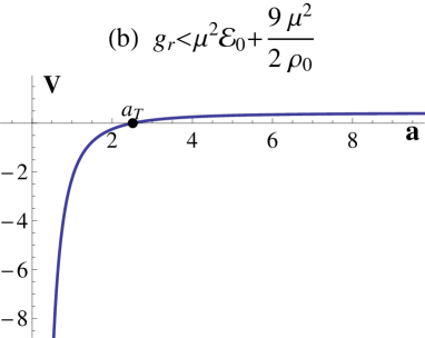
Figure 12: The potential ${V}(a)$ in a radiation dominated universe for $\epsilon=1$ and $k=1$ with $g_{r}\geq\frac{9\mu^{2}}{2\rho_{0}}+\mu^{2}\mathcal{E}_{0}$ (left) and $g_{r}<\frac{9\mu^{2}}{2\rho_{0}}+\mu^{2}\mathcal{E}_{0}$ (right). The constants are chosen as $\mu=1$, $\rho_{0}=0.5$, $\mathcal{E}_{0}=5$, $g_{r}=20$ (left) and $\mu=1$, $\rho_{0}=0.5$, $\mathcal{E}_{0}=5$, $g_{r}=8$ (right). The radius where the universe turns around is $a_{T}=2.51185$.

As shown in Fig. (12), when $g_{r}\geq\frac{9\mu^{2}}{2\rho_{0}}+\mu^{2}\mathcal{E}_{0}$, the potential is always negative and the type of the cosmic evolution is $BB\Rightarrow\infty$ or $\infty\Rightarrow BC$. While, for $\mu^{2}\mathcal{E}_{0}\leq g_{r}<\frac{9\mu^{2}}{2\rho_{0}}+\mu^{2}\mathcal{E}_{0}$, the potential will turn to be positive from negative at the radius $a_{T}$

$$a_{T}=\sqrt{\frac{g_{r}}{3\mu^{2}-\sqrt{2\rho_{0}(g_{r}-\mu^{2}\mathcal{E}_{0})}}}\;.$$ (32)

Thus, the cosmic evolution type is $BB\Rightarrow BC$.

IV.1.2 $k=-1$

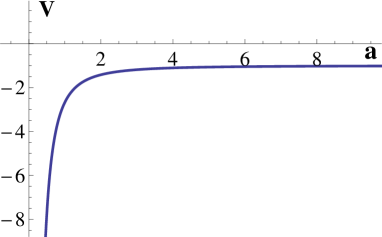
Figure 13: The potential ${V}(a)$ in a radiation dominated universe for $\epsilon=1$ and $k=-1$. The constants are chosen as $\mu=1$, $\rho_{0}=0.5$, $g_{r}=5$, and $\mathcal{E}_{0}=5$.

From Fig. (13) we can see that in this case the potential is always negative and the cosmic evolution type is $BB\Rightarrow\infty$ or $\infty\Rightarrow BC$.

IV.2 $\epsilon=-1$

IV.2.1 $k=1$

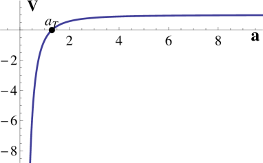
Figure 14: The potential ${V}(a)$ in a radiation dominated universe for $\epsilon=-1$ and $k=1$. The constants are chosen as $\mu=1$, $\rho_{0}=0.5$, $g_{r}=5$, and $\mathcal{E}_{0}=5$. The bounce radius is $a_{T}=1.29099$.

The type of the cosmic evolution now is $BB\Rightarrow BC$ as can be seen from Fig. (14). The turning point is

$$a_{T}=\sqrt{\frac{g_{r}}{3\mu^{2}+\sqrt{2\rho_{0}(g_{r}-\mu^{2}\mathcal{E}_{0})}}}\;.$$ (33)

IV.2.2 $k=-1$

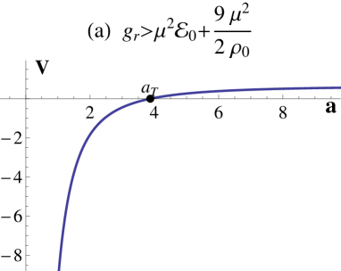
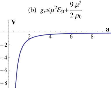
Figure 15: The potential ${V}(a)$ in a radiation dominated universe for $\epsilon=-1$ and $k=-1$ with $g_{r}>\frac{9\mu^{2}}{2\rho_{0}}+\mu^{2}\mathcal{E}_{0}$ (left) and $g_{r}\leq\frac{9\mu^{2}}{2\rho_{0}}+\mu^{2}\mathcal{E}_{0}$ (right). The constants are chosen as $\mu=1$, $\rho_{0}=0.5$, $\mathcal{E}_{0}=5$, $g_{r}=20$ (left) and $\mu=1$, $\rho_{0}=0.5$, $\mathcal{E}_{0}=5$, $g_{r}=8$ (right). The bounce radius is $a_{T}=3.87298$.

From Fig. (15) we obtain that when $g_{r}>\frac{9\mu^{2}}{2\rho_{0}}+\mu^{2}\mathcal{E}_{0}$ the cosmic evolution type is $BB\Rightarrow BC$. The radius where the universe turns to contract is

$$a_{T}=\sqrt{\frac{g_{r}}{-3\mu^{2}+\sqrt{2\rho_{0}(g_{r}-\mu^{2}\mathcal{E}_{0})}}}\;.$$ (34)

When $\mu^{2}\mathcal{E}_{0}\leq g_{r}\leq\frac{9\mu^{2}}{2\rho_{0}}+\mu^{2}\mathcal{E}_{0}$, the cosmic evolution type is $BB\Rightarrow\infty$ or $\infty\Rightarrow BC$ since the potential is always negative.

V The evolution of a vacuum-dominated universe in the DGP braneworld

If the universe is dominated by vacuum energy $(\omega=-1)$, the cosmic energy density is a constant. We denote it by $\rho=g_{v}$, and the potential becomes

$$V(a)=k-\frac{1}{3\mu^{2}}g_{v}a^{2}-\frac{\epsilon}{3\mu^{2}}\sqrt{2\rho_{0}(g_{v}a^{4}-\mu^{2}\mathcal{E}_{0})}\;.$$ (35)

Clearly, $a\geq a_{0}=\sqrt[4]{\frac{\mu^{2}\mathcal{E}_{0}}{g_{v}}}$ is needed, and usually $V(a_{0})\neq 0$ except for the case $k=1$, $\epsilon=-1$ and

$$g_{v}=\frac{9\mu^{2}}{\mathcal{E}_{0}}\;.$$ (36)

V.1 $\epsilon=+1$

V.1.1 $k=1$

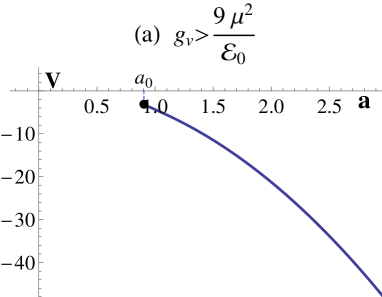
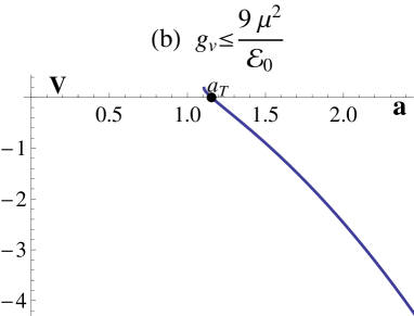
Figure 16: The potential ${V}(a)$ in a vacuum dominated universe for $\epsilon=1$ and $k=1$ with $g_{v}>\frac{9\mu^{2}}{\mathcal{E}_{0}}$ (left) and $g_{v}\leq\frac{9\mu^{2}}{\mathcal{E}_{0}}$ (right). The constants are chosen as $\mu=1$, $\rho_{0}=0.1$, $\mathcal{E}_{0}=10$, $g_{v}=15$ (left) and $\mu=1$, $\rho_{0}=0.1$, $\mathcal{E}_{0}=3$, $g_{v}=2$ (right). And the radius where the universe turns around is $a_{T}=1.1547$.

As plotted in Fig. (16), the potential $V(a)$ is a decreasing function of $a$. If $g_{v}>\frac{9\mu^{2}}{\mathcal{E}_{0}}$, the potential $V(a\geq a_{0})$ is always negative and the type of the cosmic evolution is $FS\Rightarrow\infty$. If $g_{v}\leq\frac{9\mu^{2}}{\mathcal{E}_{0}}$, $V(a_{T})=0$, thus, we get a bouncing universe. The bounce radius is

$$a_{T}=\sqrt{\frac{3g_{v}\mu^{2}-\sqrt{2g_{v}\rho_{0}\mu^{2}(9\mu^{2}-\mathcal{E}_{0}g_{v}+2\mathcal{E}_{0}\rho_{0})}}{g_{v}(g_{v}-2\rho_{o})}}\;.$$ (37)

V.1.2 $k=-1$

We find from Fig. (17) that the cosmic evolution type is $FS\Rightarrow\infty$.

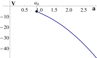
Figure 17: The potential ${V}(a)$ in a vacuum dominated universe for $\epsilon=1$ and $k=-1$. The constants are chosen as $\mu=1$, $\rho_{0}=0.1$, $g_{v}=15$, and $\mathcal{E}_{0}=10$.

V.2 $\epsilon=-1$

V.2.1 $k=1$

In this case, there exists a static universe if $g_{v}$ and other parameters satisfy a relation

$$g_{v}=\frac{9\mu^{2}}{\mathcal{E}_{0}}+2\rho_{0}=g_{v}^{S}\;,$$ (38)

which is obtained by combining $V(a)=0$ and $V^{\prime}(a)=0$. Using the above equation, one can obtain a static state solution

$$a_{S}=\sqrt{\frac{\mathcal{E}_{0}}{3}}\;.$$ (39)

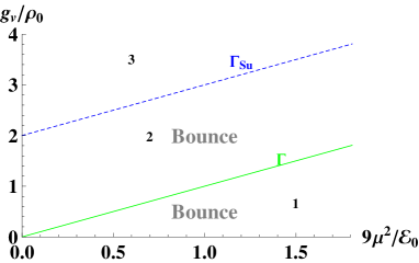
Figure 18: Phase diagram of spacetimes in $(\frac{g_{v}}{\rho_{0}},\frac{9\mu^{2}}{\mathcal{E}_{0}})$ plane for a vacuum dominated universe with $\epsilon=-1$ and $k=1$. A bouncing universe is found in Regions 1, and 2. $a_{0}\Rightarrow\infty$ type of universe are found in Region 3. The unstable and stable static universes exist on the curves $\Gamma_{Su}$ and $\Gamma$, respectively.

Using Eqs. (36, 39), we can depict all cosmic evolution types in the $(\frac{g_{v}}{\rho_{0}},\frac{9\mu^{2}}{\mathcal{E}_{0}})$ plane, which is shown in Fig. (18). On the green line in Fig. (18), which is determined by Eq. (36), we can get a stable static universe with $a_{S}=a_{0}$ and a bouncing one as shown in Fig. (19). Thus, the universe can originate from a stable Einstein static state, which means that the universe stays at this stable state past-eternally and then enters a expanding phase through quantum tunneling. If the universe contracts initially from an infinite scale, it will bounce at $a_{T}$. The radius of the stable static universe is

$$a_{S}=a_{0}=\sqrt{\frac{\mathcal{E}_{0}}{3}},$$ (40)

and the bounce radius is

$$a_{T}=\sqrt{\frac{\mathcal{E}_{0}}{3}+\frac{4\mathcal{E}_{0}^{2}\rho_{0}}{3(9\mu^{2}-2\mathcal{E}_{0}\rho_{0})}}.$$ (41)

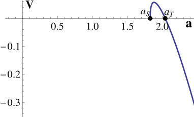
Figure 19: The potential ${V}(a)$ for a stable static universe or a bouncing one in a vacuum dominated phase (the green line of Fig. (18)). The constants are chosen as $\mu=1$, $\rho_{0}=0.05$, $g_{v}=0.9$, and $\mathcal{E}_{0}=10$. The radii are $a_{S}=1.82574$ and $a_{T}=2.04124$.

While, on the blue line of Fig. (18), which is determined by Eq. (38), we obtain an unstable static universe. Its radius is

$$a_{S}=\sqrt{\frac{\mathcal{E}_{0}}{3}}\;.$$ (42)

We plot the effective potential in Fig. (20). From which, one can see that the cosmic evolution type is similar to that shown in the right panel of Fig. (4).

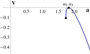
Figure 20: The potential ${V}(a)$ for an unstable static universe in a vacuum dominated phase (the blue line of Fig. (18)). The constants are chosen as $\mu=1$, $\rho_{0}=0.1$, $g_{v}=1.1$, and $\mathcal{E}_{0}=10$. The radii are $a_{0}=1.73640$ and $a_{S}=1.82574$.

Figure 21: The potential ${V}(a)$ in a vacuum dominated universe with the model parameters in Region 1 of Fig. (18). The constants are chosen as $\mu=1$, $\rho_{0}=0.1$, $g_{v}=0.5$. The bounce radius is $a_{T}=3.8941$.

Fig. (21) shows the evolution of the potential ${V}(a)$ with the model parameters in Region 1 of Fig. (18). We find that a bouncing universe is obtained and the bounce radius is

$$a_{T}=\sqrt{\frac{3g_{v}\mu^{2}+\sqrt{2g_{v}\rho_{0}\mu^{2}(9\mu^{2}-\mathcal{E}_{0}g_{v}+2\mathcal{E}_{0}\rho_{0})}}{g_{v}(g_{v}-2\rho_{o})}}\;.$$ (43)

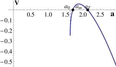
Figure 22: The potential ${V}(a)$ in a vacuum dominated universe with the model parameters in Region 2 of Fig. (18). The constants are chosen as $\mu=1$, $\rho_{0}=0.3$, $g_{v}=1.4$, and $\mathcal{E}_{0}=10$. The radii are $a_{0}=1.63481$, $a_{m}=1.71222$, and $a_{T}=2.13736$.

In Fig. (22), we plot the potential ${V}(a)$ with the model parameters in Region 2 of Fig. (18). A similar result as shown in Fig. (6) is obtained. The expressions for $a_{m}$ and $a_{T}$ are

$$a_{m}=\sqrt{\frac{3g_{v}\mu^{2}-\sqrt{2g_{v}\rho_{0}\mu^{2}(9\mu^{2}-\mathcal{E}_{0}g_{v}+2\mathcal{E}_{0}\rho_{0})}}{g_{v}(g_{v}-2\rho_{o})}}\;,$$ (44)

$$a_{T}=\sqrt{\frac{3g_{v}\mu^{2}+\sqrt{2g_{v}\rho_{0}\mu^{2}(9\mu^{2}-\mathcal{E}_{0}g_{v}+2\mathcal{E}_{0}\rho_{0})}}{g_{v}(g_{v}-2\rho_{o})}}\;.$$ (45)

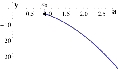
Figure 23: The potential ${V}(a)$ in a vacuum dominated universe with the model parameters in Region 3 of Fig. (18). The constants are chosen as $\mu=1$, $\rho_{0}=0.1$, $g_{v}=15$, and $\mathcal{E}_{0}=10$.

Fig. (23) shows the evolution of the potential ${V}(a)$ with the model parameters in Region 3 of Fig. (18), which corresponds to the cosmic evolution type: $FS\Rightarrow\infty$.

V.2.2 $k=-1$

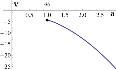
Figure 24: The potential ${V}(a)$ in a vacuum dominated universe with $\epsilon=-1$ and $k=-1$. The constants are chosen as $\mu=1$, $\rho_{0}=0.1$, $g_{v}=10$, and $\mathcal{E}_{0}=10$.

It is easy to see from Fig. (24) that $V(a)$ is always negative. So the cosmic evolution type is $FS\Rightarrow\infty$.

VI Conclusions

In this paper, we have studied all possible cosmic evolutions in the DGP braneworld scenario with a method in which the dynamics of the scale factor is treated like that of a particle in a “potential”. The effect of the dark radiation on the cosmic evolution is considered. By assuming that the cosmic energy component is pressureless matter, radiation or vacuum energy, respectively, we find that, in the matter or vacuum energy dominated case, the universe does not originate from the big bang singularity and its scale factor has a minimum value $a_{0}$. Thus the classical singularity problem can be avoided. However, there may appear a new singularity at $a_{0}$ in the sense that when the universe bounces or contracts to this point and then expands, its evolution will be discontinuous as $H(a_{0})\neq 0$. However, in some circumstances, there exists a stable Einstein static state or a bouncing universe to avoid the new and classical singularities. If the universe is in the Einstein static state initially, it can stay there past-eternally and evolve to the bounce point through quantum tunneling. If the universe contracts initially from an infinite scale, it can turn around at the bounce point and then expand forever. Therefore the cosmic evolution is nonsingular. In addition, in the matter dominated case, there also exists an oscillating universe to avoid the singularity problem as long as the model parameters are in some specific regions (shown in Fig. (2)). If the cosmic scale factor is in the oscillation region initially, the universe may undergo an oscillation. After a number of oscillations, it may evolve to the bounce point through quantum tunneling. In the radiation dominated case, the universe may originate from the big bang singularity, but a bouncing universe which avoids this singularity is also possible.

- (1) S. Perlmutter, et al., Astrophys. J. 517, 565 (1999).
- (2) A. G. Riess, et al., Astrophys. J. 116, 1009 (1998).
- (3) A. G. Riess, et al., Astrophys. J. 607, 665 (2004).
- (4) A. G. Riess et al., Astrophys. J. 659, 98 (2007).
- (5) P. Astier et al., Astron. Astrophys. 447, 31 (2006).
- (6) W. M. Wood-Vasey et al., Astrophys. J. 666, 694 (2007).
- (7) D. Dvali, G. Gabadadze and M. Porrati, Phys. Lett. B 485, 208 (2000).
- (8) C. Deffayet, Phys. Lett. B 502, 199 (2001).
- (9) L. Randall, R. Sundrum, Phys. Rev. Lett. 83, 4690 (1999).
- (10) Y. Shtanov, V. Sahni, Phys. Lett. B 557, 1 (2003).
- (11) A. Lue, Phys. Rept. 423, 1 (2006).
- (12) A. Lue, G.D. Starkman, Phys. Rev. D 70, 101501(R) (2004).
- (13) L.P. Chimento, R. Lazkoz, R. Maartens, I. Quiros, J. Cosmol. Astropart. Phys. 0609, 004 (2006).
- (14) M. Bouhmadi-Lopez, R. Maartens and D. Wands, Phys. Rev. D 70, 123519 (2004).
- (15) R. Cai and H. Zhang, J. Cosmol. Astropart. P. 0408, 017 (2004).
- (16) E. Papantonopoulos and V. Zamarias, J. Cosmol. Astropart. P. 0410, 001 (2004).
- (17) H. Zhang and R. Cai, J. Cosmol. Astropart. P. 0408, 017 (2004).
- (18) H. Zhang and Z. Zhu, Phys. Lett. B 641, 405 (2006).
- (19) S. del Campo, R. Herrera, Phys. Lett. B 653, 122 (2007).
- (20) K. Zhang, P. Wu and H. Yu, Phys. Lett. B 690, 229 (2010).
- (21) V. Sahni and Y. Shtanov, J. Cosmol. Astropart. Phys. 0311, 014 (2003).
- (22) V. Sahni, arXiv: astro-ph/0502032.
- (23) K. Maeda, Y. Misonoh, T. Kobayashi, Phys. Rev. D 82, 064024 (2010).
- (24) K. Maeda, S. Mizuno and T. Torii, Phys. Rev. D 68, 024033 (2003).
- (25) J. B. Hartle, S. W. Hawking, Phys. Rev. D 28, 2960-2975 (1983).
- (26) A. Vilenkin, Phys. Rev. D 30, 509-511 (1984).