Abstract

We review the methods developed for combining the parton shower approximation to QCD with fixed-order perturbation theory, in such a way as to achieve next-to-leading-order (NLO) accuracy for inclusive observables. This has made it possible to generate fully-simulated hadronic final states with the precision and stability of NLO calculations. We explain the underlying theory of the existing methods, MC@NLO and POWHEG, together with their similarities, differences, achievements and limitations. For illustration we mainly compare results on Higgs boson production at the LHC, with particular emphasis on the residual uncertainties arising from the different treatment of effects beyond NLO. We also briefly summarize the difference between these NLO + parton shower methods and matrix-element + parton shower matching, and current efforts to combine the two approaches.

1 Introduction

In the past, parton shower generators and next-to-leading-order (NLO) calculations were seen as complementary approaches to computing hadronic interactions. The former had the more practical purpose of assisting experimental physicists in planning and carrying out experimental analysis. The latter were instead aimed at performing precision tests of perturbative QCD. The simplicity of the framework of fixed-order calculations was in fact required in order to make unbiased comparisons of theoretical calculations and data. After the many tests of QCD carried out at lepton and hadron colliders, convincing evidence was established that perturbative QCD at the NLO level works well, and improves the agreement of theoretical prediction with data. The interest in precise NLO calculations has then shifted in the direction of predicting cross sections and backgrounds for collider processes. In the meantime, a theoretical effort has begun aimed at improving shower generators with the use of more precise matrix elements. This effort has led to two new developments that have had a significant impact on collider phenomenology: matrix-element and shower matching (ME+PS), and NLO calculations interfaced with showers (NLO+PS). The former originated from the so-called CKKW paper [1], and several implementations and variants of the original method have subsequently appeared in the literature (see [2] for a review). In the present review, we focus upon the NLO+PS development, initiated by the MC@NLO paper [3] and followed later by the POWHEG proposal [4]. The aim of these methods was to improve the event generation of a basic process in such a way that NLO accuracy is reached for inclusive observables, while maintaining the leading logarithmic accuracy of the shower approach.

This review is organized as follows. In Section 2 we briefly recall the structure of an NLO calculation, with emphasis on those aspects that are needed for the implementation of NLO+PS generators, and in Section 3 we review the basics of parton showers. In Section 4 we contrast the description of the Sudakov region in fixed-order calculation and in shower algorithms, and specify the requirements for a NLO+PS generator. In these sections, for concreteness, we will always make reference to the simple example of Higgs boson production in gluon fusion in order to clarify the basic concepts.

Sections 5 and 6 illustrate the basics of the MC@NLO and POWHEG methods. The following three sections discuss few issues that are common to both methods. In Section 7 we discuss the use of parton density functions in the NLO+PS framework, and in Section 8, we discuss a commonly used method for the inclusion of spin correlations.

The illustration of the methods given in Sections 5 and 6 are limited for simplicity to cases where there is only one singular region to be considered. There are in essence no conceptual difficulties in dealing with more complex cases, and in Section 9 we give some indications of how this is done.

Section 10 illustrates the role of truncated showers, which were introduced in ref. [4] as a requirement to preserve colour coherence in the POWHEG approach. In this framework, the relation between POWHEG and MC@NLO is also better clarified. This common view of both methods allows one to better understand the origin of differences between them, as discussed in Section 11. In Section 12, the dominant uncertainties in NLO+PS generators are discussed, using again as an example the process of Higgs production via gluon fusion.

In Section 13 we compare the NLO+PS and ME+PS approaches, with the aim of clarifying when either approach should be preferred.

Finally, in Section 14 we briefly summarize the future direction of improvement in the development of NLO+PS generators.

2 Next-to-leading-order calculations in QCD

Next-to-leading-order (NLO) calculations in QCD are used to compute infrared and collinear safe quantities at the one loop level. They considerably reduce the uncertainties of theoretical predictions, and experience from $e^{+}e^{-}$, $ep$ and hadron colliders has shown that they lead to remarkable agreement of theory with data. Since QCD radiation has collinear and infrared divergences, infrared and collinear insensitivity is an unavoidable requirement for an observable to be perturbatively calculable. Thus, fixed-order NLO calculations cannot be used for fully exclusive observables, and are not straightforwardly interfaced to parton shower programs.

A detail explanation of the general structure of an NLO calculation, with particular attention to its use in the context of shower matching, is given in ref. [5]. The reader will also find there references to the most popular subtraction methods for the implementation of QCD NLO corrections. Here we will give an elementary illustration of the typical structure of an NLO calculation, using as an example the gluon fusion production of an on-shell Higgs boson in hadronic collisions. In this example, the Born phase space is characterized by a single variable that can be taken to be equal to the Higgs rapidity $y$. We write the Born cross section as $B\,{\mathrm{d}}\Phi_{\rm B}$, where $B$ is the differential Born cross section, and $\Phi_{\rm B}$ is the Born phase space. In our Higgs example, $B={\mathrm{d}}\sigma_{H}/{\mathrm{d}}y$, and ${\mathrm{d}}\Phi_{\rm B}={\mathrm{d}}y$. The calculation of the NLO cross section for the production process requires the inclusion of the virtual corrections $\hat{V}$ and of a real emission process, with a phase space including one extra parton with respect to the basic process. In our example, the real production process is the production of the Higgs plus one extra gluon. We neglect at this point ${}{{}{{{{{\mathrm{{{}{}{{q}}\mspace{-0.6mu}}}}}}}}}{}{{}{{{{{\mathrm{{{}{}{{g}}\mspace{-0.6mu}}}}}}}}}$, ${}{{}{{{{{\mathrm{{{}{}{{g}}\mspace{-0.6mu}}}}}}}}}{}{{}{{{{{\mathrm{{{}{}{{q}}\mspace{-0.6mu}}}}}}}}}$ and ${}{}{{}{{}{{{{{\mathrm{{{}{}{{\overline{{}{{}{{{{{\mathrm{{{}{}{{q}}\mspace{-0.6mu}}}}}}}}}}}_{{\mspace{1.0mu}}}^{\mspace{1.0mu}{{\raisebox{-1.65764pt}{{${{{\scriptstyle{{{{{\mathrm{{}}}}}}}}}}$}}}}}}\mspace{-0.6mu}}}}}}}}}}{}{{}{{{{{\mathrm{{{}{}{{q}}\mspace{-0.6mu}}}}}}}}}$ processes that arise at NLO, in order to keep our illustration as simple as possible. The real cross section kinematics can be characterized by the Higgs rapidity, as before, and by three variables associated with the emission of an extra parton. We can choose for these variables the cosine of the angle of the emitted parton momentum with respect to the beam direction, its energy and its azimuth, all measured in the Higgs+parton rest frame (i.e. in the partonic centre-of-mass system). We write the real cross section as $R\,{\mathrm{d}}\Phi_{R}$, where ${\mathrm{d}}\Phi_{R}={\mathrm{d}}y\,{\mathrm{d}}\cos\theta\,{\mathrm{d}}E\,{\mathrm{d}}\phi$. We will also write ${\mathrm{d}}\Phi_{R}={\mathrm{d}}\Phi_{\rm B}{\mathrm{d}}\Phi_{\rm rad}$, with ${\mathrm{d}}\Phi_{\rm rad}={\mathrm{d}}\cos\theta\,{\mathrm{d}}E\,{\mathrm{d}}\phi$. We call $\Phi_{\rm rad}$ the radiation phase space. The differential NLO cross section is written schematically as

$${\mathrm{d}}\sigma=\left(B(\Phi_{\rm B})+\hat{V}(\Phi_{\rm B})\right){\mathrm{d}}\Phi_{\rm B}+R(\Phi_{\rm R}){\mathrm{d}}\Phi_{\rm R}\;,$$ (1)

where we have also assumed that all phase space Jacobians needed to reproduce the Lorentz invariant phase space are absorbed into the definition of $B$, $\hat{V}$ and $R$. The virtual cross section $\hat{V}$ (which we assume to be renormalized) has soft and collinear divergences, and must thus be regulated with an infrared cutoff, or by using dimensional regularization. The real cross section also exhibits infrared and ultraviolet divergences after integration over the radiation phase space, such that the full cross section is finite after integration. We have not included in Equation 1 a collinear counterterm, which is needed to remove initial-state collinear singularities, since our aim here is to illustrate the structure of the NLO corrections, rather than give a detail explanation of how they are structured.

Notice that we assume that the real phase space $\Phi_{\rm R}$ can be given as a function of the Born phase space and a radiation phase space, $\Phi_{\rm R}=\Phi_{\rm R}(\Phi_{\rm B},\Phi_{\rm rad})$. This is straightforwardly achieved in our example, but it can be done in general. We will say that $\Phi_{\rm B}$ is the underlying Born configuration of the real phase space. We also require that the mapping $\Phi_{\rm R}(\Phi_{\rm B},\Phi_{\rm rad})$ has the following properties: in the limit in which the radiated parton is soft, $\Phi_{\rm R}$ coincides with $\Phi_{\rm B}$ after removal of the soft parton, and in the limit in which the radiated parton is collinear to another massless parton, $\Phi_{\rm R}$ coincides with $\Phi_{\rm B}$ after merging of the collinear partons. By merging we mean that the two collinear partons are replaced by a single parton, with momentum equal to the sum of the two in case of final state radiation, or equal to the difference of the two in case of initial state radiation. In the Higgs example, the underlying Born configuration is obtained by performing a longitudinal boost to the frame where the Higgs has zero rapidity, and then performing a transverse boost, such that the Higgs transverse momentum vanishes. After that, the inverse of the initial longitudinal boost is applied. In this way the Higgs rapidity remains equal to that in the underlying Born configuration.

The cancellation of soft and collinear singularities in NLO calculations is usually dealt with using the so-called subtraction method. We introduce an auxiliary counterterm $C(\Phi_{\rm R})$, which is required to coincide with the real squared amplitude $R$ in the soft and collinear limits. Assume now that we want to compute an infrared safe observable $O$. Infrared safety requires that

$$O(\Phi_{\rm R}(\Phi_{\rm B},\Phi_{\rm rad}))\to O(\Phi_{\rm B})$$ (2)

in the soft or collinear limit. We can write

$$\langle O\rangle = \int{\mathrm{d}}\Phi_{\rm B}(B(\Phi_{\rm B})+\hat{V}(\Phi_{\rm B}))O(\Phi_{\rm B})+\int{\mathrm{d}}\Phi_{\rm R}\,R(\Phi_{\rm R})O(\Phi_{\rm R})$$ (3)

$$= \int{\mathrm{d}}\Phi_{\rm B}\left[B(\Phi_{\rm B})+V(\Phi_{\rm B})\right]O(\Phi_{\rm B})+\int{\mathrm{d}}\Phi_{\rm R}\,\left[R(\Phi_{\rm R})O(\Phi_{\rm R})-C(\Phi_{\rm R})O(\Phi_{\rm B})\right]$$

where

$$V(\Phi_{\rm B})=\hat{V}(\Phi_{\rm B})+\int{\mathrm{d}}\Phi_{\rm rad}\,C(\Phi_{\rm R}(\Phi_{\rm B},\Phi_{\rm rad}))\;.$$ (4)

The above equations represent schematically the subtraction method in QCD. By a suitable choice of the counterterm $C$, the integral of the radiation variables in Equation 4 can be performed analytically. The soft and collinear divergent terms arising from this integration cancel against those of the virtual term, $\hat{V}$, yielding a finite result $V$ in the sum. At the same time, in Equation 3 the soft and collinear divergences in $R$ cancel, because in the soft or collinear limit $O(\Phi_{\rm R})=O(\Phi_{\rm B})$, and $C$ has the same singularity structure as $R$.

3 Parton shower approximation

The collinear and infrared divergences of QCD are associated with enhanced amplitudes in collinear and soft regions of phase space. These enhancements are manifest in jet production, and in the rapid increase in particle multiplicity in hard scattering processes. They give rise to large logarithmic coefficients in observables that involve widely different scales, for example the jet mass $M$ at a hard process scale $Q\gg M$. The parton shower approximation aims to take the enhanced contributions into account to all orders, neglecting terms with subleading logarithmic or constant coefficients.

We consider first the leading collinear region in which an extra parton is emitted at a small angle by one of the outgoing lines of an $n$-parton process (final-state emission). Here the cross section approximately factorizes in the form

$${\mathrm{d}}\sigma_{n+1}(\Phi_{n+1})={\cal P}(\Phi_{\rm rad})\,{\mathrm{d}}\sigma_{n}(\Phi_{n})\,{\mathrm{d}}\Phi_{\rm rad}$$ (5)

and ${\mathrm{d}}\Phi_{n+1}={\mathrm{d}}\Phi_{n}\,{\mathrm{d}}\Phi_{\rm rad}$. The function ${\cal P}$ depends on the type of emitting and emitted partons. In the notation of the previous Section, if the $n$-parton process is the Born process, we have $\Phi_{n}=\Phi_{\rm B}$, $\Phi_{n+1}=\Phi_{\rm R}$, and ${\cal P}(\Phi_{\rm rad})\,B(\Phi_{\rm B})\equiv R^{({\rm MC})}(\Phi_{\rm R})$ is an approximation to $R(\Phi_{\rm R})$ in the near-collinear region. In this region it is convenient to parametrize the phase space $\Phi_{\rm rad}$ in terms of a hardness scale $q$, for example the transverse momentum $p_{\rm T}$ relative to the emitter, the fraction of longitudinal momentum $z$ of the emitter after the emission, and the azimuthal angle of splitting, $\phi$. Then

$${\cal P}(\Phi_{\rm rad})\,{\mathrm{d}}\Phi_{\rm rad}\approx\frac{\alpha_{\rm S}(q)}{\pi}\,\frac{{\mathrm{d}}q}{q}\,P(z,\phi)\,{\mathrm{d}}z\frac{{\mathrm{d}}\phi}{2\pi}\,,$$ (6)

where $P(z,\phi)$ is the relevant (DGLAP) splitting function, which in practice is averaged over the azimuthal angle and simply written as $P(z)$. The collinear divergence is regulated with a cutoff, $q>Q_{0}$. Emissions with $q<Q_{0}$ are said to be unresolvable. Emissions with small momentum fractions $z$ are also unresolvable. Depending on the definition of the scale $q$, the cutoff on $z$ is some function $z_{0}(q,Q_{0})$.

Equations 5 and 6 provide the basis of an iterative scheme for summing collinear-enhanced contributions to all orders. Each parton participating in a hard process can emit at scales $q$ up to order $Q$. The probability of an emission in an interval between $q+dq$ and $q$ is given by Equation 6. It follows that the probability of no resolvable emissions between scales $q_{1}$ and $q_{2}<q_{1}$ is given by

$$\Delta_{\rm S}(q_{1},q_{2})=\exp\left[-\int_{q_{2}}^{q_{1}}\frac{\alpha_{\rm S}(q)}{\pi}\frac{{\mathrm{d}}q}{q}\int_{z_{0}}^{1}P(z)\,{\mathrm{d}}z\right]\,.$$ (7)

This function is known as the Sudakov form factor.

We have justified Equation 7 using unitarity, i.e. the conservation of probability. We now remark that relying solely upon field theory would lead to the same conclusions. In other words, it can be proven that the inclusion of all logarithmically enhanced virtual corrections in a shower process amounts to the inclusion of running couplings at each splitting vertex, evaluated at a scale of the order of the virtuality of the incoming parton, supplemented by the insertion of a Sudakov form factor on each internal line, having as argument its virtuality. The result satisfies unitarity, which we do expect, since field theory must satisfy unitarity. We can say, more specifically, that logarithmic singularities must cancel in inclusive quantities, thanks to the Kinoshita-Lee-Nauenberg (KLN) theorem [6, 7], which in turn is a consequence of unitarity. Thus we expect all singularities to cancel order by order in perturbation theory, and in fact we see that by expanding the Sudakov form factor in Equation 7 at order $\alpha_{\rm S}$ we do get a term that cancels exactly the integral of the real diagram describing the splitting process in the collinear approximation, given by Equations 5 and 6.

In a parton shower event generator, multiple emissions are generated by the Monte Carlo method. Given the initial scale $Q$, the scale of the first emission is found by solving the equation $\Delta_{\rm S}(Q,q_{1})=R_{1}$, where $R_{1}$ is a pseudorandom number uniform on the interval [0,1]. The next emission is at $q_{2}<q_{1}$ where $\Delta_{\rm S}(q_{1},q_{2})=R_{2}$, and so on, until the chosen scale falls below the cutoff $Q_{0}$. The emitted partons can themselves emit in the same way. In this way each outgoing parton from the hard process is converted into a shower of partons at the cutoff scale $Q_{0}$. Below this scale the running coupling becomes large and colour confinement ensures that the parton showers are converted into jets of hadrons. Perturbation theory is not applicable to this process and one has to resort to hadronization models, which fall outside the scope of the present article (for a review see [2]). One important feature of the hadronization process, observed experimentally and built into the models, should however be noted here, namely its locality: the flow of energy-momentum and flavour in the parton showers is preserved, up to power-suppressed corrections, in the resulting hadron jets. This justifies the comparison of results in perturbative QCD with data on hadronic final states.

Shower Monte Carlo generators also treat initial-state radiation in the collinear approximation, but the kinematics are slightly different: a parton from an incoming hadron beam starts at a low scale with its momentum along the beam direction and recoils with a more spacelike four-momentum after each emission, eventually reaching the hard process scale $q\sim Q$ with a significant transverse momentum. For technical reasons it is more convenient to treat this in the opposite direction, evolving incoming partons from the hard scale down to the hadronic scale, where they are matched to the parton distributions of the incoming hadrons.

In order to arrive at a formula for the backward splitting probability in initial-state radiation, we begin by writing the forward splitting probability in the form

$${\cal P}(\Phi_{\rm rad}){\mathrm{d}}\Phi_{\rm rad}\approx\frac{R^{\rm MC}_{n+1}}{R_{n}^{\rm MC}}{\mathrm{d}}\Phi_{\rm rad}\,,$$ (8)

where $R^{\rm MC}_{n+1}$ and $R_{n}^{\rm MC}$ are the $n+1$ and $n$ body cross section in the MC approximation, in the singular limit. This formula can be immediately generalized to initial-state radiation, the only difference being due to the fact that the ratio of parton density functions in $R^{\rm MC}_{n+1}/R^{\rm MC}_{n}$ does not cancel as in final-state radiation, leading to the formula

$${\cal P}^{({\rm ISR})}(\Phi_{\rm rad}){\mathrm{d}}\Phi_{\rm rad}\approx\frac{\alpha_{\rm S}(q)}{\pi}\,\frac{{\mathrm{d}}q}{q}\,P(z)\frac{f(x/z,q)}{f(x,q)}\,{\mathrm{d}}z\frac{{\mathrm{d}}\phi}{2\pi}\,,$$ (9)

which is Sjöstrand’s formula for backward evolution [8] in initial state radiation.

Collinear parton emission can be treated at the cross-section level, as in Equation 5, because an emission cannot be collinear with more than one hard parton. This is not the case for soft gluon emission, which occurs coherently from different partons and so should be treated at the amplitude level. Two approximate showering schemes have been developed to take account of soft gluon interference. In angular-ordered showering, the scale variable $q$ is defined so that successive parton emissions are at decreasing angles. The separate colour charges of a pair of partons in the shower with opening angle $\theta$ can be resolved by soft gluons emitted at smaller angles, $\theta^{\prime}<\theta$, so this emission is treated incoherently. On the other hand, when $\theta^{\prime}>\theta$ the partons are not resolved and they emit as a single object with the colour charge of their parent parton. Therefore this emission is treated as coming from the parent, corresponding to angular ordering of successive emissions, as shown in Figure 1.

Figure 1: Angular ordering of coherent soft gluon radiation ($\theta^{\prime}>\theta$).

The other method for treating soft gluon coherence is dipole showering [9]. Instead of sequential splitting of one parton into two, pairs of partons are treated as dipole sources for gluon emission, which splits one dipole into two. This is valid in the large-$N$ approximation, where $N$ is the number of colours. Some subleading colour effects are included by matching the resulting cross sections to the parton splitting functions in collinear regions.

4 The Sudakov region

The most visible difference between an NLO result and the output of a parton shower is the structure of the so-called Sudakov region, i.e. the region where radiation with low energy and transverse momentum is important. In the example of Higgs production, this is the region where the transverse momentum of the Higgs is much smaller than its mass. The ${\cal O}(\alpha_{\rm S}^{3})$ result for this quantity diverges as $\log(p_{\rm T}/M_{{}{{}{{{{{\mathrm{{{}{}{{H}}\mspace{-0.6mu}}}}}}}}}})/p_{\rm T}$ in the $p_{\rm T}\to 0$ limit. However, the integral of the $p_{\rm T}$ distribution from zero to any finite value is finite. In other words, one should imagine that a contribution formed by a negative $\delta$ function with an infinite coefficient is located at $p_{\rm T}$ equal to zero, and that it cancels the divergent contribution arising from the real emission cross section.

In the small $p_{\rm T}$ region, perturbation theory is not reliable any more, and one needs to resum the large logarithms of $p_{\rm T}$ to all orders in perturbation theory. In the leading logarithmic approximation, this distribution is dominated by recoil of the Higgs against the hardest emission. The shower Monte Carlo algorithm yields for the hardest emission the cross section

$$\frac{{\mathrm{d}}\sigma^{({\rm MC})}}{{\mathrm{d}}y\,{\mathrm{d}}p_{\rm T}}=\frac{{\mathrm{d}}\sigma^{({\rm B})}}{{\mathrm{d}}y}\delta(p_{\rm T})\Delta(Q_{0})+\Delta(p_{\rm T})\frac{{\mathrm{d}}\sigma^{({\rm MC})}}{{\mathrm{d}}y\,{\mathrm{d}}p_{\rm T}}\;,\quad\Delta(p_{\rm T})=\exp\left[-\int_{p_{\rm T}}^{Q}\frac{\frac{{\mathrm{d}}\sigma^{({\rm MC})}}{{\mathrm{d}}y\,{\mathrm{d}}p_{\rm T}^{\prime}}}{\frac{{\mathrm{d}}\sigma^{({\rm B})}}{{\mathrm{d}}y}}{\mathrm{d}}p_{\rm T}^{\prime}\right]\;.$$ (10)

The factor $\Delta(p_{\rm T})$ arises from the product of the two $\Delta_{\rm S}(Q,p_{\rm T})$ Sudakov form factors, associated with the radiation from each initial line, in the notation of Equation 7. Here $Q$ is the hard process scale, of the order of $M_{{}{{}{{{{{\mathrm{{{}{}{{H}}\mspace{-0.6mu}}}}}}}}}}$ in this case, and $\sigma^{({\rm MC})}$ denotes the shower Monte Carlo approximation for the real emission cross section. If we assume that the shower algorithm is ordered in $p_{\rm T}$, Equation 10 is a simple consequence of the shower formula, since it corresponds to the generation of the first emission by the algorithm. It can be shown, however, that the formula also holds for angular ordered showers, where the hardest emission is not necessarily the first [4]. We notice that the shower unitarity relation holds

$$\int_{0}^{Q}\left[\delta(p_{\rm T})\Delta(Q_{0})+\frac{\int_{Q_{0}}^{Q}\Delta(p_{\rm T})\frac{{\mathrm{d}}\sigma^{({\rm MC})}}{dy{\mathrm{d}}p_{\rm T}}}{\frac{{\mathrm{d}}\sigma^{({\rm B})}}{{\mathrm{d}}y}}\right]{\mathrm{d}}p_{\rm T}=\Delta(Q_{0})+\int_{Q_{0}}^{Q}\frac{{\mathrm{d}}\Delta(p_{\rm T})}{{\mathrm{d}}p_{\rm T}}{\mathrm{d}}p_{\rm T}=\Delta(Q)=1$$ (11)

so that

$$\int_{0}^{Q}{\mathrm{d}}p_{\rm T}\frac{{\mathrm{d}}\sigma^{({\rm MC})}}{{\mathrm{d}}y{\mathrm{d}}p_{\rm T}}=\frac{{\mathrm{d}}\sigma^{({\rm B})}}{{\mathrm{d}}y}.$$ (12)

This relation is independent of the particular form of $\sigma^{({\rm MC})}$.

A shower Monte Carlo program alone will generate a transverse momentum distribution that is accurate only for small transverse momenta, since ${\mathrm{d}}\sigma^{({\rm MC})}$ is reliable only in the collinear approximation. For small transverse momenta, however, rather than having the singular behaviour of an NLO calculation, it is well behaved, with the Sudakov form factor damping the small $p_{\rm T}$ singularity of the tree level result. Many event generators are capable of adding a matrix-element correction (MEC), such that for large transverse momentum the shower result matches the fixed-order result [10]. This is achieved, in essence, by replacing $\sigma^{({\rm MC})}$ with $\sigma^{({\rm NLO})}$ in Equation 10. Assuming, for the moment, that we are dealing with a shower algorithm ordered in transverse momentum, the generation of the first emission in MEC is given by

$${\mathrm{d}}\sigma^{({\rm MEC})}=B{\mathrm{d}}\Phi_{\rm B}\left[\Delta(Q_{0})+\Delta(p_{\rm T})\frac{R}{B}{\mathrm{d}}\Phi_{\rm rad}\right],\quad\Delta(p_{\rm T})=\exp\left[-\int\frac{R}{B}\delta(p_{\rm T}(\Phi_{\rm R})-p_{\rm T}){\mathrm{d}}\Phi_{\rm rad}\right]\;.$$ (13)

The notation used in Equation 13 deserves some explanation. We write in a compact notation a fully differential cross section that can have different final states as a single formula. The first term in the square bracket represents the production of an event with the Born kinematics, and phase space $\Phi_{\rm B}$. In the Higgs example, it represents a Higgs boson with zero transverse momentum. The second term represents the full real process, with production of a Higgs and a parton, balanced in transverse momentum. The above formula represents the probability that either event is produced.

The shower unitarity Equation 11 is then written in the general form

$$\Delta(Q_{0})+\int\Delta(p_{\rm T})\frac{R}{B}{\mathrm{d}}\Phi_{\rm rad}=1\,,$$ (14)

where it is intended that the ${\mathrm{d}}\Phi_{\rm rad}$ integration is limited to the region where $p_{\rm T}(\Phi_{\rm R})\geq Q_{0}$.

In Figure 2

Figure 2: Transverse momentum distribution of the Higgs at NLO, in a shower algorithm, and in a MEC shower.

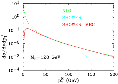
we give a pictorial representation of the distribution of the transverse momentum of the Higgs boson at fixed rapidity at NLO order (i.e. ${\cal O}(\alpha_{\rm S}^{3})$), from the shower algorithm, and from a MEC shower algorithm. For the NLO result, one should imagine that the NLO curve diverges at small $p_{\rm T}$ up to a tiny cutoff, and that a tiny bin with a very large, negative value is located at $p_{\rm T}=0$. The resummation of collinear and soft singularities performed by the shower algorithm using the exact real emission cross section starts to differ from the LO one at $p_{\rm T}$ around $40$ GeV, and for smaller $p_{\rm T}$ it tames the divergence of the NLO cross section. The shower approximation has the same behaviour for moderate to small $p_{\rm T}$, but it drops rapidly as $p_{\rm T}$ approaches the maximum scale of radiation allowed by the shower algorithm (an exact implementation of Equation 10 would imply that the cross section vanishes exactly for $p_{\rm T}\geq Q$. Subsequent emissions in the shower process will tend to smear the region of $p_{\rm T}\approx Q$). The area under the two shower curves equals the Born cross section.

The main objective of a NLO+PS implementation is to improve the shower approximation, in such away that it achieves NLO accuracy for inclusive quantities. Thus, referring to Figure 2, we would expect that the Higgs transverse momentum distribution in an NLO+PS approach should have the smooth shape of the Shower and MEC approaches at small $p_{\rm T}^{{}{{}{{{{{\mathrm{{{}{}{{H}}\mspace{-0.6mu}}}}}}}}}}$, should match (up to even higher order terms) the NLO calculation at large $p_{\rm T}^{{}{{}{{{{{\mathrm{{{}{}{{H}}\mspace{-0.6mu}}}}}}}}}}$, and should have the total area of the curve equal to ${\mathrm{d}}\sigma^{\rm NLO}/{\mathrm{d}}y$. In other words

$$\frac{{\mathrm{d}}\sigma^{\rm NLO+PS}}{{\mathrm{d}}y\,{\mathrm{d}}p_{\rm T}^{{}{{}{{{{{\mathrm{{{}{}{{H}}\mspace{-0.6mu}}}}}}}}}}}=K(y,p_{\rm T}^{{}{{}{{{{{\mathrm{{{}{}{{H}}\mspace{-0.6mu}}}}}}}}}})\frac{{\mathrm{d}}\sigma^{\rm MEC}}{{\mathrm{d}}y\,{\mathrm{d}}p_{\rm T}^{{}{{}{{{{{\mathrm{{{}{}{{H}}\mspace{-0.6mu}}}}}}}}}}}\,.$$ (15)

where $K(y,p_{\rm T}^{{}{{}{{{{{\mathrm{{{}{}{{H}}\mspace{-0.6mu}}}}}}}}}})=1+\alpha_{\rm S}k(y,p_{\rm T}^{{}{{}{{{{{\mathrm{{{}{}{{H}}\mspace{-0.6mu}}}}}}}}}})$ is a rapidity and transverse momentum dependent $K$-factor. We require $K$ to be smooth for small $p_{\rm T}^{{}{{}{{{{{\mathrm{{{}{}{{H}}\mspace{-0.6mu}}}}}}}}}}$, so that the smooth shape of the shower and MEC approaches is preserved, and to be such that

$$\int{\mathrm{d}}p_{\rm T}^{{}{{}{{{{{\mathrm{{{}{}{{H}}\mspace{-0.6mu}}}}}}}}}}\frac{{\mathrm{d}}\sigma^{\rm NLO+PS}}{{\mathrm{d}}y\,{\mathrm{d}}p_{\rm T}^{{}{{}{{{{{\mathrm{{{}{}{{H}}\mspace{-0.6mu}}}}}}}}}}}=\frac{{\mathrm{d}}\sigma^{({\rm NLO})}}{{\mathrm{d}}y}\,.$$ (16)

For example, we could require

$$K(y,p_{\rm T}^{{}{{}{{{{{\mathrm{{{}{}{{H}}\mspace{-0.6mu}}}}}}}}}})=K(y)=\frac{\frac{{\mathrm{d}}\sigma^{({\rm NLO})}}{{\mathrm{d}}y}}{\frac{{\mathrm{d}}\sigma^{({\rm B})}}{{\mathrm{d}}y}}\,,$$ (17)

which, using the fact that

$$\int{\mathrm{d}}p_{\rm T}^{{}{{}{{{{{\mathrm{{{}{}{{H}}\mspace{-0.6mu}}}}}}}}}}\frac{{\mathrm{d}}\sigma^{\rm MEC}}{{\mathrm{d}}y\,{\mathrm{d}}p_{\rm T}^{{}{{}{{{{{\mathrm{{{}{}{{H}}\mspace{-0.6mu}}}}}}}}}}}=\frac{{\mathrm{d}}\sigma^{({\rm B})}}{{\mathrm{d}}y}\,,$$ (18)

satisfies Equation 16. With this choice, the large transverse momentum tail of the distribution differs from the pure NLO result by terms suppressed by a further power of $\alpha_{\rm S}$, i.e. terms of NNLO order. But this does not spoil NLO accuracy, and it is therefore allowed. Alternatively, the $K$ factor may also have some transverse momentum dependence, such that the corresponding curve in Figure 2 would be above the MEC result for $p_{\rm T}\ll M_{{}{{}{{{{{\mathrm{{{}{}{{H}}\mspace{-0.6mu}}}}}}}}}}$, but would approach it for larger transverse momenta. This NNLO ambiguity in the definition of an NLO+PS generator is unavoidable, and it should thus be kept in mind that different NLO+PS generators, besides differing because of different renormalization and factorization scale choices, and different shower algorithms, may also differ because of this.

5 MC@NLO

In the parton shower Monte Carlo approach, one starts from the Born cross section $B(\Phi_{\rm B})$ and adds higher-order corrections in the shower approximation. If one started instead from the NLO cross section, there would be double counting because the showers would add terms that are already present in the NLO result. The aim of the MC@NLO scheme is to remove from the NLO expressions those terms that will be generated by the parton showers. This is achieved by modifying the subtraction terms of the NLO calculation. The method was worked out in detail in [3] and applied there to vector boson pair production, then extended to heavy quark pair production in [11]. In [12] the decay angular correlations in these processes were added. Single top quark production processes were implemented in [13, 14, 15]. The present version [16, 17] also includes the single and associated production of Higgs and vector bosons. All these processes are implemented for hadron-hadron collisions. Heavy quark photoproduction has been considered in [18]. The aMC@NLO project, developing a fully automated NLO event generator based on the MC@NLO scheme, with loop corrections from MadLoop [19] using the OPP method [20, 21], has provided results on a range of more complex processes of interest [22, 23, 24]. A variant of the MC@NLO approach has been implemented within the Sherpa event generator [25, 26].

Referring to Section 3, one can see that two types of NLO terms are generated by parton showering and need to be removed from the NLO calculation.

1. A resolvable real emission gives rise to a positive term of the form in Equation 5, which has to be subtracted from the corresponding term in Equation 1. That is, one must replace $R(\Phi_{\rm B},\Phi_{\rm rad})$ by $R(\Phi_{\rm B},\Phi_{\rm rad})-R^{({\rm MC})}(\Phi_{\rm B},\Phi_{\rm rad})$.

2. In addition, expansion of the Sudakov form factor for no resolvable emission, $\Delta_{\rm S}(Q,Q_{0})$in Equation 7, to first order gives a negative term which is the integral of $-R^{({\rm MC})}(\Phi_{\rm B},\Phi_{\rm rad})$ over the real emission phase space $\Phi_{\rm rad}$.

Thus in place of Equation 1 one should start the parton shower Monte Carlo from the modified NLO cross section

$${\mathrm{d}}\sigma_{\rm mod} = \left(B(\Phi_{\rm B})+\hat{V}(\Phi_{\rm B})+\int R^{({\rm MC})}(\Phi_{\rm B},\Phi_{\rm rad}){\mathrm{d}}\Phi_{\rm rad}\right){\mathrm{d}}\Phi_{\rm B}$$ (19)

$$+ \Bigl{(}R(\Phi_{\rm B},\Phi_{\rm rad})-R^{({\rm MC})}(\Phi_{\rm B},\Phi_{\rm rad})\Bigr{)}{\mathrm{d}}\Phi_{\rm B}\,{\mathrm{d}}\Phi_{\rm rad}\;,$$

where the extra terms are understood to be summed over all coloured external lines of the Born process. By comparison with Equations 3 and 4, one can see that this amounts to a modification of the counterterms $C(\Phi_{\rm R})$ in the subtraction method. It is clear that, upon integrating over the real emission phase space $\Phi_{\rm rad}$, Equation 19 reproduces the equivalent NLO cross section in Equation 1. However, it should be emphasised that ${\mathrm{d}}\sigma_{\rm mod}$ as it stands does not represent a physical differential cross section: for example, the distribution of real emissions is completely wrong and must be supplemented by the emissions generated by a parton shower generator. Furthermore Equation 19 is specific to a particular generator, represented by the label (MC). For each shower generator, one must calculate analytically exactly what the program does at relative order $\alpha_{\rm S}$ and modify the NLO counterterms accordingly. At present there are complete MC@NLO versions [16, 27] for the HERWIG [28, 29] and Herwig++ [30, 31] event generators, while aMC@NLO is also available [23, 32] for PYTHIA [33] with virtuality-ordered parton showering.

In the analytical calculation of the modified counterterms, to avoid the useless generation of unresolvable emissions and cancelling virtual corrections, the resolution cutoff $Q_{0}$ should be set to zero. This has the effect of cancelling the divergences of the pure NLO counterterms, provided the Monte Carlo distribution $R^{({\rm MC})}$ is accurate in the soft and collinear regions. In collinear regions, factorization of the cross section according to Equation 6 is exact and so the cancellation of collinear singularities is guaranteed. In soft, non-collinear regions, the azimuthal averaging of the splitting functions and the angular-ordering treatment of coherence used in the Monte Carlo mean that the cancellation of soft divergences occurs after integration over angles and not point-by-point. Smoothing functions are therefore introduced to match the MC and NLO expressions in these regions. This is not a problem as physical observables are insensitive to the angles of soft gluon emission. In addition, the factorization of colour structure in Equation 6 does not hold in general in soft, non-collinear regions, so there may be colour-suppressed contributions with non-cancelling sub-leading divergences, which give rise to power-suppressed corrections after smoothing and do not affect the NLO accuracy of predictions. A proof of this point is given in Appendix A. For technical details, see the Appendices of refs. [3, 11].

The cancellation of divergences makes it possible to prepare separate samples of Born-like and real emission configurations for processing by the shower generator, known as $\mathbb{S}$ events and $\mathbb{H}$ events respectively, each with finite weights equal to the relevant coefficient in Equation 19. This is in contrast to a pure NLO calculation, where the positive divergences of the real emission distribution are cancelled by negatively divergent contributions in the Born phase space. The $\mathbb{S}$ and $\mathbb{H}$ events can be unweighted, if desired, by accepting them in proportion to their weights before showering. However, these weights are not guaranteed to be positive, so some configurations generate counter-events that have to be subtracted rather than added in histograms. As can be seen from Equation 19, provided the Monte Carlo is close to the true emission distribution in the important regions, the counter-events tend to be a small fraction of $\mathbb{H}$ events that serve to correct predictions to the NLO level.

In Section 4 we claimed that a NLO+PS generator should spread the NLO $K$ factor over a certain region of the transverse momentum distribution of the hardest radiation. If we dropped the second and third term in the first line of Equation 19, the MC@NLO result would approach that of a MEC accurate Monte Carlo, with the ${\mathbb{S}}$ events being just the shower events, and the ${\mathbb{H}}$ events correcting the shower hardest emission at large transverse momenta, in order to match the tree-level result. The integrated cross section would be near the Born cross section. In fact, the second line of Equation 19 gives only a minor contribution to the integral, since it is non-vanishing only in the large transverse momentum region where the collinear approximation differs substantially from the tree-level matrix element. By including the full round bracket on the first line of Equation 19, we increase only the ${\mathbb{S}}$ contribution by a $K$ factor depending on the Born kinematics $\Phi_{\rm B}$. We thus see that in the MC@NLO case the $K$ factor acts uniformly over the $p_{\rm T}$ region that is dominated by ${\mathbb{S}}$ events, which typically extends out to $p_{\rm T}$ values of the order of the hard scale of the process in question, while the region of harder emissions is not affected by it.

The practical implementation of the MC@NLO method proceeds as follows. The NLO part first performs the integrations necessary to determine the weights of the $\mathbb{S}$ events and then generates the $\mathbb{S}$ and $\mathbb{H}$ events (i.e. Born-like and Born+one-parton configurations, respectively) to serve as the starting-points of the corresponding MC generator. These may remain weighted or can be unweighted as described above. For the purposes of parton showering and hadronization, each event has to be assigned a unique colour flow, which corresponds to the large-$N_{c}$ limit of QCD, where $N_{c}$ is the number of colours. Therefore a colour flow is selected according to their relative probabilities in the large-$N_{c}$ limit of the corresponding Born or real emission matrix element. However, it should be emphasised that the sum of all colour flows reproduces the full NLO result, including all subleading $N_{c}$ dependence. Each coloured external line of the event can then be processed by the shower generator in the normal way. In particular, there is no restriction that shower emissions from $\mathbb{H}$ events should be softer than the extra parton emitted at the NLO level, because the weights of those events are computed assuming unrestricted showering. However, $\mathbb{H}$ events are not singular in the collinear and soft regions, and thus their contribution to those regions is phase-space suppressed, so that the cross section for producing events in which the shower generates radiation much harder than that generated in the $\mathbb{H}$ configuration is power suppressed.

Figure 3: Transverse momentum (upper left plot) and rapidity (upper right) distributions of the top quark, and transverse momentum (lower right) and relative azimuth (lower left) distributions of the $t\bar{t}$ pair at the LHC (14 TeV), obtained at NLO, with HERWIG, and with MC@NLO. Figures from [11].

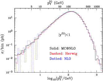
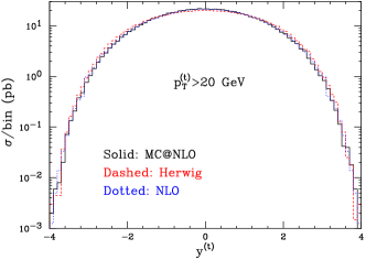
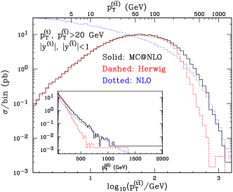
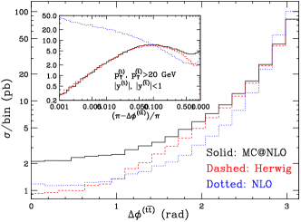
Figure 3 shows some MC@NLO results on top quark pair production at the LHC, compared with those obtained at NLO and with HERWIG. The MC@NLO and HERWIG results, but not of course the NLO ones, include parton showering and hadronization. For ease of comparison, the HERWIG results have been rescaled by $\sigma_{\rm NLO}/\sigma_{\rm LO}$, so that all plots have the same normalization.

For the inclusive transverse momentum and rapidity distributions of the top quark, higher-order corrections tend to have a global effect without causing much change of shape in the distributions, and consequently the results of all three approaches are similar. It should be noted, however, that the MC@NLO results are more stable than pure NLO with respect to statistical fluctuations. This is due to the absence of divergences in the weights within the $\mathbb{S}$ and $\mathbb{H}$ event samples separately, rather than cancellation of oppositely divergent weights between the two samples. Thus it can happen that a given statistically significance is achieved more quickly, in spite of the extra computation involved in parton showering.

For quantities sensitive to correlations between the top quark and antiquark, differences are more apparent. The MC@NLO prediction for the transverse momentum distribution of the pair follows the NLO result at high $p_{\rm T}$, while the HERWIG distribution, generated by parton showering alone, falls off rapidly at values above the top quark mass. At low $p_{\rm T}$ the opposite is the case, as $\mathbb{S}$ events dominate and the distribution is controlled by parton showering, so that MC@NLO agrees with the (rescaled) Monte Carlo prediction. On the other hand, both NLO and HERWIG fall below the MC@NLO prediction at low values of the azimuthal angle between the pair, where both single hard and multiple soft emissions contribute.

6 POWHEG

The basic idea in POWHEG (the acronym stands for Positive Weight Hardest Emission Generator) is to generate the hardest radiation first, and then feed the event to any shower generator for subsequent, softer radiation. In shower generators ordered in transverse momenta, the hardest emission is always the first, and in this case POWHEG simply replaces the hardest emission with its own, NLO accurate emission. In angular ordered showers, the hardest radiation may not be the first, and, as shown in ref. [4], the inclusion of so-called “truncated showers”, to be discussed in Section 10, is needed to restore soft coherence in these cases. In POWHEG events can be produced with positive (constant) weight. Furthermore, since the algorithm does not depend upon a particular parton shower program, the POWHEG output can be easily interfaced to any modern shower generator that is capable of handling user processes (typically those that comply with the Les Houches Interface for User’s Processes [34]).

The first proofs of concept of POWHEG were the implementation of $Z$ pair production in hadronic collisions [35], followed by the implementation of heavy flavour production [36]. The method was described in great details in ref. [5]. Drell-Yan vector boson production [37], Higgs boson production via gluon fusion [38] and single-top production [39] were soon implemented. In ref. [40], a package for the implementation of POWHEG for generic processes was presented, called the POWHEG BOX, that allows one, given the NLO matrix elements for a process, to build its POWHEG implementation automatically. Several processes have been implemented within this framework [41, 42, 43, 44, 45, 46, 47, 48, 49]. Notably, in refs. [50, 51, 52, 53], the POWHEG BOX was used in conjunction with the HELAC-NLO package [54] for the computation of processes of considerable complexity.

Independent POWHEG efforts have also being pursued by the Herwig++ [30] and by the Sherpa [55] collaborations. Besides having implemented several processes in the POWHEG framework [56, 57, 58, 59, 60], the Herwig++ team has also developed the implementation of truncated showers, needed to recover soft coherence when interfacing POWHEG with an angular ordered parton shower generator. The Sherpa collaboration has developed a partially automated procedure for the implementation of POWHEG in [61].

As already discussed in Section 4, the MEC approximation in the shower formalism reproduces the NLO cross section at large transverse momenta. Multiplying the MEC cross section for the hardest emission by a $K$ factor that is a function of the underlying Born kinematics (the Higgs rapidity in our Higgs example), it is possible to achieve NLO accuracy for inclusive quantities. To be more precise, let us write the shower algorithm formula for the generation of the largest $p_{\rm T}$ radiation in the shower-MEC approximation

$$\frac{{\mathrm{d}}\sigma^{({\rm MEC})}}{{\mathrm{d}}y{\mathrm{d}}p_{\rm T}} = {\mathrm{d}}\Phi_{\rm B}B\left[\delta(p_{\rm T})\Delta(Q_{0})+\Delta(p_{\rm T})\frac{R}{B}{\mathrm{d}}\Phi_{\rm rad}\right],$$ (20)

$$\Delta(p_{\rm T}) = \exp\left[-\int\frac{R}{B}{\mathrm{d}}\Phi_{\rm rad}\theta(p_{\rm T}(\Phi_{\rm rad})-p_{\rm T})\right]\;.$$

We now claim that formula 20 achieves NLO accuracy if we replace the prefactor

$${\mathrm{d}}\Phi_{\rm B}B\to{\mathrm{d}}\Phi_{\rm B}\bar{B}\,,\quad\quad\bar{B}=B+V+\int R{\mathrm{d}}\Phi_{\rm rad}\,.$$ (21)

Before proving this result, we first introduce the POWHEG procedure in its full generality. One splits the real cross section into two components

$$R=R^{\rm S}+R^{\rm F},$$ (22)

where $R^{\rm F}$ is regular in the small $p_{\rm T}$ region, and $R^{\rm S}$ embodies all the singularities. The POWHEG formula for the generation of the hardest radiation is

$${\mathrm{d}}\sigma={\mathrm{d}}\Phi_{\rm B}\bar{B}^{\rm S}\left[\Delta_{\rm S}(Q_{0})+\Delta_{\rm S}(p_{\rm T})\frac{R^{\rm S}}{B}{\mathrm{d}}\Phi_{\rm rad}\right]+R^{\rm F}{\mathrm{d}}\Phi_{\rm R},$$ (23)

$$\bar{B}^{\rm S}=B+\hat{V}+\int R^{\rm S}\,d\Phi_{\rm rad}\,,\quad\Delta_{\rm S}(p_{\rm T})=\exp\left[-\int\frac{R^{\rm S}}{B}{\mathrm{d}}\Phi_{\rm rad}\theta(p_{\rm T}(\Phi_{\rm rad})-p_{\rm T})\right]\;.$$ (24)

A simple way to achieve the $R^{\rm S}$-$R^{\rm F}$ separation is to choose

$$R^{\rm S}=\frac{h^{2}}{h^{2}+p_{\rm T}^{2}}\,,\quad R^{\rm F}=\frac{p_{\rm T}^{2}}{h^{2}+p_{\rm T}^{2}}\;.$$ (25)

With this separation, taking $h\to\infty$, $R^{\rm F}$ vanishes, and one recovers the case of Equation 20 with the replacement Equation 21.

In POWHEG, the hardest radiation is generated using Equation 23. This event is then fed to a shower Monte Carlo, which is required not to generate any radiation with larger transverse momentum. Because of the presence of the cutoff $Q_{0}$, a small fraction of events without radiation will also be generated. In this case, also the shower will not generate radiation.

We now demonstrate that the POWHEG formula, Equation 23, yields NLO accuracy when applied to IR-safe observables. We call ${\cal O}$ such an observable. First of all, we notice that further showering, beyond the hardest radiation, must affect the shape variable only to a subleading level, and it is thus enough to prove NLO accuracy for the POWHEG generated event. We have

$$\langle{\cal O}\rangle = \frac{1}{\sigma}\Bigg{\{}\int d\Phi_{\rm B}\bar{B}^{\rm S}\left[{\cal O}(\Phi_{\rm B})\Delta_{\rm S}(Q_{0})+\int\Delta_{\rm S}(p_{\rm T})\frac{R^{\rm S}}{B}{\cal O}(\Phi_{\rm R})\,{\mathrm{d}}\Phi_{\rm rad}\right]$$ (26)

$$+\int{\cal O}(\Phi_{\rm R})R^{\rm F}{\mathrm{d}}\Phi_{\rm R}\Bigg{\}}\,$$

From Equation 26, by adding and subtracting the same quantity, we obtain immediately

$$\langle{\cal O}\rangle = \frac{1}{\sigma}\Bigg{\{}\int d\Phi_{\rm B}\bar{B}^{\rm S}\left[{\cal O}(\Phi_{\rm B})\Delta_{\rm S}(Q_{0})+\int\Delta_{\rm S}(p_{\rm T})\frac{R^{\rm S}}{B}{\cal O}(\Phi_{\rm B})\,{\mathrm{d}}\Phi_{\rm rad}\right]$$

$$+\int d\Phi_{\rm R}\bar{B}^{\rm S}\Delta_{\rm S}(p_{\rm T})\frac{R^{\rm S}}{B}\left({\cal O}(\Phi_{\rm R})-{\cal O}(\Phi_{\rm B})\right)\,+\int{\cal O}(\Phi_{\rm R})R^{\rm F}{\mathrm{d}}\Phi_{\rm R}\Bigg{\}}\,.$$

$$= \frac{1}{\sigma}\left\{\int d\Phi_{\rm B}\bar{B}^{\rm S}{\cal O}(\Phi_{\rm B})+\int d\Phi_{\rm R}R^{\rm S}\left({\cal O}(\Phi_{\rm R})-{\cal O}(\Phi_{\rm B})\right)\,+\int{\cal O}(\Phi_{\rm R})R^{\rm F}{\mathrm{d}}\Phi_{\rm R}\right\}\,.$$

By unitarity (see Equation 14), the expression in the square bracket in the first line of Equation 6 has been replaced by ${\cal O}(\Phi_{\rm B})$ in the last equality. Furthermore, another simplification has been applied in the last equality, which follows from the fact that the first term in the middle line of Equation 6 is finite (since the factor ${\cal O}(\Phi_{\rm R})-{\cal O}(\Phi_{\rm B})$ damps the singular region) and of NLO order. One can then drop the $\bar{B}^{\rm S}/B$ ratio and the Sudakov form factor in this term, since they both differ from unity by higher-order terms, which lead to corrections of order higher than NLO. Finally, replacing $\bar{B}^{\rm S}$ with its explicit expression, we get

$$\langle{\cal O}\rangle = \frac{1}{\sigma}\Bigg{\{}\int d\Phi_{\rm B}\left[B+V+\int R^{\rm S}{\mathrm{d}}\Phi_{\rm rad}\right]{\cal O}(\Phi_{\rm B})+\int d\Phi_{\rm R}R^{\rm S}\left({\cal O}(\Phi_{\rm R})-{\cal O}(\Phi_{\rm B})\right)$$ (28)

$$+\int{\cal O}(\Phi_{\rm R})R^{\rm F}{\mathrm{d}}\Phi_{\rm R}\Bigg{\}}\,\,$$

$$= \frac{1}{\sigma}\left\{\int d\Phi_{\rm B}[B+V]{\cal O}(\Phi_{\rm B})+\int d\Phi_{\rm R}[R^{\rm S}+R^{\rm F}]{\cal O}(\Phi_{\rm R})\right\}\,,$$

which concludes our proof. In the last line we assume that some sort of infrared regulator is applied to the virtual term and to the integral of the real term, so that infrared cancellation takes place as usual for infrared insensitive quantities. As we will see in the following, further showering is forced to be softer than the hardest radiation in POWHEG, so that IR-safe observables are affected by it only at a subleading level.

It is interesting to ask ourselves what happens if we take the limit $h\to 0$. It turns out that the $\bar{B}^{\rm S}$ function will develop a negative infinity, since the integration of $R^{\rm S}$ has a positive soft-collinear singularities that cancels an analogous negative singularity in the virtual term. By gradually reducing $R^{\rm S}$, the negative infinity in $V$ will be gradually exposed. It is also clear that the transverse momentum distribution will approach more and more the NLO result, and the proof of NLO accuracy that we have just given guarantees that the NLO result is recovered. From this discussion, it becomes clear that $h$ should be such that the nice shape of the $p_{\rm T}$ distribution in the region of the resummation should not be spoiled, i.e. $h$ cannot be taken too small.

The POWHEG generated event is fed to a general-purpose shower Monte Carlo (SMC) such as HERWIG or PYTHIA for the generation of the rest of the parton shower and hadronization. Care must be taken, however, that the SMC should not generate radiation with transverse momenta larger than that of the initial parton. An SMC complying with the Les Houches Interface for User Processes (LHIUP from now on) can be easily instructed to do so, just by setting the common block variable scalup to the transverse momentum of the POWHEG generated radiation. When we talk about the transverse momentum generated by the SMC, we mean here either the transverse momentum with respect to the beam axis, for initial state radiation partons, or the transverse momentum with respect to a final state parton, if the emission is from a final state parton. Observe that, in the case of no radiation (i.e. the event consists of the Higgs boson alone), scalup has to be set to such a small value that further radiation from the SMC is essentially prohibited. In the following we will refer to the event generated by POWHEG as the Les Houches event (LHE), precisely because POWHEG passes the event to the SMC by using the LHIUP.

We will not try to illustrate here how the POWHEG event is generated in practice. The interested reader can look at the first POWHEG implementation [35], or at the general POWHEG papers [5, 40] for details. We only note here that, besides generating the event kinematics, one must also assign colour to the final state partons, according to the LHIUP convention. The only requirement for the correctness of the POWHEG procedure is that colour assignment should be at least as accurate as in a shower Monte Carlo. In the POWHEG BOX, for example, a process-specific routine assigns the colour to the underlying Born configuration. This is generally done in the large $N_{\rm c}$ limit, but subleading colour connections may also be included, if desired. The POWHEG BOX then assigns colour to the generated hardest emission configuration, assuming the large-$N_{\rm c}$ limit colour assignment in collinear radiation that is used in parton shower algorithms.

7 Use of parton density functions in NLO+PS generators

In order to claim NLO accuracy, an NLO+PS generator must make some use of NLO accurate parton densitites. In both MC@NLO and POWHEG the generation process begins with the calculation of an inclusive cross section, which is given by the two terms in round bracket in Equation 19 for MC@NLO, and by the calculation of $\bar{B}$ and $R^{\rm F}$ (see Equation 23) in POWHEG. The $\bar{B}$ function in POWHEG, as well as the term in round bracket in the first line of Equation 19 in MC@NLO, must be computed using NLO accurate parton density functions (PDFs). Strictly speaking, this is not needed for the $R^{\rm F}$ term in POWHEG and for the ${\mathbb{H}}$ events in MC@NLO (i.e. for the second line of Equation 19), although in practice NLO PDFs are also alway used there. Parton densities also play a role in the generation of radiation via backward evolution in MC@NLO. In POWHEG they play a role in the generation of the hardest radiation for initial-state radiation, and subsequently in the SMC that takes care of the rest of the radiation. In these steps, NLO PDFs are not needed. The key observation needed to justify the above statements is that NLO PDFs are needed when they multiply a contribution to the cross section that is of leading order. For example, in Higgs production, NLO PDFs are needed in the contributions to the cross section that start at order $\alpha_{\rm S}^{2}$. This is because NLO and LO PDFs differ by terms of order $\alpha_{\rm S}$, which multiplied by a term of order $\alpha_{\rm S}^{2}$ lead a term of NLO accuracy. In the NLO+PS generators this is only the case for the ${\mathbb{S}}$ and $S$ cross sections in MC@NLO and POWHEG, respectively. In MC@NLO it is in general preferred to run the shower stage using the MC internal PDF’s, although a user can optionally use the same NLO PDFs used in the NLO calculation. In POWHEG, the generation of the hardest radiation is usually performed using the NLO PDFs, although other choices are possible.

8 Spin correlations in decays

Basic processes that include narrow resonance decays can be dealt with in a standard way in both MC@NLO and POWHEG, considering the decay as part of the Born process. Thus, for example, for ${}{{}{{{{{\mathrm{{{}{}{{Z}}\mspace{-0.6mu}}}}}}}}}$ production, one can consider ${}{{}{{{{{\mathrm{{{}{}{{q}}\mspace{-0.6mu}}}}}}}}}{}{}{{}{{}{{{{{\mathrm{{{}{}{{\overline{{}{{}{{{{{\mathrm{{{}{}{{q}}\mspace{-0.6mu}}}}}}}}}}}_{{\mspace{1.0mu}}}^{\mspace{1.0mu}{{\raisebox{-1.65764pt}{{${{{\scriptstyle{{{{{\mathrm{{}}}}}}}}}}$}}}}}}\mspace{-0.6mu}}}}}}}}}}\to{}{{}{{{{{\mathrm{{{}{}{{Z}}\mspace{-0.6mu}}}}}}}}}\to{}{{}{{{{{\mathrm{{{}{}{{{}{{}{{{{{\mathrm{{{}{}{}\mspace{-0.6mu}}}}}}}}}}^{-}}\mspace{-0.6mu}}}}}}}}}{}{{}{{{{{\mathrm{{{}{}{{{}{{}{{{{{\mathrm{{{}{}{}\mspace{-0.6mu}}}}}}}}}}^{+}}\mspace{-0.6mu}}}}}}}}}$. In this way, the angular correlation of the final state decay products with the rest of the event are accounted for correctly.

In the case of the production of spinless particles, as in Higgs production, it is always more convenient to treat the decay at a later stage, since the production formulae are simpler for the undecayed object, and the whole process implementation becomes simpler. One first generates the resonance, and then replaces it with its decay products, distributed isotropically in its rest frame. The same procedure can also be applied to the production and decay of resonances with spin, but, in doing so, one loses spin correlations.

In ref. [12], a method for the inclusion of spin correlations in the decay of resonances in Monte Carlos, applicable also to NLO+PS implementations, has been introduced. In essence, the method works as follows. The MC@NLO framework generates an event to be passed to the shower Monte Carlo, which is simply the partonic Born configuration in the case of ${\mathbb{S}}$ events, or the Born configuration plus the radiation of one parton in ${\mathbb{H}}$ events. The idea is essentially to complete the partonic event by letting the heavy resonance decay and weighting the angular distribution of its decay products according to the corresponding tree-level matrix element. This procedure certainly captures correctly the Born level angular distribution, and, for hard radiation, also the correct correlation when an associated hard jet is produced. The same procedure can be applied to the POWHEG case. In POWHEG, most events include the hardest radiation. In this case the correlation is retained even if the radiated parton is near the collinear region, or very soft. It should be kept in mind, however, that the procedure of ref. [12] does not include the full NLO correction to correlations, since the spin dependence of the virtual corrections is not fully accounted for.

In final state resonance decays into coloured particles, like ${}{{}{{{{{\mathrm{{{}{}{{q}}\mspace{-0.6mu}}}}}}}}}{}{}{{}{{}{{{{{\mathrm{{{}{}{{\overline{{}{{}{{{{{\mathrm{{{}{}{{q}}\mspace{-0.6mu}}}}}}}}}}}_{{\mspace{1.0mu}}}^{\mspace{1.0mu}{{\raisebox{-1.65764pt}{{${{{\scriptstyle{{{{{\mathrm{{}}}}}}}}}}$}}}}}}\mspace{-0.6mu}}}}}}}}}}\to{}{{}{{{{{\mathrm{{{}{}{{Z}}\mspace{-0.6mu}}}}}}}}}\to{}{{}{{{{{\mathrm{{{}{}{{q}}\mspace{-0.6mu}}}}}}}}}{}{}{{}{{}{{{{{\mathrm{{{}{}{{\overline{{}{{}{{{{{\mathrm{{{}{}{{q}}\mspace{-0.6mu}}}}}}}}}}}_{{\mspace{1.0mu}}}^{\mspace{1.0mu}{{\raisebox{-1.65764pt}{{${{{\scriptstyle{{{{{\mathrm{{}}}}}}}}}}$}}}}}}\mspace{-0.6mu}}}}}}}}}}$, or top production and decays, the same method can be, and in fact is, used. Chain decays, such as ${}{{}{{{{{\mathrm{{{}{}{{t}}\mspace{-0.6mu}}}}}}}}}\to{}{{}{{{{{\mathrm{{{}{}{{W}}\mspace{-0.6mu}}}}}}}}}{}{{}{{{{{\mathrm{{{}{}{{b}}\mspace{-0.6mu}}}}}}}}}\to{}{{}{{{{{\mathrm{{{}{}{{q}}\mspace{-0.6mu}}}}}}}}}{}{}{{}{{}{{{{{\mathrm{{{}{}{{\overline{{}{{}{{{{{\mathrm{{{}{}{{q}}\mspace{-0.6mu}}}}}}}}}}}_{{\mspace{1.0mu}}}^{\mspace{1.0mu}{{\raisebox{-1.65764pt}{{${{{\scriptstyle{{{{{\mathrm{{}}}}}}}}}}$}}}}}}\mspace{-0.6mu}}}}}}}}}}$, are also handled. However, next-to-leading corrections to the decay process are not included. Thus, for example, in the implementation of heavy flavour production in MC@NLO and POWHEG, the top decay is only handled at the leading-order level, and only at this level are spin correlations accounted for correctly.

9 MC@NLO and POWHEG for complex processes

The discussion given so far has focussed upon a relatively simple process, where only initial-state collinear radiation has to be dealt with. In general, final-state massless partons may also be present, and should be properly considered. Typically, processes like single top production, or Higgs production via vector boson fusion, have final-state light partons that can emit collinear radiation. In processes of associated jet production, like vector boson plus one jet production, or dijet production, one has the further complication that the Born cross section itself is divergent, unless some transverse momentum cut on the jet kinematics is imposed. All these issue add practical complexity to the NLO+PS implementation. However, no conceptual complexity arises: the same method used in the simplest cases can be applied in the most complex ones. The key observation is that the real cross section can be split into a sum of contributions with specific flavour structure that are singular in one collinear region only. One writes

$$R=\sum_{\alpha}R^{\alpha}$$ (29)

where each $\alpha$ labels a particular flavour structure and a singular region of the real amplitude, and the $R^{\alpha}$ is required to be singular only in the corresponding region. Considering, for example, $Z+{\rm jet}$ production, the real-emission flavour structure ${}{}{{}{{}{{{{{\mathrm{{{}{}{{\overline{{}{{}{{{{{\mathrm{{{}{}{{q}}\mspace{-0.6mu}}}}}}}}}}}_{{\mspace{1.0mu}}}^{\mspace{1.0mu}{{\raisebox{-1.65764pt}{{${{{\scriptstyle{{{{{\mathrm{{}}}}}}}}}}$}}}}}}\mspace{-0.6mu}}}}}}}}}}{}{{}{{{{{\mathrm{{{}{}{{q}}\mspace{-0.6mu}}}}}}}}}\to Z{}{{}{{{{{\mathrm{{{}{}{{g}}\mspace{-0.6mu}}}}}}}}}{}{{}{{{{{\mathrm{{{}{}{{g}}\mspace{-0.6mu}}}}}}}}}$ has the following singular configurations: the first emitted gluon may have vanishing transverse momentum (i.e. it is soft or collinear to either of the initial-state partons), the second emitted gluon may have vanishing transverse momentum, or the two emitted gluons may have small relative angle. The full cross section for the ${}{}{{}{{}{{{{{\mathrm{{{}{}{{\overline{{}{{}{{{{{\mathrm{{{}{}{{q}}\mspace{-0.6mu}}}}}}}}}}}_{{\mspace{1.0mu}}}^{\mspace{1.0mu}{{\raisebox{-1.65764pt}{{${{{\scriptstyle{{{{{\mathrm{{}}}}}}}}}}$}}}}}}\mspace{-0.6mu}}}}}}}}}}{}{{}{{{{{\mathrm{{{}{}{{q}}\mspace{-0.6mu}}}}}}}}}\to Z{}{{}{{{{{\mathrm{{{}{}{{g}}\mspace{-0.6mu}}}}}}}}}{}{{}{{{{{\mathrm{{{}{}{{g}}\mspace{-0.6mu}}}}}}}}}$ process may be written as

$$R=R_{1}+R_{2}+R_{3}\,,\quad R_{i}=R\frac{{\cal D}_{i}}{{\cal D}_{1}+{\cal D}_{2}+{\cal D}_{3}},{\cal D}_{i}=\left(\frac{1}{p_{T}^{(i)}}\right)^{q}\,,$$ (30)

with $q\geq 2$, where $p_{T}^{(1)}$ is the transverse momentum of the first gluon, $p_{T}^{(2)}$ is the transverse momentum of the second gluon, and $p_{T}^{(3)}$ is the relative transverse momentum of the two final state gluons. It is clear that $R_{1}$ is singular only when the first gluon is collinear to either initial-state parton, $R_{2}$ is singular only when the second gluon is collinear to either initial-state parton, and $R_{3}$ is singular only if the two final-state gluons are collinear to each other. Notice also that the soft singularities are partitioned among the different collinear regions, but that in all cases nothing is omitted, since the sum of the three contribution yields the total real amplitude by construction. Both POWHEG and MC@NLO adopt a similar separation of the collinear regions. In the computation of the ${\mathbb{S}}$ events in MC@NLO, the third term on the first line of Equation 19 should include all contributions arising from the shower, i.e. initial-state radiation and final-state radiation. The term on the second line of Equation 19 is instead split into all singular components of $R$, and each component is accompanied by the corresponding MC component. Thus, for example, the final-state radiation contribution will have the structure

$$R_{3}(\Phi_{\rm B},\Phi_{\rm rad})-R^{({\rm MC})}_{\rm fsr}(\Phi_{\rm B},\Phi_{\rm rad})\,,$$ (31)

where $\Phi_{\rm rad}$ refer here to the final-state radiation variables, and $R^{({\rm MC})}_{\rm fsr}$ refers to the Monte Carlo implementation of the final-state splitting process. Notice that the NLO and MC terms in Equation 31 must be expressed in terms of the same variables, including appropriate Jacobian factors.

In POWHEG, in the case of multiple singular regions, one must first of all define the appropriate $\bar{B}$ function as

$$\bar{B}^{\rm S}_{f_{b}}=B_{f_{b}}+V_{f_{b}}+\sum_{\alpha\in\{\alpha|f_{b}\}}\int R^{\rm S}_{\alpha}d\Phi_{\rm rad}^{(\alpha)}\;.$$ (32)

Here $f_{b}$ represents a specific Born flavour configuration, and the notation $\{\alpha|f_{b}\}$ stands for all $\alpha$ such that $R^{\rm S}_{\alpha}$ has $f_{b}$ as flavour of the underlying Born configuration. Notice that the mapping of $\Phi_{\rm B}$ and $\Phi_{\rm rad}$ into the full real phase space also depends upon the particular singular contribution that we are considering, and the superscript $\alpha$ on $\Phi_{\rm rad}$ is there to remind us of this fact. We can think of the $\bar{B}^{\rm S}_{f_{b}}$ as the inclusive NLO cross section at fixed underlying Born flavour $f_{b}$ and kinematics $\Phi_{\rm B}$. Of course, the definition of the underlying Born structure also depends upon the separation of the real cross section $R$ into the singular components $R^{\rm S}_{\alpha}$, and upon the mapping that is used in a particular singular region for constructing the real phase space out of the underlying Born phase space and the radiation variables. A detailed description of the decomposition Equation 29 and of the mappings is given in ref. [5].

The generation of radiation in POWHEG, once the underlying Born kinematics and flavour structure have been generated, is obtained using as Sudakov form factor the expression

$$\Delta^{f_{b}}(p_{\rm T},\Phi_{\rm B})=\exp\left\{-\sum_{\alpha\in\{\alpha|f_{b}\}}\int\frac{{\mathrm{d}}\Phi_{\rm rad}^{(\alpha)}R^{\rm S}_{\alpha}\;\theta(k_{\rm T}^{(\alpha)}(\Phi_{\rm R}^{(\alpha)})-p_{\rm T})}{B^{f_{b}}}\right\}\;.$$ (33)

Again, the sum in the exponent is over all $\alpha$ such that $R^{\rm S}_{\alpha}$ has $f_{b}$ as the flavour of the underlying Born configuration, and the integral is performed at fixed underlying Born configuration. The function $k_{\rm T}^{(\alpha)}$ is the radiation transverse momentum, i.e. the transverse momentum of the radiated parton in initial-state radiation, and the transverse momentum of the radiated parton relative to a final-state parton in final-state radiation, and for this reason it depends upon the singular region under consideration. The Sudakov form factor in Equation 33 is the probability that no radiation, either initial- or final-state, from any of the final-state partons, has $k_{\rm T}$ larger than $p_{\rm T}$. In practice, in order to generate the radiation, the full Sudakov form factor is decomposed in the product of Sudakov form factors for each $R^{\rm S}_{\alpha}$ contribution. According to standard Monte Carlo methods, the generation of $p_{\rm T}$ according to Equation 33) can be performed by generating a $p_{\rm T}$ using each Sudakov form factor, and picking the largest.

The generation of the contribution of the non-singular $R^{\rm F}$ terms does not present any particular problem.

10 Truncated showers

In angular-ordered showers, like those in HERWIG and Herwig++, the hardest emission during the shower development may not necessarily be the first in the shower chain. As seen in Section 3, angular ordering allows softer, larger-angle emission to take place earlier in the shower development, in order to account for coherent soft gluon emission from a bunch of collinear partons. These soft, large-angle emissions see the bunch of collinear emitting partons as a single coherent colour source, its colour being that of the parent parton of the bunch. This is why the shower can treat these emissions as if they were coming from a single parton. In ref. [4], it was shown that even in the case of angular-ordered showers, the hardest parton emission is described, up to subleading corrections, by the equation

$${\mathrm{d}}\sigma = B\,{\mathrm{d}}\Phi_{\rm B}\left[\Delta(Q_{0})+\Delta(p_{\rm T})\frac{R^{({\rm MC})}}{B}{\mathrm{d}}\Phi_{\rm rad}\right],$$

$$\Delta(p_{\rm T}) = \exp\left[-\int\frac{R^{({\rm MC})}}{B}\;\delta(p_{\rm T}(\Phi_{\rm R})-p_{\rm T})\;{\mathrm{d}}\Phi_{\rm rad}\right],$$ (34)

which has the same form as Equation 13. It was thus suggested that the Herwig shower was equivalent to a shower initiated by Equation 10), which we call in the following the initial process, with the remaining radiation provided as follows:

I A shower initiated at an angle determined by the underlying Born configuration of the initial process, stopping at an angle equal to that of the emission in the initial process , vetoing radiation harder (i.e. with larger transverse momentum) than the initial-process radiation. This shower was called a vetoed truncated shower in ref. [4].

II All partons produced in the initial process are allowed to radiate with standard angular-order initial conditions, but radiation with transverse momentum larger than that of the initial process is vetoed.

The vetoed truncated shower described in item I is needed in order to supply the soft, coherent radiation that can be emitted at large angles by the splitting partons associated with the hardest emission. An angular-ordered shower algorithm generates this radiation first, so the hardest emission may take place later in the shower. If instead the shower is started with the hardest emission, this coherent radiation must be added explicitly.

In ref. [4] it was proposed to implement a positive weights NLO+PS generator by generating the initial process with the POWHEG method, and to complete the shower according to the prescriptions I and II. It was also pointed out that vetoed-truncated showers are not really specific requirements of POWHEG, but that they also appear naturally in the CKKW matrix-element to shower matching (ME+PS). In ref. [62], an implementation of CKKW matching using truncated showers has been proposed in the Herwig++ framework. An implementation of truncated showers in the Sherpa framework has been proposed in [63]. However, since Sherpa uses a transverse momentum ordered dipole shower, one can no longer claim that truncated showers are needed there to restore the coherence of soft emission.

11 POWHEG and MC@NLO comparisons

In the present section we compare and contrast the MC@NLO and POWHEG methods. As discussed in Section 10, it was shown in ref. [4] that the Herwig shower could be replaced by a shower where the hardest emission is generated first, and that the hardest emission, up to subleading corrections, is described by Equation 10. It then follows that, up to their nominal accuracy, we can identify the MC@NLO prescription with a POWHEG implementation having $R^{\rm S}=R^{({\rm MC})}$, where the $\mathbb{S}$ and the $\mathbb{H}$ events in MC@NLO are identified with the S and F events respectively in POWHEG. This reasoning provides an alternative to the proof in ref. [3] of the correctness of the MC@NLO procedure by showing that it is equivalent to a POWHEG approach, so that the proof of NLO accuracy for inclusive observables used for POWHEG also applies. Furthermore, it allows us to better understand the similarities and differences between the two approaches. As will be made clear, they can mostly be traced back to differences between $R^{\rm S}$ and $R^{({\rm MC})}$.

Detailed comparisons of MC@NLO and POWHEG were carried out in refs. [35, 36, 38, 37, 39]. Remarkable agreement was found for inclusive quantities, i.e. quantities that are inclusive in the hardest jet being radiated. Discrepancies were found in the kinematics of the hardest jet, especially for processes with a very large NLO $K$ factor, like Higgs production. We will focus now upon these distributions, bearing in mind that all the discrepancies reflect differences in the estimation of corrections that are beyond the formal accuracy of the two approaches.

We begin by showing the transverse momentum distribution of the Higgs in the left plot of Figure 4.

Figure 4: Transverse momentum distribution of the Higgs (left plot) and distribution of the rapidity distance between the Higgs and the hardest jet, obtained with HERWIG, with MC@NLO and with MC@NLO with the the NLO corrections to the ${\mathbb{S}}$ events switched off. For comparison, the POWHEG+PYTHIA result is also shown for the $h=\infty$ and $h=100~{}$GeV value of the parameter of eq. 25.

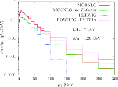
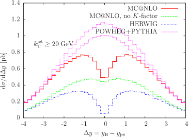
The POWHEG and MC@NLO predictions agree for moderate transverse momenta. For large transverse momenta POWHEG gives a larger results, with the upper POWHEG prediction (corresponding to $h=\infty$) in the last bin in the plot being above MC@NLO by roughly a factor of three. This difference can be understood as due to the part of the transverse momentum spectrum that is amplified by the NLO $K$ factor in the two programs. For transverse momenta below about 100 GeV, the MC@NLO result is dominated by ${\mathbb{S}}$ events, and is thus equal to the pure HERWIG result multiplied by an NLO $K$-factor. At larger transverse momenta, the ${\mathbb{H}}$ events start to contribute, and eventually dominate the spectrum. The difference with respect to POWHEG is due to the fact that in the latter, for $h=\infty$, one chooses $R^{\rm S}=R$ and $R^{\rm F}=0$. Therefore, the NLO $K$ factor multiplies uniformly the whole transverse momentum distribution, amplifying it by a factor of order 2, even in the region of high transverse momenta, where MC@NLO is dominated by ${\mathbb{H}}$ events and no $K$-factor is present. Notice also that the POWHEG prediction with $h=100$ GeV is below the $h=\infty$ prediction by almost a factor of $2$, since with this choice that region is dominated by $F$ events. A remaining factor of about $1.6$ arises from the fact that MC@NLO uses as default central value for the factorization and renormalization scales the Higgs transverse mass $m_{\rm T}^{\rm H}=\sqrt{M_{{}{{}{{{{{\mathrm{{{}{}{{H}}\mspace{-0.6mu}}}}}}}}}}^{2}+p_{\rm T}^{2}}$, while in POWHEG the Higgs mass is used. It is easily seen that, for the given choice of center-of-mass energy and Higgs mass, the gluon density is quite insensitive to the factorization scale, and the whole remaining effect is due to the different choices of renormalization scale in the $\alpha_{\rm S}^{3}(\mu_{\rm R})$ dependence of the cross section at large transverse momentum.

We report in the figure also MC@NLO with no NLO terms included in the ${\mathbb{S}}$ events. In this way, one gets essentially the MEC corrected spectrum, with the hard tail matching the fixed-order NLO result, but the total rate nearly equal to the LO result. We can see that this result is closer in shape to the POWHEG result, the difference being due to the different renormalization scale choice.

The right plot of Equation 4 shows the distribution in the rapidity difference between the hardest jet and the Higgs boson for a jet $p_{\rm T}$ cut of 20 GeV. In this case, the pure HERWIG result has a dip at zero rapidity difference, a feature due to the shower approximation, since radiation is built from the independent radiations of the two incoming partons. This feature is somewhat sensitive to the shower generator (see e.g. [32]). From the figure it is apparent that in the MC@NLO result with no NLO correction to the ${\mathbb{S}}$ events, the inclusion of the ${\mathbb{H}}$ events corrects almost completely for this effect. This is not unexpected, since the ${\mathbb{H}}$ events are generated with a distribution equal to the difference between the real one-parton emission and the HERWIG approximation to it. In the full MC@NLO result, however, ${\mathbb{S}}$ events are amplified by the large $K$ factor, which amplifies the dip in the $p_{\rm T}$ region where ${\mathbb{S}}$ events contribute significantly, and the ${\mathbb{H}}$ events, which are not multiplied by the same $K$ factor, can no longer compensate for it. Notice however that this effect is in fact of order $\alpha_{\rm S}^{4}$, i.e. it is beyond the NLO approximation. It was first noticed in ref. [64] in the framework of $t\bar{t}$ production. An explanation of the effect along the lines reported here has been given in refs. [38, 59]. Even if somewhat extreme, the effect is within the uncertainties due to unknown NNLO terms. It unfortunately affects the shape in an unphysical way, since no behaviour of this kind is observed in the ${\cal O}(\alpha_{\rm S}^{4})$ calculation of the Higgs plus one jet cross section. It reminds us, however, that also the shape of distributions is subject to the same NNLO uncertainties as those affecting the total cross section.

12 Uncertainties in NLO+PS

Several uncertainties affect NLO+PS generators. Some of them are specific to the shower and hadronization parts, and others are related to the parameterization of the parton densities and to the chosen value for the strong coupling constant. Here we want to focus upon the uncertainties that are characteristic of the QCD NLO calculation. We know that factorization and renormalization scale uncertainties will play an important role in estimating the effect of higher order terms. There are, however, other sources of uncertainty that are specific to the NLO+PS algorithms, and in fact to all NLO calculations that are improved with the leading log resummation of soft gluons effects. As discussed in Section 4, the distribution of the transverse momentum of the radiation has a singularity at zero momentum, and the value of the NLO corrections is determined by the interplay of the soft divergences in the virtual corrections and of the singularity of the real cross section at zero transverse momenta. On the other hand, NLO+PS generators, as well as resummation formulae, turn this singularity into a smooth curve. NLO effects are thus spread over a wider region, and a further scale will implicitly appear to delimit this range. We have seen in the previous section that this implicit scale is the cutoff scale for the MC radiation in MC@NLO (the Higgs mass in the Higgs production example), while it can be up to the kinematic limit for the transverse momentum of radiation in POWHEG.

NLO uncertainties for quantities that are inclusive in the hardest radiation can safely be estimated using standard scale variation. On the other hand, for quantities that are sensitive to the hardest radiation some care is needed. In fact, for ${\mathbb{S}}$ or S events in MC@NLO or POWHEG respectively, the shape of the transverse momentum distribution of the hardest radiation is unaffected by scale variation. In practice, scale variation in the square bracket on the r.h.s. of Equation 23 is never performed, since by doing it one easily spoils the NLL accuracy of the Sudakov form factor. Similarly, a scale variation of the corresponding term in MC@NLO is never performed, since it can only be achieved by changing the scale in the Monte Carlo event generator that is being used. Thus, the scale variation in the $S$ events in POWHEG, and in the ${\mathbb{S}}$ events in MC@NLO, only affects the $\bar{B}$ prefactor. This implies that the effect of scale variation on $S$ (or ${\mathbb{S}}$) events is of relative order $\alpha_{\rm S}^{2}$, while that of $F$ (or ${\mathbb{H}}$) events is of relative order $\alpha_{\rm S}$. This point can be better illustrated as follows. The $\bar{B}$ prefactor is of order $\alpha_{\rm S}^{2}$ at the Born level, and it includes NLO corrections, of order $\alpha_{\rm S}^{3}$. Its scale variation must therefore be of order $\alpha_{\rm S}^{4}$, i.e. beyond its nominal accuracy. Therefore the relative scale variation $\delta\bar{B}/\bar{B}$ is of order $\alpha_{\rm S}^{2}$. On the other hand, the $F$(${\mathbb{H}}$) term is of order $\alpha_{\rm S}^{3}$, and its scale variation is of order $\alpha_{\rm S}^{4}$, so its relative scale variation is of order $\alpha_{\rm S}$. Thus, the larger the contribution to the transverse momentum distribution coming from $S$ (or ${\mathbb{S}}$) events, the smaller its relative scale dependence will be. In the following, we will focus on this problem, taking as an example the transverse momentum distribution of the Higgs boson. This can also be computed (using the HqT program [65, 66, 67, 68]) at a matched NNLL+NNLO accuracy, and can thus serve as a benchmark for assessing how realistic are the NNLO terms introduced by the NLO+PS approaches. We will include in our calculation the perturbative uncertainty determined by scale variation. The studies reported here are taken from ref. [69].

The plots that follow have all been obtained with the following settings. We have used the MSTW2008 NNLO central PDF set [70] for all curves. This is because HqT requires NNLO parton densities, and because we want to focus upon differences that have to do with the calculation itself, rather than the PDFs. The HqT result has been obtained by running the program with full NNLL+NNLO accuracy, using the “switched” result. The resummation scale $Q$ in HqT has been set to $M_{{}{{}{{{{{\mathrm{{{}{}{{H}}\mspace{-0.6mu}}}}}}}}}}/2$. The bands shown in the figures for HqT, POWHEG and MC@NLO are all obtained by varying the factorization and renormalization scales by a factor of two above and below their default central value, imposing the constraint $0.5\leq\mu_{\rm F}/\mu_{\rm R}\leq 2$. In the MC@NLO case, the independent scale variation is not performed, and only equal scales are used.

It is instructive to analyze the difference between MC@NLO and POWHEG at their default value of parameters. This is illustrated in Figure 5.

Figure 5: The transverse momentum spectrum of the Higgs in MC@NLO (upper) and in POWHEG+PYTHIA (lower) compared to the HqT result. In the lower insert, the same results normalized to the HqT central value are shown.

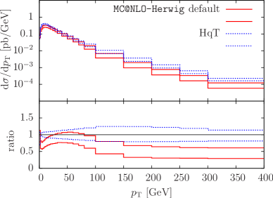
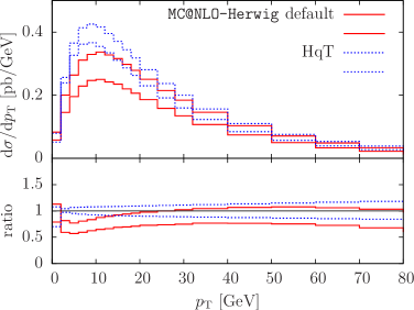
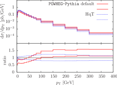
As shown earlier, a large difference in the high transverse momentum tail is visible. As can be seen immediately, when the uncertainty bands due to scale variations are included, the differences between the two NLO+PS methods, and their differences with respect to the HqT result, become less pronounced. The observation made earlier on the insensitivity of the shape of the $p_{\rm T}$ distribution contributed by $S$ (or ${\mathbb{S}}$) events is also visible, with the POWHEG shape being constant for all transverse momenta, and the MC@NLO shape being roughly constant in the region dominated by ${\mathbb{H}}$ events. It is also seen that the scale uncertainty in POWHEG corresponds to a uniform factor in the whole range of transverse momentum being considered.

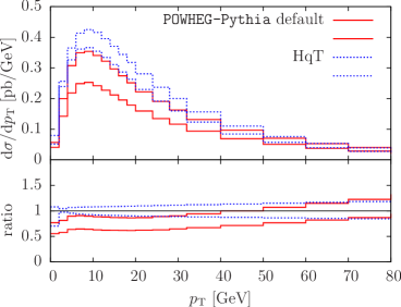
In order to give a more realistic assessment of the uncertainties in POWHEG, one can also exploit the freedom in the separation $R=R^{\rm S}+R^{\rm F}$. In the case of Higgs production, it is found that by choosing $h=M_{{}{{}{{{{{\mathrm{{{}{}{{H}}\mspace{-0.6mu}}}}}}}}}}/1.2$, the POWHEG result closely matches in shape that of HqT. It is similarly found that MC@NLO better matches the HqT output if $M_{{}{{}{{{{{\mathrm{{{}{}{{H}}\mspace{-0.6mu}}}}}}}}}}$, rather than $m_{\rm T}$, is used as central scale for scale variations. These results are shown in Figure 6.

Figure 6: Uncertainty bands for the transverse momentum spectrum of the Higgs boson at LHC, 7 TeV, for a higgs mass $m_{H}=120~{}\text{GeV}$. On the upper plots, the MC@NLO+HERWIG result obtained using the non-default value of the reference scale equal to $M_{{}{{}{{{{{\mathrm{{{}{}{{H}}\mspace{-0.6mu}}}}}}}}}}$. On the lower plots, the POWHEG+PYTHIA output, using the non-default $R^{\rm S}+R^{\rm F}$ separation. The uncertainty bands are obtained by changing $\mu_{\rm R}$ and $\mu_{\rm F}$ by a factor of two above and below the central value, taken equal to $M_{{}{{}{{{{{\mathrm{{{}{}{{H}}\mspace{-0.6mu}}}}}}}}}}$, with the restriction $0.5<\mu_{\rm R}/\mu_{\rm F}<2$.

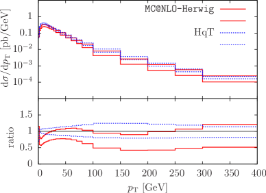
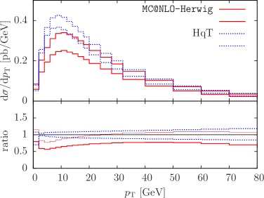
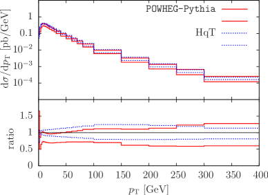
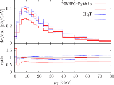
We see that now the large differences between MC@NLO and POWHEG are mostly removed, since both adopt a central scale equal to $M_{{}{{}{{{{{\mathrm{{{}{}{{H}}\mspace{-0.6mu}}}}}}}}}}$, and both adopt a similar separation of $S$ (or ${\mathbb{S}}$) and $F$ (or ${\mathbb{H}}$) events. Both generators, furthermore, display a reasonable scale variation in the high $p_{\rm T}$ regime, while the scale variation at moderate values of transverse momenta (around 100 GeV) seems to be comparable to that of HqT, rather than being larger.

In MC@NLO, we have seen that the shape of the transverse momentum spectrum at moderate $p_{\rm T}$ exhibits only a mild dependence upon scale variation. This shape is in fact determined by ${\mathbb{S}}$ events, and thus depends only upon the shower Monte Carlo that is being used, which is HERWIG in the present case. We may expect significant changes in shape if other Monte Carlos are used. In Figure 7 we display

Figure 7: Uncertainty bands for the transverse momentum spectrum of the Higgs boson at LHC, 7 TeV, for a higgs mass $m_{H}=120~{}\text{GeV}$. On the upper plots, the MC@NLO+PYTHIA result obtained using the non-default value of the reference scale equal to $M_{{}{{}{{{{{\mathrm{{{}{}{{H}}\mspace{-0.6mu}}}}}}}}}}$. The bare PYTHIA result rescaled by a $K$-factor is also shown.

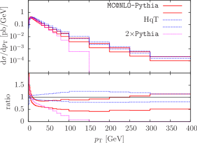
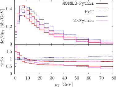
the Higgs $p_{\rm T}$ spectrum using MC@NLO with the virtuality-ordered version of PYTHIA [32]. We do indeed see a considerable difference in the spectrum at small transverse momenta. The discrepancy with HqT at small transverse momenta is purely due to the fact that the virtuality-ordered version of PYTHIA does not match well with HqT at small transverse momenta.

13 NLO+PS versus ME+PS matching

Matching tree-level matrix elements and parton shower generators (ME+PS) allows for the generation of samples where a basic process is accompanied by a fairly large number of associated jets. The ME+PS method was first formulated in ref. [1] (CKKW), and several variants have appeared since (for a summary of the various implementations see refs. [2, 71]). As a representative example, taking $W$ boson production as the basic process, the method allows one to construct a sample of $W$ with an arbitrary number of associated jets, where the distributions of the first $n$ jets ($n$ being limited by the computing power available) are computed with tree-level accuracy, and the remaining ones are generated in the collinear approximation. The ME+PS method does not achieve NLO accuracy for any quantity. However, it cannot be claimed that the NLO+PS methods are the NLO extension of the ME+PS method. In the example of $W$ production, an NLO+PS implementation of $W$ production can be used to produce a sample such that inclusive $W$ distributions, such as the $W$ rapidity distribution, are accurate at the NLO level. On the other hand, $W+1\,$jet production is described by this sample at order $\alpha_{\rm S}$, i.e. with the same level of accuracy as an ME+PS implementation. Furthermore, $W+2$ or more jets is generated in the NLO+PS only with shower accuracy, i.e. in the collinear approximation, while in the ME+PS sample it is generated with tree-level accuracy.

In ref. [64], the ALPGEN ME+PS generator was presented and a thorough comparison with MC@NLO was performed for top production. Figure 8 shows the

Figure 8: Comparison of MC@NLO and ALPGEN in top production, for a 14 TeV LHC, from ref. [64]. On the left, the transverse momentum of the top quark. On the right, the jet multiplicity.

main features of the comparison. Good agreement is found for inclusive quantities like the top quark transverse momentum distribution, provided that ALPGEN (which does not include NLO corrections) is rescaled by a $K$ factor. Once the $K$ factor is accounted for, the zero- and one-jet cross sections agree reasonably in the two approaches. At larger jet multiplicities we expect and see discrepancies between the two approaches, ALPGEN being more reliable in this case as it does not use the collinear approximation for the production of extra jets.

14 Outlook and further developments

The present NLO+PS implementations leave much room for improvement, and several papers in the literature propose new approaches. First of all, it would be desirable to merge the NLO+PS and ME+PS methods, in such a way that higher jet multiplicities are described at tree-level accuracy while inclusive observables maintain NLO accuracy. A further goal is the full extension of the ME+PS method to NLO, and several proposals in this direction have appeared in the literature [72, 73, 74, 75, 76]. Fixed-order NNLO calculations have become available for some collider processes, and their implementation in a shower framework would be welcome. Finally, a full extension of the shower algorithm to NLO, i.e. including NLO splitting kernels is being pursued [77, 78].

Besides pursuing new approaches, one can also investigate to what extent some of these objectives can be approached by simply merging event samples obtained with available tools. In ref. [79], a recipe for merging a POWHEG together with a MadGraph ME+PS sample is given for the cases of $W$ and $t\bar{t}$ production, and in ref. [80] a practical recipe is presented for merging the $Z$ and $Z+1$-jet POWHEG samples.

Appendix

Appendix A Smoothing procedure in MC@NLO

In this appendix we demonstrate that the smoothing procedure used in MC@NLO to cure an imperfect cancellation of soft divergences between $R$ and $R^{({\rm MC})}$ has only power-suppressed effects on infrared-safe observables. Although this is a technical point, we include it here just as an example of how the method used to prove NLO accuracy in Section 6 can also be applied to other important issues. First of all, in Section 10 we have shown that MC@NLO is equivalent to a POWHEG generator with $R^{\rm S}=R^{({\rm MC})}$, and thus the proof of NLO accuracy given in Section 6 can also be applied for MC@NLO.

Assume that the shower approximation for the real cross section is matched to the exact real cross section at a scale $Q_{m}$, i.e. that for transverse momentum of the radiation below $Q_{m}$, $R^{\operatorname{MC}}$ is smoothly matched to $R$. We write $R^{\operatorname{MC}}_{m}$ for the matched cross section. The proof of NLO accuracy in Section 6 goes more or less as before, and by the time we reach Equation 28, it has the following form

$$\sigma\langle O\rangle = \int d\Phi_{\mathrm{B}}\left[B+V+\int R^{\operatorname{MC}}_{m}\mathrm{d}\Phi_{\operatorname{rad}}\right]O(\Phi_{\mathrm{B}})+\int\mathrm{d}\Phi_{\mathrm{R}}R^{\operatorname{MC}}(O(\Phi_{R})-O(\Phi_{\mathrm{B}}))$$ (35)

$$+ \int\mathrm{d}\Phi_{\mathrm{R}}\left[R-R^{\operatorname{MC}}_{m}\right]O(\Phi_{R})$$

where we have assumed that $R^{\operatorname{MC}}_{m}$ replaces $R^{\operatorname{MC}}$ in the $\mathbb{S}$ events cross section $\overline{B}^{\operatorname{MC}}$, and in $R^{F}$, which is the cross section for $\mathbb{H}$ events. Each term in Equation 35 is finite, since $R^{\operatorname{MC}}_{m}$ matches $R$ in the singular region. We can easily manipulate Equation 35 as follows:

$$\sigma\langle O\rangle = \int d\Phi_{\mathrm{B}}\left[B+V+\int R\mathrm{d}\Phi_{\operatorname{rad}}\right]O(\Phi_{\mathrm{B}})+\int\mathrm{d}\Phi_{\mathrm{R}}R^{\operatorname{MC}}(O(\Phi_{R})-O(\Phi_{\mathrm{B}}))$$ (36)

$$+ \int\mathrm{d}\Phi_{\mathrm{R}}\left[R-R^{\operatorname{MC}}_{m}\right]\left[O(\Phi_{R})-O(\Phi_{\mathrm{B}})\right],$$

where, with respect to Equation 35, the term proportional to $O(\Phi_{\mathrm{B}})$ subtracted from the last term has been added to the first, and finally

$$\sigma\langle O\rangle = \int d\Phi_{\mathrm{B}}\left[B+V+\int R\mathrm{d}\Phi_{\operatorname{rad}}\right]O(\Phi_{\mathrm{B}})+\int\mathrm{d}\Phi_{\mathrm{R}}R(O(\Phi_{R})-O(\Phi_{\mathrm{B}}))$$ (37)

$$+ \int\mathrm{d}\Phi_{\mathrm{R}}\left[R^{\operatorname{MC}}-R^{\operatorname{MC}}_{m}\right]\left[O(\Phi_{R})-O(\Phi_{\mathrm{B}})\right].$$

The first line in Equation 37 corresponds to the exact NLO result, and the last line corresponds to the correction due to the smoothing procedure. Now we suppose that $\left[R^{\operatorname{MC}}-R^{\operatorname{MC}}_{m}\right]$ is singular in the singular region. However, $\left[O(\Phi_{R})-O(\Phi_{\mathrm{B}})\right]$ kills the singularity for infrared-safe observables, so, the integrand in Equation 37 is finite. Furthermore it vanishes if the transverse momentum of radiation is above $Q_{m}$, because $R^{\operatorname{MC}}=R$ in that case. Thus we have a power of $Q_{m}$ suppression, where the exact power depends upon how smoothly $O(\Phi_{R})$ approaches $O(\Phi)$ near the singular region.

References

- [1] S. Catani, F. Krauss, R. Kuhn, and B. Webber, QCD matrix elements + parton showers, JHEP 0111 (2001) 063, [hep-ph/0109231].
- [2] A. Buckley, J. Butterworth, S. Gieseke, D. Grellscheid, S. Hoche, et. al., General-purpose event generators for LHC physics, Physics Reports 504 (2011) 145–233, [1101.2599].
- [3] S. Frixione and B. R. Webber, Matching NLO QCD computations and parton shower simulations, JHEP 06 (2002) 029, [hep-ph/0204244].
- [4] P. Nason, A new method for combining NLO QCD with shower Monte Carlo algorithms, JHEP 11 (2004) 040, [hep-ph/0409146].
- [5] S. Frixione, P. Nason, and C. Oleari, Matching NLO QCD computations with Parton Shower simulations: the POWHEG method, JHEP 11 (2007) 070, [arXiv:0709.2092].
- [6] T. Kinoshita, Mass singularities of Feynman amplitudes, J.Math.Phys. 3 (1962) 650–677.
- [7] T. Lee and M. Nauenberg, Degenerate Systems and Mass Singularities, Phys.Rev. 133 (1964) B1549–B1562.
- [8] T. Sjöstrand, A Model for Initial State Parton Showers, Phys.Lett. B157 (1985) 321.
- [9] G. Gustafson and U. Pettersson, Dipole Formulation of QCD Cascades, Nucl.Phys. B306 (1988) 746.
- [10] M. Bengtsson and T. Sjöstrand, Coherent Parton Showers Versus Matrix Elements: Implications of PETRA - PEP Data, Phys.Lett. B185 (1987) 435.
- [11] S. Frixione, P. Nason, and B. R. Webber, Matching NLO QCD and parton showers in heavy flavour production, JHEP 08 (2003) 007, [hep-ph/0305252].
- [12] S. Frixione, E. Laenen, P. Motylinski, and B. R. Webber, Angular correlations of lepton pairs from vector boson and top quark decays in Monte Carlo simulations, JHEP 04 (2007) 081, [hep-ph/0702198].
- [13] S. Frixione, E. Laenen, P. Motylinski, and B. R. Webber, Single-top production in MC@NLO, JHEP 03 (2006) 092, [hep-ph/0512250].
- [14] S. Frixione, E. Laenen, P. Motylinski, B. R. Webber, and C. D. White, Single-top hadroproduction in association with a W boson, JHEP 07 (2008) 029, [arXiv:0805.3067].
- [15] C. Weydert et. al., Charged Higgs boson production in association with a top quark in MC@NLO, Eur. Phys. J. C67 (2010) 617–636, [arXiv:0912.3430].
- [16] S. Frixione, F. Stoeckli, P. Torrielli, B. R. Webber, and C. D. White, The MC@NLO 4.0 Event Generator, arXiv:1010.0819.
- [17] http://www.hep.phy.cam.ac.uk/theory/webber/MCatNLO/.
- [18] T. Toll and S. Frixione, Charm and bottom photoproduction at HERA with MC@NLO, Phys. Lett. B703 (2011) 452–461, [arXiv:1106.1614].
- [19] V. Hirschi et. al., Automation of one-loop QCD corrections, JHEP 05 (2011) 044, [arXiv:1103.0621].
- [20] G. Ossola, C. G. Papadopoulos, and R. Pittau, Reducing full one-loop amplitudes to scalar integrals at the integrand level, Nucl. Phys. B763 (2007) 147–169, [hep-ph/0609007].
- [21] G. Ossola, C. G. Papadopoulos, and R. Pittau, CutTools: a program implementing the OPP reduction method to compute one-loop amplitudes, JHEP 03 (2008) 042, [arXiv:0711.3596].
- [22] R. Frederix et. al., W and Z/gamma* boson production in association with a bottom-antibottom pair, JHEP 09 (2011) 061, [arXiv:1106.6019].
- [23] R. Frederix et. al., Four-lepton production at hadron colliders: aMC@NLO predictions with theoretical uncertainties, arXiv:1110.4738.
- [24] R. Frederix et. al., aMC@NLO predictions for Wjj production at the Tevatron, arXiv:1110.5502.
- [25] S. Hoeche, F. Krauss, M. Schonherr, and F. Siegert, A critical appraisal of NLO+PS matching methods, arXiv:1111.1220.
- [26] S. Hoeche, F. Krauss, M. Schonherr, and F. Siegert, W+n-jet predictions with MC@NLO in Sherpa, arXiv:1201.5882.
- [27] S. Frixione, F. Stoeckli, P. Torrielli, and B. R. Webber, NLO QCD corrections in Herwig++ with MC@NLO, JHEP 01 (2011) 053, [arXiv:1010.0568].
- [28] G. Corcella et. al., HERWIG 6.5: an event generator for Hadron Emission Reactions With Interfering Gluons (including supersymmetric processes), JHEP 01 (2001) 010, [hep-ph/0011363].
- [29] G. Corcella et. al., HERWIG 6.5 release note, hep-ph/0210213.
- [30] M. Bahr et. al., Herwig++ Physics and Manual, Eur. Phys. J. C58 (2008) 639–707, [arXiv:0803.0883].
- [31] S. Gieseke et. al., Herwig++ 2.5 Release Note, arXiv:1102.1672.
- [32] P. Torrielli and S. Frixione, Matching NLO QCD computations with PYTHIA using MC@NLO, JHEP 04 (2010) 110, [arXiv:1002.4293].
- [33] T. Sjostrand, S. Mrenna, and P. Z. Skands, PYTHIA 6.4 Physics and Manual, JHEP 05 (2006) 026, [hep-ph/0603175].
- [34] E. Boos, M. Dobbs, W. Giele, I. Hinchliffe, J. Huston, et. al., Generic user process interface for event generators, hep-ph/0109068.
- [35] P. Nason and G. Ridolfi, A positive-weight next-to-leading-order Monte Carlo for Z pair hadroproduction, JHEP 08 (2006) 077, [hep-ph/0606275].
- [36] S. Frixione, P. Nason, and G. Ridolfi, A Positive-Weight Next-to-Leading-Order Monte Carlo for Heavy Flavour Hadroproduction, JHEP 09 (2007) 126, [arXiv:0707.3088].
- [37] S. Alioli, P. Nason, C. Oleari, and E. Re, NLO vector-boson production matched with shower in POWHEG, JHEP 07 (2008) 060, [arXiv:0805.4802].
- [38] S. Alioli, P. Nason, C. Oleari, and E. Re, NLO Higgs boson production via gluon fusion matched with shower in POWHEG, JHEP 04 (2009) 002, [arXiv:0812.0578].
- [39] S. Alioli, P. Nason, C. Oleari, and E. Re, NLO single-top production matched with shower in POWHEG: s- and t-channel contributions, JHEP 09 (2009) 111, [arXiv:0907.4076]. [Erratum-ibid.1002:011,2010].
- [40] S. Alioli, P. Nason, C. Oleari, and E. Re, A general framework for implementing NLO calculations in shower Monte Carlo programs: the POWHEG BOX, JHEP 06 (2010) 043, [arXiv:1002.2581].
- [41] S. Alioli, P. Nason, C. Oleari, and E. Re, Vector boson plus one jet production in POWHEG, JHEP 01 (2011) 095, [arXiv:1009.5594].
- [42] P. Nason and C. Oleari, NLO Higgs boson production via vector-boson fusion matched with shower in POWHEG, JHEP 02 (2010) 037, [arXiv:0911.5299].
- [43] E. Re, Single-top Wt-channel production matched with parton showers using the POWHEG method, Eur. Phys. J. C71 (2011) 1547, [arXiv:1009.2450].
- [44] S. Alioli, K. Hamilton, P. Nason, C. Oleari, and E. Re, Jet pair production in POWHEG, JHEP 04 (2011) 081, [arXiv:1012.3380].
- [45] T. Melia, P. Nason, R. Rontsch, and G. Zanderighi, W+W-, WZ and ZZ production in the POWHEG BOX, JHEP 11 (2011) 078, [arXiv:1107.5051].
- [46] T. Melia, P. Nason, R. Rontsch, and G. Zanderighi, plus dijet production in the POWHEGBOX, Eur.Phys.J. C71 (2011) 1670, [arXiv:1102.4846].
- [47] C. Oleari and L. Reina, W +- b production in POWHEG, JHEP 1108 (2011) 061, [arXiv:1105.4488].
- [48] S. Alioli, S.-O. Moch, and P. Uwer, Hadronic top-quark pair-production with one jet and parton showering, arXiv:1110.5251.
- [49] E. Bagnaschi, G. Degrassi, P. Slavich, and A. Vicini, Higgs production via gluon fusion in the POWHEG approach in the SM and in the MSSM, arXiv:1111.2854.
- [50] M. Garzelli, A. Kardos, C. Papadopoulos, and Z. Trocsanyi, Z0 - boson production in association with a top anti-top pair at NLO accuracy with parton shower effects, arXiv:1111.1444.
- [51] A. Kardos, Z. Trocsanyi, and C. Papadopoulos, Top quark pair production in association with a Z-boson at NLO accuracy, arXiv:1111.0610.
- [52] M. Garzelli, A. Kardos, C. Papadopoulos, and Z. Trocsanyi, Standard Model Higgs boson production in association with a top anti-top pair at NLO with parton showering, Europhys.Lett. 96 (2011) 11001, [arXiv:1108.0387].
- [53] A. Kardos, C. Papadopoulos, and Z. Trocsanyi, Top quark pair production in association with a jet with NLO parton showering, Phys.Lett. B705 (2011) 76–81, [arXiv:1101.2672].
- [54] G. Bevilacqua, M. Czakon, M. Garzelli, A. van Hameren, A. Kardos, et. al., HELAC-NLO, arXiv:1110.1499.
- [55] T. Gleisberg, S. Hoeche, F. Krauss, M. Schonherr, S. Schumann, et. al., Event generation with SHERPA 1.1, JHEP 0902 (2009) 007, [arXiv:0811.4622].
- [56] L. D’Errico and P. Richardson, A Positive-Weight Next-to-Leading-Order Monte Carlo Simulation of Deep Inelastic Scattering and Higgs Boson Production via Vector Boson Fusion in Herwig++, arXiv:1106.2983.
- [57] L. D’Errico and P. Richardson, Next-to-Leading-Order Monte Carlo Simulation of Diphoton Production in Hadronic Collisions, arXiv:1106.3939.
- [58] K. Hamilton, A positive-weight next-to-leading order simulation of weak boson pair production, JHEP 01 (2011) 009, [arXiv:1009.5391].
- [59] K. Hamilton, P. Richardson, and J. Tully, A Positive-Weight Next-to-Leading Order Monte Carlo Simulation for Higgs Boson Production, JHEP 04 (2009) 116, [arXiv:0903.4345].
- [60] K. Hamilton, P. Richardson, and J. Tully, A Positive-Weight Next-to-Leading Order Monte Carlo Simulation of Drell-Yan Vector Boson Production, JHEP 10 (2008) 015, [arXiv:0806.0290].
- [61] S. Hoche, F. Krauss, M. Schonherr, and F. Siegert, Automating the POWHEG method in Sherpa, JHEP 04 (2011) 024, [arXiv:1008.5399].
- [62] K. Hamilton, P. Richardson, and J. Tully, A Modified CKKW matrix element merging approach to angular-ordered parton showers, JHEP 0911 (2009) 038, [arXiv:0905.3072].
- [63] S. Hoeche, F. Krauss, S. Schumann, and F. Siegert, QCD matrix elements and truncated showers, JHEP 0905 (2009) 053, [arXiv:0903.1219].
- [64] M. L. Mangano, M. Moretti, F. Piccinini, and M. Treccani, Matching matrix elements and shower evolution for top-quark production in hadronic collisions, JHEP 0701 (2007) 013, [hep-ph/0611129].
- [65] http://theory.fi.infn.it/grazzini/codes.html.
- [66] G. Bozzi, S. Catani, D. de Florian, and M. Grazzini, The q(T) spectrum of the Higgs boson at the LHC in QCD perturbation theory, Phys.Lett. B564 (2003) 65–72, [hep-ph/0302104].
- [67] G. Bozzi, S. Catani, D. de Florian, and M. Grazzini, Transverse-momentum resummation and the spectrum of the Higgs boson at the LHC, Nucl.Phys. B737 (2006) 73–120, [hep-ph/0508068].
- [68] D. de Florian, G. Ferrera, M. Grazzini, and D. Tommasini, Transverse-momentum resummation: Higgs boson production at the Tevatron and the LHC, JHEP 1111 (2011) 064, [arXiv:1109.2109].
- [69] LHC Higgs Cross Section Working Group Collaboration, S. Dittmaier et. al., Handbook of LHC Higgs Cross Sections: 2. Differential Distributions, arXiv:1201.3084. 275 pages, 136 figures, to be submitted to CERN Report. Working Group web page: https://twiki.cern.ch/twiki/bin/view/LHCPhysics/CrossSections.
- [70] A. D. Martin, W. J. Stirling, R. S. Thorne, and G. Watt, Parton distributions for the LHC, Eur. Phys. J. C63 (2009) 189–285, [arXiv:0901.0002].
- [71] J. Alwall et. al., Comparative study of various algorithms for the merging of parton showers and matrix elements in hadronic collisions, Eur. Phys. J. C53 (2008) 473–500, [arXiv:0706.2569].
- [72] Z. Nagy and D. E. Soper, Matching parton showers to NLO computations, JHEP 0510 (2005) 024, [hep-ph/0503053].
- [73] W. T. Giele, D. A. Kosower, and P. Z. Skands, A Simple shower and matching algorithm, Phys.Rev. D78 (2008) 014026, [arXiv:0707.3652].
- [74] N. Lavesson and L. Lonnblad, Extending CKKW-merging to One-Loop Matrix Elements, JHEP 0812 (2008) 070, [arXiv:0811.2912].
- [75] C. W. Bauer, F. J. Tackmann, and J. Thaler, GenEvA. I. A New framework for event generation, JHEP 0812 (2008) 010, [arXiv:0801.4026].
- [76] C. W. Bauer, F. J. Tackmann, and J. Thaler, GenEvA. II. A Phase space generator from a reweighted parton shower, JHEP 0812 (2008) 011, [arXiv:0801.4028].
- [77] M. Skrzypek, S. Jadach, A. Kusina, W. Placzek, M. Slawinska, et. al., Fully NLO Parton Shower in QCD, Acta Phys.Polon. B42 (2011) 2433–2443, [arXiv:1111.5368].
- [78] S. Jadach, A. Kusina, W. Placzek, M. Skrzypek, and M. Slawinska, On the inclusion of the QCD NLO corrections in the quark–gluon Monte Carlo shower, arXiv:1103.5015.
- [79] K. Hamilton and P. Nason, Improving NLO-parton shower matched simulations with higher order matrix elements, JHEP 1006 (2010) 039, [arXiv:1004.1764].
- [80] S. Alioli, K. Hamilton, and E. Re, Practical improvements and merging of POWHEG simulations for vector boson production, arXiv:1108.0909.