Individual Eigenvalue Distributions for the Wilson Dirac Operator
Abstract
We derive the distributions of individual eigenvalues for the Hermitian Wilson Dirac Operator as well as for real eigenvalues of the Wilson Dirac Operator . The framework we provide is valid in the epsilon regime of chiral perturbation theory for any number of flavours and for non-zero low energy constants . It is given as a perturbative expansion in terms of the -point spectral density correlation functions and integrals thereof, which in some cases reduces to a Fredholm Pfaffian. For the real eigenvalues of at fixed chirality this expansion truncates after at most terms for small lattice spacing . Explicit examples for the distribution of the first and second eigenvalue are given in the microscopic domain as a truncated expansion of the Fredholm Pfaffian for quenched , where all -point densities are explicitly known from random matrix theory. For the real eigenvalues of quenched at small we illustrate our method by the finite expansion of the corresponding Fredholm determinant of size .
1 Introduction
At low energies Quantum Chromodynamics (QCD) has a very convenient analytical testing ground, the so-called epsilon regime of chiral perturbation theory (XPT) [1]. In this limit standard XPT is reduced to a group integral over the zero-momentum modes that are then non-perturbative and dominate the theory, times a Gaussian free field theory of propagating Goldstone bosons. Although being an unphysical limit the analytic predictions in this regime are useful and can be tested against numerical results from lattice gauge theory. Of particular interest for the establishment of chiral symmetry breaking and the effect of gauge field topology is the Dirac operator spectrum. There are several equivalent methods to compute correlation functions of Dirac operator eigenvalues in this regime. Either one starts from XPT in a partially quenched also called graded setting which is based on supergroup integrals, see e.g. [2], or equivalently one can use replicated partition functions [3]. Yet another method that was actually first proposed in [4] uses chiral Random Matrix Theory (RMT), being equivalent to the epsilon regime of XPT at leading order (LO) [2, 5]. This latter approach is best suited to compute the distribution of individual Dirac operator eigenvalues [6, 7] - which in turn are particularly clean objects for a comparison with lattice data.
In the continuum limit this setup has already been very useful, in order to determine the low energy constants (LEC) in the chiral Lagrangian or to test lattice algorithms for their topology dependence, and we refer to [8] for a recent review including references. In XPT there are only two LEC to LO, the chiral condensate which is the order parameter of chiral symmetry breaking, and the Pion decay constant . Individual Dirac operator eigenvalues allow for a very detailed error analysis in the determination of compared to the average density through the Banks-Casher relation, and we refer e.g. to [9] for recent work. In order to make the epsilon regime also sensitive to a coupling to imaginary iso-spin chemical potential has been proposed and realised in [10]. This leads to realistic values of when computing and optimising higher order corrections [11]. The computations were done in a partially quenched setting, where a -dependent Dirac operator is probed with -independent configurations. A wealth of results exists for the density correlation functions with [10, 12, 11] and without [4, 13], as well as for individual eigenvalue distributions with [14, 15] and without [6, 7].
What happens if one wants to include the effect of finite lattice spacing , which is unavoidably present in all simulations? Perhaps surprisingly the effect is much simpler in Wilson XPT developed in [16, 17], than in its staggered version [18]. This is despite the fact that the Wilson term completely breaks chiral symmetry whereas the staggered Dirac operator partly preserves it. In a Symanzik type expansion Wilson XPT requires three extra LEC to LO, that have to be determined in order to quantify the effect of a finite lattice spacing111This is so even though they represent unphysical lattice artefacts, with their values depending on the lattice action considered., and we refer to [19] for review articles.
The epsilon regime with Wilson fermions was put into focus in [20], addressing mesonic correlation functions. Then two years ago the microscopic spectral density of the Wilson Dirac operator in the epsilon regime was computed [21]. The study of this operator has since seen a remarkably fast progress. First of all one has to distinguish between the non-Hermitian Wilson Dirac operator and its Hermitian version , and their corresponding densities. While we refer to ref. [22] for a discussion of the relation between topology and chirality at finite-, and to ref. [23] for the distinction of left and right eigenvalues for , let us give a short list of what is known to date about the eigenvalue correlation functions.
The quenched microscopic density for and for the real eigenvalues of were computed in [21, 22], respectively. These results were extended to flavours in [24, 25] and to in [26]. There, also the quenched two-point eigenvalue density was given explicitly, and a computational scheme for higher densities and was set up although it rapidly becomes cumbersome. In [27] all quenched higher density correlations were computed for at . The corresponding results for the complex density of eigenvalues including all were given in [23], where further results to all orders were announced which have just appeared [28]. Most of the previous results for the density (except [25]) were given for and , which is expected to be a good approximation for a large number of colours [29]. However, it was also understood in [22] how to derive results from results on the level of XPT by one extra Gaussian integration per LEC. This was now extended to an RMT setting in [28]. Furthermore, in [22] it was shown that in the epsilon regime QCD inequalities lead to a restriction on the sign of to be positive for . This constraint was very recently extended to different combinations of LEC [30, 31, 32]. We note that the signs (of combinations) of these LEC are not merely of academic interest, but decide crucially on the scenarios of possible phase transitions, see e.g. the discussion in [17, 30, 32]. Finally we would also like to mention the computation of the mean spectral density of in [33].
Based on previous experience at how useful individual eigenvalue distributions are, in [34, 35] first lattice simulations to compare to the above epsilon regime predictions at were made. There the individual eigenvalue distributions were generated numerically from RMT. We fill this gap here by providing the framework of how to analytically compute these distributions. This setup holds for general and non vanishing LEC . Our explicit examples are all quenched and at , but our framework can be used for all higher density correlations for and at that are available.
The content of this paper is organised as follows. In section 2 we set up the general framework of how to compute individual eigenvalue distributions or their cumulative distributions in terms of density correlation functions which we assume to be given. In section 3 we then specify the joint probability distributions for - (subsect. 3.1) and real -eigenvalues (subsect. 3.2) based on RMT. At this leads to a closed Fredholm Pfaffian expression for the former, and a distribution of finitely many real eigenvalues at small spacing for the latter. Section 4 is devoted to explicit examples in the microscopic or epsilon regime. For quenched we give the first and second eigenvalue in a truncated expansion of the Fredholm Pfaffian (subsect. 4.1). In the case of (subsect. 4.2) the approximate distributions are given in a finite series of expansion terms for . Our conclusions are summarised in section 5.
2 Individual eigenvalue distributions: general theory
In this section we describe the general formalism how to compute the distribution of individual eigenvalues and their cumulative distribution, having the Wilson Dirac operator and its Hermitian counterpart in mind. We will focus on real eigenvalues here, although this setup can also be generalised to complex eigenvalues after choosing a family of contours to order them, and we refer to [36] for details in the case of a real chemical potential.
Our starting point is chosen to be quite broad, given in terms of a partition function and its joint probability distribution (jpdf) of all eigenvalues that is invariant under permutations of eigenvalues, without further symmetry requirements. In particular we do not require the jpdf to be a determinant or Pfaffian in this section. As an example the jpdf can be obtained from the corresponding random two-matrix models and their representation in terms of - or real -eigenvalues, which we will specify in section 3. Note that when introducing by extra Gaussian integrations [22, 32, 28] the resulting jpdf is no longer a determinant or Pfaffian. Therefore it is important to be more general here. Our final expressions for individual eigenvalues will only contain -point spectral densities and their integrals. For that reason this setup also applies to partially quenched XPT where these densities can be generated by introducing pairs of fermionic and bosonic source terms. The analogous statement for spacing was reported in [37].
We begin by defining the partition function of the theory under consideration,
| (2.1) |
It is given by real integrals over the so-called joint probability distribution function , which is taken to be invariant under permutations of all eigenvalues, without further symmetry requirement. It may depend on external parameters such as quark masses, the number of flavours or the chirality. We also define the -point density correlation function,
| (2.2) |
normalised by the partition function. The simplest example is just the spectral density for . For the density is simply the normalised jpdf itself, . The are supposed to be known in the following as all other quantities will be expressed in terms of them.
The -th gap probability or cumulative distribution is defined as follows:
| (2.3) |
for . It is proportional to the probability of having exactly out of eigenvalues inside the interval , and eigenvalues outside this interval. Note that we do not specify any ordering among the or eigenvalues respectively, nor do we specify how many of the eigenvalues are less than or larger than (we assume without loss of generality). The simplest example with gives the probability of having empty of eigenvalues.
A remark is in order here. In the simplest jpdf we have in mind here that describes the transition from the Gaussian Unitary Ensemble (GUE) to the chiral GUE in RMT, the eigenvalues live on the full real line and cannot be restricted to the positive half line . In particular there is no chiral symmetry as for the chiral GUE, that for every eigenvalue there is also an eigenvalue at . Only on average the distributions of individual eigenvalues may be symmetric with respect to the origin in some special case (). Apart from that the derivation here is only a mild generalisation of [37] which we follow closely. Note also that we will still count the eigenvalues from the origin onwards, e.g. by choosing for the positive eigenvalues, as this is where the microscopic large- limit will be taken eventually.
Rewriting , applying the binomial formula and using the permutation invariance of the jpdf we can rewrite the -th gap probability as
| (2.4) | |||||
where for the first term in the last sum is unity. For the simplest example we thus have
| (2.5) | |||||
where we only show the first few terms in the sum containing terms. Note however that when considering the number of real eigenvalues of , we can set to a good approximation at small , and then we will only need a small and fixed number of terms. In particular for eq. (2.5) would be exact, and for we only have the first 3 terms222For with a single eigenvalue no new information is gained from compared to the density itself, see also eq. (2.12) for the first eigenvalue.. For the Hermitian Wilson Dirac operator , will become proportional to the number of eigenvalues and thus will be taken to infinity. Even in that case taking only the first few terms in the now infinite series eq. (2.4) will yield an excellent approximation, as we will see in section 4 and as was known already for [37].
The -th gap probability can be most conveniently written in terms of a generating function,
| (2.6) |
We then have
| (2.7) |
The probability of having one eigenvalue at the upper boundary , with eigenvalues in and all other eigenvalues outside this interval is defined as
| (2.8) | |||||
for . For example if we choose and this gives the distribution of the first positive eigenvalue on . The can be obtained by differentiation from the corresponding gap probability as we will show below. Analogously we can define the probability of having one eigenvalue at the lower boundary , with eigenvalues in and all other eigenvalues outside this interval:
| (2.9) | |||||
for . This definition is convenient when counting negative eigenvalues from the origin onwards. For example the first negative eigenvalue on follows by differentiating with respect to and by choosing .
The explicit relation between individual eigenvalue distributions and gap probabilities are as follows, where we restrict ourselves to the . The relations for the are similar. We obtain from by differentiation
| (2.10) |
(with ) or, after taking the sum on both sides,
| (2.11) |
In the case of the simplest example and the expansion eq. (2.5) maps to
| (2.12) |
for the distribution of the first positive eigenvalue on after choosing , and
| (2.13) |
for the second positive eigenvalue. Note again that if we had here, the expressions in eqs. (2.12) and (2.13) would be exact, without further corrections.
3 Application to the Wilson Dirac operators and
In this section we specify to the two RMT for the Wilson Dirac operator and its Hermitian counterpart for an arbitrary number of flavours , and give their respective jpdf. In the limit of large matrices specified in the next section 4 they describe the epsilon regime of Wilson XPT.
3.1 The jpdf and quenched -point densities of
We begin with the RMT for the Hermitian Wilson Dirac operator with in the form as it was introduced in [27], apart from putting an explicit -dependence into the weight function here. The partition function is defined as
| (3.1) | |||||
| (3.4) |
where we have introduced the Hermitian random matrix333Note that in the original proposal [22] instead of a full matrix only two Hermitian matrices were added on the diagonal blocks, similar to eq. (3.22). of size with and the complex random matrix of size . Here will be kept fixed and of order one, it plays the rôle of chirality [22]. The parameter incorporates the influence of the lattice spacing times the LEC, , see eq. (4.2) for the precise mapping between RMT and XPT quantities. It also allows to interpolate between the chiral GUE () and the GUE () in RMT when setting . The real parameters and denote the standard quark mass and sources for , respectively. The jpdf for the eigenvalues of was derived in [27] to where we refer for details, and we only give the result valid up to an overall (-dependent) constant:
| (3.7) | |||||
| (3.8) |
Here denotes the standard Vandermonde determinant. We have also defined the antisymmetric weight function
| (3.9) | |||||
appearing inside the Pfaffian. It could also be written in terms of the generalised incomplete error function (c.f. [23]). Note that the Jacobian from the diagonalisation of is not a simple Vandermonde determinant to some integer power, as it is in standard one-matrix models. The additional Pfaffian determinant containing part of the weight function is a feature shared by the partition function for the non-Hermitian Wilson Dirac operator eq. (3.19) [23], as well as by other non-Hermitian RMT, see [38].
The problem of computing individual eigenvalue distributions in terms of densities is now specified. All -point density correlation functions have been computed explicitly in the quenched approximation for [27]. For higher for and the spectral density has been computed explicitly in [22, 24, 25, 26], respectively. There, the supersymmetric or graded eigenvalue method was used starting from the partially quenched chiral Lagrangian, but the results agree because of universality. Unfortunately from the density alone being the first term in eq. (2.12) we do not gain any new information regarding the first eigenvalue. Let us emphasise that this lack of present information is not a restriction of our method. With the more general results for all -point density correlation functions for arbitrary and now at hand [28], these can be simply inserted into our setup without modifications.
We continue to recall some of the results of [27]. For and all -point density correlation functions can be written as the Pfaffian of a matrix valued kernel ,
| (3.10) |
For finite- and its matrix elements read (we refer to [27] for details, including ):
| (3.11) |
with the corresponding skew-orthogonal polynomials and their integral transforms being given by
| (3.12) | |||||
| (3.13) |
In particular the jpdf, eq. (3.10) for , can be written as a single Pfaffian for both :
| (3.14) |
which extends to [28]. Inserting eq. (3.10) into the generating function for all gap probabilities eq. (2.6) it becomes a Fredholm Pfaffian [39] and can thus be written in a closed form
| (3.15) | |||||
Here the are the eigenvalues of the matrix integral equation . We will come back to the perturbative evaluation of this Fredholm Pfaffian after taking the microscopic large- limit in section 4.
Finally we would like to discuss the inclusion of , following [22]. There, it was first understood how to include these terms on the level of the XPT partition function, by introducing two extra Gaussian integrations and shifting the source terms for masses and , respectively. While the RMT partition function matches this only in the microscopic limit444The quenched partition function has to be - and -independent for that, unlike the convention in [27]., it is tempting to assume that an RMT for can be constructed at finite-, which was recently achieved in [28]. The integral transformed jpdf is non-trivial in general, and special care has to be taken regarding the normalisation when computing spectral densities and individual eigenvalue distributions of such RMT (see e.g. [40] for a similar discussion).
In particular it leads not only to a shift of the masses, but partly of the eigenvalues which can be viewed as extra auxiliary masses in the graded framework [22] (c.f. [32, 28]). If we define an RMT jpdf including [32]
| (3.16) |
and a corresponding RMT partition function we obtain for the -point density
| (3.17) | |||||
where we explicitly display all arguments here. We have checked that the resulting microscopic density agrees with that following from the resolvent in [22] in various cases. Because eq. (2.4) is a liner map this translates as follows to individual eigenvalues,
| (3.18) | |||||
making our framework directly applicable in this setting too.
3.2 The jpdf of
We now turn to the RMT for the non-Hermitian Wilson Dirac operator following [22], first at :
| (3.19) | |||||
| (3.22) |
The Hermitian random matrices and are of sizes and , respectively. Here the parameter is not restricted and the masses can in principle be taken non-degenerate. The Dirac matrix can only be quasi-diagonalised and we refer to [23] for details where the jpdf was computed. Choosing without loss of generality, the eigenvalues of consist of complex conjugate eigenvalue pairs, of real right eigenvalues and of real left eigenvalues. Here can take any value , and we have to sum over all possible sectors. The partition function can thus be written as follows [23] for :
| (3.27) | |||||
Here we defined two different jpdf, with a fixed number of real right eigenvalues , and without fixing . We note in passing that the latter jpdf in eq. (3.27) can also be written in terms of a single Pfaffian [28]. The one- and two-dimensional delta-functions in the variables inside the determinant assure that we sum over all possible sectors. This sum is explicitly given in the last equation. The respective weight functions are defined as [23]
| (3.28) | |||||
| (3.29) | |||||
| (3.30) |
The fact that we have to distinguish between left and right eigenvalues of leads to more possibilities of defining density correlation functions, compared to eq. (2.2). When defining the density by inserting a delta-function into the jpdf we encounter a density of complex, of left and of right real eigenvalues, respectively. For example following [23] the density of complex eigenvalues, , and the density of real right eigenvalues is defined as
| (3.31) |
and likewise for the density of real left eigenvalues . It is clear by comparing to eq. (3.27) that in principle both densities get contributions from all sectors . Note that in [23] a particular combination of these densities was defined, the so-called density of chirality:
| (3.32) |
Higher -point correlation functions have to be split as well. For example the 2-point function will have 3 contributions: to find 2 complex eigenvalues, one complex and one real, and two real eigenvalues; and so on for higher .
We would like to point out that if one is only interested in the correlation functions of real eigenvalues as we are here, at least approximately one can obtain the situation of having a jpdf of only finitely many real left eigenvalues in the large- limit. Hence for this setting expanding the Fredholm determinant to obtain the first individual eigenvalue truncates at exactly terms. In [23] the probability to obtain more real (right and left) eigenvalues in addition to was computed as a function of the rescaled spacing and of , see figure 4 in [23]. For example for a value of there are less than additional real eigenvalues for (and even less for ), that is contributions from sectors with . Restricting ourselves to the sector we can thus define an approximate jpdf for the real eigenvalues valid for small :
| (3.33) |
We can now follow eqs. (2.2) and (2.4) with there, and we only need to insert the -point densities of real left eigenvalues for up to , with being small and finite. Note that in this approximation we have that
| (3.34) |
This is consistent when comparing to figures 5 and 6 in ref [23] for small values of .
4 Examples for individual real eigenvalues in the microscopic limit
In this section we will give explicit examples for individual eigenvalue distributions. Because RMT is only equivalent to Wilson XPT in the epsilon regime after taking the microscopic large- limit, we directly give results in this limit and refer to the literature for details. We present only quenched higher -point density correlation functions as an example, which we need in our expansion. However, as it should have become clear from the previous sections our method is not restricted to this case, it could immediately be applied to unquenched densities too. As a further simplification we choose to work here with . Again this restriction is not a principle one, and we have shown how to lift it following [22]. To keep everything as simple and transparent as possible we choose to work with only.
The examples for the quenched Hermitian Wilson Dirac operator are presented in subsection 4.1, and the examples for the distribution of real eigenvalues of the Wilson Dirac operator follow in subsection 4.2.
4.1 Hermitian Wilson Dirac operator
The computation of the microscopic large- limit was discussed in great detail in ref. [27] which we shall not repeat here, recalling only the results. The only difference to ref. [27] here is the extra factor of in the exponent of the weight function in eq. (3.1). We have chosen this convention here, to be achieved by a simple rescaling of all matrix elements, in order to have the same microscopic rescaling of the eigenvalues , masses and lattice spacing as for in the conventions of ref. [23].
The microscopic quantities denoted by hat are defined as follows:
| (4.1) |
The map to the LEC in the chiral Lagrangian is provided by
| (4.2) |
where is the volume, the chiral condensate, the lattice spacing and the LEC. The microscopic -point density correlation functions have to be rescaled appropriately with ,
| (4.3) |
with all the arguments on the right hand side rescaled according to eq. (4.1). The rescaled microscopic gap probabilities are defined as
| (4.4) |
and correspondingly the resulting rescaled individual eigenvalue distributions and follow. Hence the boundaries of the interval considered have to be rescaled in the same way as the eigenvalues in eq. (4.1).
We will now give the building blocks of the limiting microscopic kernel. All 3 kernels in eq. (3.11) can be expressed through the kernel , the weight function eq. (3.9) and integrals thereof, plus some extra terms for . Referring to [27] for details we have for our first example at :
| (4.5) | |||||
| (4.6) | |||||
| (4.7) |
where
| (4.8) |
is the rescaled, microscopic weight eq. (3.9). One of the integrals can be computed analytically,
| (4.9) |
However, this is not always advantageous when plotting the densities. From these building blocks we obtain the following expressions for the densities:
| (4.10) |
and for general
| (4.11) |

As our first example we will now give the distribution of the first, second and third positive eigenvalue of for , using only the first 3 densities with as an approximation when truncating the Fredholm Pfaffian expansion. In order to describe the first positive eigenvalue from the origin we choose as the interval for the gap probability, differentiate with respect to the upper bound and rescale . Using eq. (2.11) at this level of truncation we obtain on
| (4.12) | |||||
| (4.13) | |||||
| (4.14) |
Their generating cumulative distributions are obvious. Note that when summing up these first 3 approximate individual eigenvalue distributions eqs. (4.12) - (4.14) we trivially get the exact density. Would we add the exact individual eigenvalue distributions instead, this identity would only hold after summing up all eigenvalues, .
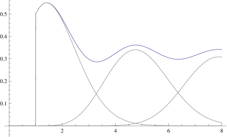
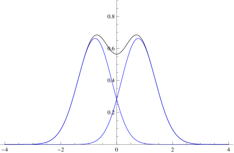
Inserting the above expressions eqs. (4.10) and (4.11) together with eqs. (4.5)-(4.8) leads to the curves shown in figure 1 (top plot). From it we see that our approximation gives well localised curves for the 1st and 2nd eigenvalue. While the 1st eigenvalue smoothly touches zero at around , clearly the approximation gets worse for the 2nd and even more so for the 3rd eigenvalue. To get a similar quality for the 2nd eigenvalue we would need to include up to terms containing , and for the 3rd eigenvalue terms up to . The fact that the left tail of the first positive eigenvalue is not shown for this value of is an artefact of counting eigenvalues from the origin. If we were to use another interval (say ) we could also determine this tail. However, the origin is a good point to choose since in the limit chiral symmetry is restored.
It is clearly seen when the approximation breaks down at latest: that is when increases again from zero for large , when becomes negative for the second eigenvalue, and when exceeds the spectral density which is an upper bound to all individual eigenvalue distributions. This breakdown happens roughly at the same point , up to which we can trust our approximated individual distributions (see also fig. 3 left). This is because from this point onwards the 4th eigenvalue would start contributing which is zero to our order of approximation. Nevertheless even the first part of the ascending curve of the 3rd eigenvalue could be used for fitting purposes to this order. In order to illustrate the described convergence of our approximation scheme we show in fig. 2 the same plot as fig. 1 (top plot), using one term less in the approximation: the density and the two-point function.
 ,
,
Let us also compare our approximate distributions in fig. 1 (top plot) with the corresponding first, second and third eigenvalues when the lattice spacing , as shown in fig. 1 (bottom plot). In this limit also the individual eigenvalue distributions and microscopic density are known exactly:
| (4.15) | |||||
| (4.16) | |||||
| (4.17) |
Here we only give the first eigenvalue distributions following [6]. The expressions for higher eigenvalues can be found in [7]. In order to compare to the eigenvalues which contain the mass, cf. eq. (3.4), we need to shift the density eq. (4.17) as in [22],
| (4.18) |
and the individual eigenvalue distributions accordingly. These shifted distributions are plotted in fig. 1 (bottom plot). It can be clearly seen that the first eigenvalue is most sensitive to the influence of , for which we have the best approximation.
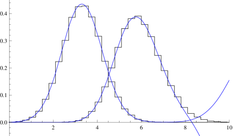
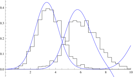
We would like to compare our new analytical predictions for individual eigenvalues with RMT and lattice data, following very recent comparisons [34, 35] where numerically generated curves for RMT were used. As an illustration we use the RMT and lattice data from fig. 8 in ref. [34], shown in our figure 3 left and right, respectively. Our approximate analytical curves for the individual eigenvalues match very well the numerically generated RMT histograms from [34] in the left plot as they should. In the comparison to the lattice data - these are predictions from other data in [34] and not fits to these curves - one can see a slight systematic shift to the left. Our analytic curves clearly are a very sensitive tool to fit lattice data. Compared to fits of the spectral density also used in [34, 35], individual eigenvalues have an unambiguous normalisation to unity.

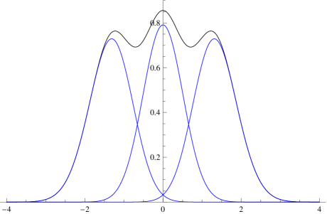
Let us now turn to our second example at . Here the building blocks for the kernel read [27]:
| (4.19) | |||||
| (4.21) | |||||
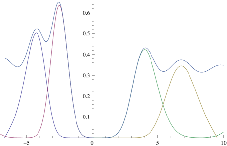
We simply have to insert these into eq. (4.11) to obtain the densities, and into eqs. (4.12) - (4.14) to obtain the individual eigenvalues to our order of approximation. The corresponding curves are shown in figure 4 (top plot). Note that the spectral density is no longer symmetric with respect to the origin. This is due to the broadening by of the single zero eigenvalue () which is shifted to the location of the mass, . The first and second negative eigenvalue is determined separately using the quantities eq. (2.9), that is by differentiating the gap probability with respect to the lower bound of the gap . When comparing to the same curves at in figure 4 (bottom plot), the first (“non-zero”) negative eigenvalue there becomes the second negative eigenvalue for in the top plot, and receives considerable corrections as well.
4.2 Real eigenvalues of the Wilson Dirac operator
For -point correlation functions of left (or right) real eigenvalues of much less was known compared to the previous subsection for . Explicit results included only the quenched and -point function for arbitrary . More general results for all quenched -point functions have been announced [23] and appeared now [28]. For it is either given as the discontinuity of the corresponding resolvent [22], or more explicitly as a double integral in [23]. For its resolvent is given as a 4-fold integral over a determinant times some rational function [26]. As expected this result can be factorised and brought into a Pfaffian form [28], in analogy to [41]. Plotting the integral in the form of [26] would still be a formidable task. It would give us a good approximation to the first real eigenvalue and to the ascent of the second one.
Rather than awaiting more tractable results announced in [23] that have appeared after finishing this paper [28], let us illustrate our method in the small -regime. Here it was shown [22] that the microscopic limit of the spectral density becomes a GUE distribution (just as the broadening of the zero-modes of ). We therefore expect that the jpdf will be given by that of the GUE for matrices. This is based on the analogy to , where the factorisation of the jpdf into a GUE part for the broadened zero-modes and a chiral GUE part for the remaining eigenvalues was shown in [27]. We thus can write approximately for and
| (4.22) |
where the GUE kernel inside the determinant is given by
| (4.23) |
In this regime all microscopic eigenvalues are measured in units of . The spectral density
| (4.24) |
is then simply the Wigner semi-circle for finite . Higher -point density correlation functions follow easily from eq. (4.22),
| (4.25) |
for . Based on these expressions, we can now give all individual eigenvalue distributions by a finite number of terms for the gap probability. In this case it is a Fredholm determinant of size , which after expansion gives rise to terms.
In figure 5 we show the spectral density and the individual eigenvalues for . As the gap interval we have to chose here . For for example the distribution of the first and second eigenvalues given in eqs. (2.12) and (2.13) are exact, without the dots. For we can use eqs. (4.12) - (4.14) for the first three eigenvalues which are now exact, and so on for higher .
We mention in passing that for a jpdf with such a small and fixed number of eigenvalues there exists an alternative computation instead of the Fredholm determinant. The individual eigenvalue distributions could also be computed as integrals over the ordered set of eigenvalues,
| (4.26) | |||||
| (4.27) |
etc., and then normalising them appropriately.
5 Conclusions
We have set up a framework to analytically compute the distribution of individual real eigenvalues, both for the Wilson Dirac operator and its Hermitian counterpart in the epsilon regime of Wilson chiral perturbation theory. These distributions are given in a perturbative expansion of -point density correlation functions and integrals thereof. For small lattice spacing and for the real eigenvalues this expansion truncates after terms where plays the rôle of chirality on the lattice. As an example for quenched all -point density correlation functions are presented for and we have given the resulting distributions of the first two positive and two negative eigenvalues as a function of the low energy constant times the lattice spacing squared as an illustration. Our results very well describe previous numerical results in the literature to the given order. We have briefly discussed how to include the effects of in our framework. Hopefully this setup will become useful in the precise determination of all low energy constants to leading order. This is especially so because more analytic density correlation functions have just become available after finishing this paper [28].
It would be very interesting to try to understand the mismatch discussed in [34] between lattice data and the analytical distribution of a single real eigenvalue of (which is equal to the density as in that case ). However, considering possible higher order effects in chiral perturbation theory is beyond the scope of this article.
Acknowledgements: The participants of the workshop “Chiral dynamics with Wilson fermions” at ECT* Trento in October 2011 are thanked for inspiring talks and discussions. We would also like to thank the authors of [34] for making some of their numerical lattice and RMT data available to us. We are indebted to Mario Kieburg, Kim Splittorff and Jac Verbaarschot for comments and discussions on the first version of this manuscript.
References
- [1] J. Gasser and H. Leutwyler, Phys. Lett. B 184 (1987) 83.
- [2] P. H. Damgaard, J. C. Osborn, D. Toublan and J. J. M. Verbaarschot, Nucl. Phys. B 547 (1999) 305 [hep-th/9811212].
- [3] P. H. Damgaard and K. Splittorff, Phys. Rev. D 62 (2000) 054509 [hep-lat/0003017].
- [4] E. V. Shuryak and J. J. M. Verbaarschot, Nucl. Phys. A 560 (1993) 306 [hep-th/9212088].
- [5] D. Toublan and J. J. M. Verbaarschot, Nucl. Phys. B 603 (2001) 343 [hep-th/0012144]; F. Basile and G. Akemann, JHEP 0712 (2007) 043 [arXiv:0710.0376 [hep-th]].
- [6] S. M. Nishigaki, P. H. Damgaard and T. Wettig, Phys. Rev. D 58 (1998) 087704 [hep-th/9803007].
- [7] P. H. Damgaard and S. M. Nishigaki, Phys. Rev. D 63 (2001) 045012 [hep-th/0006111].
- [8] P. H. Damgaard, “Chiral Random Matrix Theory and Chiral Perturbation Theory”, Lectures at the XIV Mexican School on Particles and Fields 2010, arXiv:1102.1295 [hep-ph].
- [9] F. Bernardoni, P. Hernandez, N. Garron, S. Necco and C. Pena, Phys. Rev. D 83 (2011) 054503 [arXiv:1008.1870 [hep-lat]].
- [10] P. H. Damgaard, U. M. Heller, K. Splittorff and B. Svetitsky, Phys. Rev. D 72 (2005) 091501 [hep-lat/0508029]; P. H. Damgaard, U. M. Heller, K. Splittorff, B. Svetitsky and D. Toublan, Phys. Rev. D 73 (2006) 074023 [hep-lat/0602030]; Phys. Rev. D 73 (2006) 105016 [hep-th/0604054].
- [11] C. Lehner and T. Wettig, JHEP 0911 (2009) 005 [arXiv:0909.1489 [hep-lat]]; C. Lehner, S. Hashimoto and T. Wettig, JHEP 1006 (2010) 028 [arXiv:1004.5584 [hep-lat]]; C. Lehner, J. Bloch, S. Hashimoto and T. Wettig, JHEP 1105 (2011) 115 [arXiv:1101.5576 [hep-lat]].
- [12] G. Akemann, P. H. Damgaard, J. C. Osborn and K. Splittorff, Nucl. Phys. B 766 (2007) 34; Erratum-ibid. B 800 (2008) 406 [hep-th/0609059].
- [13] J. J. M. Verbaarschot and I. Zahed, Phys. Rev. Lett. 70 (1993) 3852 [arXiv:hep-th/9303012]; G. Akemann, P. H. Damgaard, U. Magnea and S. Nishigaki, Nucl. Phys. B 487 (1997) 721 [hep-th/9609174]; P. H. Damgaard and S. M. Nishigaki, Nucl. Phys. B 518 (1998) 495 [hep-th/9711023].
- [14] G. Akemann and P. H. Damgaard, JHEP 0803 (2008) 073 [arXiv:0803.1171 [hep-th]].
- [15] G. Akemann and A.C. Ipsen, J. Phys A (2012) to appear [arXiv:1110.6774 [hep-lat]].
- [16] S. R. Sharpe and R. L. Singleton, Phys. Rev. D 58 (1998) 074501 [hep-lat/9804028]; G. Rupak and N. Shoresh, Phys. Rev. 66 (2002) 054503 [arXiv:hep-lat/0201019]; O. Bär, G. Rupak and N. Shoresh, Phys. Rev. D 70 (2004) 034508 [arXiv:hep-lat/0306021]; S. Aoki, Phys. Rev. D 68 (2003) 054508 [arXiv:hep-lat/0306027].
- [17] S. R. Sharpe, Phys. Rev. D 74 (2006) 014512 [arXiv:hep-lat/0606002].
- [18] W.-J. Lee and S. R. Sharpe, Phys. Rev. D 60 (1999) 114503 [hep-lat/9905023]; J. C. Osborn, Nucl. Phys. Proc. Suppl. 129 (2004) 886 [arXiv:hep-lat/0309123]; Phys. Rev. D 83 (2011) 034505 [arXiv:1012.4837 [hep-lat]]; M. Kieburg, J. J. M. Verbaarschot and S. Zafeiropoulos, PoS LAT2011 (2011) 312 [arXiv:1110.2690 [hep-lat]].
- [19] M. Goltermann, “Applications of chiral perturbation theory to lattice QCD”, Lectures at Les Houches School ”Modern perspectives in lattice QCD” 2009 arXiv:0912.4042 [hep-lat]; S. R. Sharpe, “Applications of Chiral Perturbation theory to lattice QCD”, Lectures at ILFTN Workshop ”Perspectives in Lattice QCD” 2005 hep-lat/0607016.
- [20] A. Shindler, Phys. Lett. B 672 (2009) 82 [arXiv:0812.2251 [hep-lat]]; O. Bär, S. Necco and S. Schaefer, JHEP 0903 (2009) 006 [arXiv:0812.2403 [hep-lat]]; O. Bär, S. Necco and A. Shindler, JHEP 1004 (2010) 053 [arXiv:1002.1582 [hep-lat]].
- [21] P. H. Damgaard, K. Splittorff and J. J. M. Verbaarschot, Phys. Rev. Lett. 105 (2010) 162002 [arXiv:1001.2937 [hep-th]].
- [22] G. Akemann, P. H. Damgaard, K. Splittorff, and J. J. M. Verbaarschot, Phys. Rev. D 83 (2011) 085014 [arXiv:1012.0752 [hep-lat]].
- [23] M. Kieburg, J. J. M. Verbaarschot and S. Zafeiropoulos, Phys. Rev. Lett. 108 (2012) 022001 [arXiv:1109.0656 [hep-lat]].
- [24] G. Akemann, P. H. Damgaard, K. Splittorff, and J. J. M. Verbaarschot, PoS LAT2010 (2010) 079 [arXiv:1011.5121 [hep-lat]].
- [25] R. N. Larsen, arXiv:1110.5744 [hep-th].
- [26] K. Splittorff and J. J. M. Verbaarschot, Phys. Rev. D 84 (2011) 065031 [arXiv:1105.6229 [hep-lat]].
- [27] Gernot Akemann and Taro Nagao, JHEP 10 (2011) 060 [arXiv:1108.3035 [math-ph]].
- [28] Mario Kieburg, arXiv:1202.1768 [math-ph].
- [29] R. Kaiser and H. Leutwyler, Eur. Phys. J. C 17 (2000) 623 [hep-ph/0007101].
- [30] M. T. Hansen and S. R. Sharpe, arXiv:1111.2404 [hep-lat].
- [31] M. T. Hansen and S. R. Sharpe, arXiv:1112.3998 [hep-lat].
- [32] M. Kieburg, K. Splittorff and J. J. M. Verbaarschot, arXiv:1202.0620 [hep-lat].
- [33] S. Necco and A. Shindler, JHEP 1104 (2011) 031 [arXiv:1101.1778 [hep-lat]].
- [34] P. H. Damgaard, U. M. Heller and K. Splittorff, Phys. Rev. D 85 (2012) 014505 [arXiv:1110.2851 [hep-lat]].
- [35] A. Deuzeman, U. Wenger and J. Wuilloud, JHEP 1112 (2011) 109 [arXiv:1110.4002 [hep-lat]].
- [36] G. Akemann, M. J. Phillips and L. Shifrin, J. Math. Phys. 50 (2009) 063504 [arXiv:0901.0897 [math-ph]]; G. Akemann, E. Bittner, M. J. Phillips and L. Shifrin, Phys. Rev. E 80 (2009) 065201 [arXiv:0907.4195 [hep-th]].
- [37] G. Akemann and P. H. Damgaard, Phys. Lett. B 583 (2004) 199 [hep-th/0311171].
- [38] G. Akemann, M. Kieburg, M.J. Phillips, J. Phys. A43 (2010) 375207 [arXiv:1005.2983 [math-ph]].
- [39] Eric M. Rains, arXiv:math/0006097 [math.CO].
- [40] G. Akemann, P. Vivo, J. Stat. Mech. (2008) P09002, [arXiv:0806.1861 [math-ph]].
- [41] Mario Kieburg, arXiv:1109.5109 [math-ph]; K. Splittorff and J. J. M. Verbaarschot, arXiv:1201.1361 [hep-lat].