Nonlinear optical response in gapped graphene

Abstract

We present a formulation for the nonlinear optical response in gapped graphene, where the low-energy single-particle spectrum is modeled by massive Dirac theory. As a representative example of the formulation presented here, we obtain closed form formula for the third harmonic generation (THG) in gapped graphene. It turns out that the covariant form of the low-energy theory gives rise to a peculiar logarithmic singularities in the nonlinear optical spectra. The universal functional dependence of the response function on dimension-less quantities indicates that the optical nonlinearity can be largely enhanced by tuning the gap to smaller values.

I Introduction

Graphene is the first example of the realization of a truly two-dimensional (2D) crystal made of carbon atoms Novoselov . This intriguing material in addition to promise for novel applications, from a fundamental point of view, provides the condensed matter community with a low-energy laboratory of Dirac electrons on the table top NetoRMP . Since then there has been remarkable success in pushing the idea of employing electronic, mechanical and various other properties of graphene in technological applications Lin ; Geim . The chiral nature of Dirac charge careers in graphene makes them non-stoppable which mathematically manifests as the absence of back-scattering. This means that with pristine graphene which contains massless Dirac fermions, there can be no ”off” state in electronic applications. Therefore, to enable the use of graphene in electronic devices, one needs to open up a gap in the single particle spectrum Han usually by statically reducing the symmetry via extrinsic effects Lanzara , or by coupling to another field to generate dynamical masses Kibis . Massive Dirac fermions possess a single-particle gap which causes the graphene to behave like a truly 2D semiconductor in some respects. Nevertheless the nature of such ”relativistic” massive theory is drastically different from the usual parabolic bands in a semi-conductor.

Before the synthesis of graphene, the problem of two-dimensions has been usually approached from the third dimension by e.g. a geometrical confinement in hetero-structures Bastard , or by appropriately chosen B-field which effectively confines the dynamics of carriers into two spatial dimensions Koch . In this respect, truly 2D gapped graphene provides a novel platform for non-linear optical applications. The optical properties of 2D graphene have been extensively investigated at linear level Mak ; Pedersen . However, at nonlinear level, there has been a limited number of studies: A classical theory for the electromagnetic (EM) response of pristine graphene was developed by Mikhailov and Zeigler Mikhailov who attributed strong nonlinear EM response to the massless nature of Dirac electrons in graphene. Nonlinear current response of massless Dirac fermions was studied by Wright and coworkers, who used direct expansion of the wave function in terms of multiples of frequency of the applied electric field Wright . They found a high triple-frequency current response in massless graphene. On the experimental side, Hendry and collaborators used four-wave mixing to study the nonlinear optical response in graphene flaks, where they found a remarkable large third-order optical response Hendry . Also broadband optical nonlinearity was observed by Wang and coworkers in graphene dispersions Wang .

Therefore it is timely to consider the problem of third order optical response in the 2D lattice of graphene by generalizing it to the massive case. The problem of third order optical response for 1+1 dimensional massive Dirac fermions has been previously considered by Wu Wu . So the present work can also be considered as a natural generalization of the Wu’s work to 2+1 dimensions. In one spatial dimension, or for quasi one-dimensional systems such as organic materials or carbon nano-tubes closed form expressions for the optical non-linear responses can be found Margulis ; Zarifi . We employ a formulation we have developed earlier for investigation of the nonlinear optical properties in the matrix form JafariSDW . We find that the covariant form of the dispersion relation for massive Dirac fermions in 2+1 also allows for a simple closed form expression for the third order response in general. We develop the general theory theory of nonlinear optical response for 2+1 Dirac fermions with arbitrary gap parameter in terms of the Feynman diagrams. Then as a representative example, we evaluate the line-shape of the third harmonic generation (THG). We obtain a universal logarithmic functional form which depends only on the combination $\nu/m$, where $\nu$ is the photon energy, and $m$ is the gap parameter.

II Model and method

The single-particle energy band structure of Graphene consists of two Dirac cones which are connected to each other by time-reversal symmetry. For optical applications the momentum of light compared can be safely ignored and hence all optical processes of interest will take place around a single cone. Therefore it is sufficient to consider only one valley corresponding to which a spinor $\psi^{\dagger}_{{\vec{p}}}=(a^{\dagger}_{{\vec{p}}},b^{\dagger}_{{\vec{p}}})$ denotes creation of $p_{z}$ electrons of momentum ${\vec{p}}$ in sub-lattices A, B, respectively. Then the effective low-energy Hamiltonian around the valley under consideration can be written as,

$$H=\sum_{\vec{p}}\psi^{\dagger}_{\vec{p}}v_{F}({\vec{p}}.{\vec{\sigma}}+mv_{F}\sigma_{z})\psi_{\vec{p}}$$ (1)

where ${\vec{p}}=p_{x}+ip_{y}\equiv p~{}e^{i\varphi_{\vec{p}}}$ is the complex representation of a 2D vector. For simplicity we work in units with $v_{F}=e=\hbar=1$. The physical constants can be restored at the end of calculations if required Desloge . The above Hamiltonian can be brought into diagonal form if the following unitary transformation is applied

$$V_{\vec{p}}=\frac{1}{\sqrt{2\varepsilon_{\vec{p}}}}\left(\begin{array}[]{cc}\frac{pe^{-i\varphi_{\vec{p}}}}{\sqrt{\varepsilon_{\vec{p}}-m}}&\frac{pe^{-i\varphi_{\vec{p}}}}{\sqrt{\varepsilon_{\vec{p}}+m}}\\ \sqrt{\varepsilon_{\vec{p}}-m}&-\sqrt{\varepsilon_{\vec{p}}+m}\end{array}\right),~{}\varepsilon_{\vec{p}}=\sqrt{p^{2}+m^{2}}$$ (2)

to induce the change of basis,

$$\left(\begin{array}[]{c}a_{\vec{p}}\\ b_{\vec{p}}\end{array}\right)=V_{\vec{p}}\left(\begin{array}[]{c}c_{\vec{p}}\\ v_{\vec{p}}\end{array}\right)\leftrightarrow\psi_{\vec{p}}=V_{\vec{p}}\phi_{\vec{p}}$$ (3)

to a new basis of conduction ($c_{\vec{p}}$) and valence ($v_{\vec{p}}$) bands, $\phi_{\vec{p}}=(c_{\vec{p}},v_{\vec{p}})$, with correspondingly positive and negative energies $\epsilon_{\vec{p}}^{\pm}=\pm\varepsilon_{\vec{p}}$. The diagonal form of the Hamiltonian in the new basis, $\phi_{\vec{p}}$ reads,

$$H=\sum_{\vec{p}}\phi^{\dagger}_{\vec{p}}\varepsilon_{\vec{p}}\sigma_{z}\phi_{\vec{p}}.$$ (4)

To proceed further, we need the explicit expression for the current operator of 2+1 dimensional Dirac electrons in the new basis. Therefore we derive in the following the current operator as follows: The current operator in terms of original real space spinor $\psi_{\vec{p}}$ can be written as,

$${\vec{J}} = \sum_{\vec{p}}\psi^{\dagger}_{\vec{p}}\left[\frac{\partial}{\partial{\vec{p}}}({\vec{p}}.{\vec{\sigma}}+m\sigma_{z})\right]\psi_{\vec{p}}=\sum_{\vec{p}}\psi^{\dagger}_{\vec{p}}{\vec{\sigma}}\psi_{\vec{p}}$$ (5)

The transformation $\psi_{\vec{p}}=V_{\vec{p}}\phi_{\vec{p}}$ on the spinors, gives the following form,

$$J_{i}=\sum_{\vec{p}}\phi^{\dagger}_{\vec{p}}V_{\vec{p}}^{\dagger}\sigma_{i}V_{\vec{p}}\phi_{\vec{p}},~{}~{}~{}~{}~{}i=x,y$$ (6)

where the transformed Pauli matrices are given by,

$$V^{\dagger}_{\vec{p}}\sigma_{x}V_{\vec{p}} = \frac{-m\cos\varphi_{\vec{p}}}{\varepsilon_{\vec{p}}}\sigma_{x}+\sin\varphi_{\vec{p}}~{}\sigma_{y}+\frac{p\cos\varphi_{\vec{p}}}{\varepsilon_{\vec{p}}}\sigma_{z}$$ (7)

$$V^{\dagger}_{\vec{p}}\sigma_{y}V_{\vec{p}} = \frac{-m\sin\varphi_{\vec{p}}}{\varepsilon_{\vec{p}}}\sigma_{x}-\cos\varphi_{\vec{p}}~{}\sigma_{y}+\frac{p\sin\varphi_{\vec{p}}}{\varepsilon_{\vec{p}}}\sigma_{z}$$ (8)

Note that the second equation can be obtained from the first one by simply replacing $\varphi\to\varphi-\pi/2$, which is a consequence of the vector character of the three Pauli matrices under SO(3) rotations.

III Multi-current correlations

As detailed in Ref. JafariSDW , we are interested in calculation of multi-current loops to which photon propagators are attached. As a demonstration of this method, in the following we first calculate the two-current response which is connected to optical conductivity. After reproducing well-known results, along the same lines we proceed to calculate four-current correlations within our matrix diagrammatic formulation which is suitable for situations such as massive Dirac fermions in gapped graphene.

Figure 1: A typical Feynman diagram corresponding to a four-operator correlation function $\langle ABCQ\rangle$ contributing in the nonlinear optical response. Operators $A,B,C,Q$ could be any matter operator that couples to some power of the gauge field $\vec{A}$ of the incident light denoted by wavy lines (photons). The frequency $\nu_{\sigma}$ is the sum of all incoming frequencies $\nu_{1}+\nu_{2}+\nu_{3}$.

In general the fully retarded expectation value of nested commutators of various operators, e.g. $A,B,C,Q$ schematically depicted in Fig. 1 can be Lehman represented as JafariSDW ; JafariOC ,

$$2\pi\delta(\nu+\nu_{\sigma})\sum_{abc}\sum_{\cal P}\frac{A_{0a}B_{ab}C_{bc}Q_{c0}}{(\nu_{1}-E_{0a})(\nu_{2}-E_{ab})(-\nu_{\sigma}+E_{0c})}$$ (9)

where the sum of frequencies is $\nu_{\sigma}=\nu_{1}+\nu_{2}+\nu_{3}$, and $\sum_{\cal P}$ permutes $(A,\nu_{1}),(B,\nu_{2}),(C,\nu_{3}),(Q,-\nu_{\sigma})$ around the current loop, and $B_{ab}$, etc. stand for the matrix element $\langle a|B|b\rangle$. Note that in the above formula, the substitution $\nu\to\nu_{+}=\nu+i0$ for all frequencies is understood.

III.1 Linear response: Optical conductivity

Within this formulation, the two-current response is given by JafariSDW ,

$$\langle J_{x}J_{x}\rangle=Tr\frac{1}{\beta}\frac{1}{L^{2}}\sum_{\cal P}\sum_{\vec{p}}\sum_{i\omega_{n}}\left[\frac{-m\cos\varphi_{\vec{p}}}{\varepsilon_{\vec{p}}}\sigma_{x}+\sin\varphi_{\vec{p}}~{}\sigma_{y}\right]\frac{z_{0}+\varepsilon_{\vec{p}}\sigma_{z}}{z_{0}^{2}-\varepsilon_{\vec{p}}^{2}}\left[\frac{-m\cos\varphi_{\vec{p}}}{\varepsilon_{\vec{p}}}\sigma_{x}+\sin\varphi_{\vec{p}}~{}\sigma_{y}\right]\frac{z_{1}+\varepsilon_{\vec{p}}\sigma_{z}}{z_{1}^{2}-\varepsilon_{\vec{p}}^{2}}$$ (10)

where $i\nu$ is the external (photon) frequency. The corresponding diagram is simpler than the one in Fig. 1, where only two photons are attached, and only two frequencies $z_{\alpha}=i\omega_{n}+i\alpha\nu,~{}\alpha=0,1$ are present. In the above equation, quantities in brackets are inter-band terms of the current operator and contain all necessary information about the matrix elements of the current operator between the valence and conduction band. The matrix multiplications required in the above expression are easily performed to simplify the result as,

$$\langle J_{x}J_{x}\rangle=2!Tr\frac{1}{\beta}\frac{1}{L^{2}}\sum_{\vec{p}}\sum_{i\omega_{n}}\frac{(z_{0}z_{1}-\varepsilon_{\vec{p}}^{2})(m^{2}+p^{2}\sin^{2}\varphi_{\vec{p}}^{2})}{(z_{0}^{2}-\varepsilon_{\vec{p}}^{2})(z_{1}^{2}-\varepsilon_{\vec{p}}^{2})\varepsilon_{\vec{p}}^{2}}.$$ (11)

Note that the sum over permutations of two $J_{x}$ operators around the loop produces a $2!$ factor in the right hand side JafariSDW , as the above formula is symmetric with respect to fermion propagation frequencies $z_{0},z_{1}$. Standard Matsubara summation, the two-current correlation function simplifies to,

$$\int\frac{2d^{2}{\vec{p}}}{(2\pi)^{2}}\left[\frac{1}{i\nu-2\varepsilon_{\vec{p}}}-\frac{1}{i\nu+2\varepsilon_{\vec{p}}}\right]\times\frac{m^{2}+p^{2}\sin^{2}\varphi_{\vec{p}}}{\varepsilon_{\vec{p}}^{2}}$$ (12)

where the temperature is assumed to be zero so that the Fermi function is $1$ only for negative energies, and is zero otherwise. After analytic continuation, $i\nu\to\nu+i\eta$, the spectral function (imaginary part) corresponding to the absorption – i.e. the first term in the bracket – can be easily obtained. To compare with the existing results in the literature, we use the conductivity formula $\sigma_{xx}(\nu)=e^{2}\langle J_{x}J_{x}\rangle/(i\nu)$ and restore the fundamental constants to obtain

$$\mbox{Re}\sigma_{xx}(\nu)=\frac{e^{2}}{8\hbar}\left[1+\frac{4m^{2}}{\nu^{2}}\right]=\frac{\sigma_{0}}{2}\left[1+\frac{4m^{2}}{\nu^{2}}\right]$$ (13)

which after noting the fact that our calculation has been done for a single-valley, agrees with e.g. eq. (10) of Ref. Kotov . Note that here $\sigma_{0}=e^{2}/(4\hbar)$ is the conductance of ideal graphene.

In a similar way, one can calculate correlation functions like $\langle J_{x}J_{y}\rangle$. In simplifying such elements one should note that odd powers of $\sin\varphi$ or $\cos\varphi$ average to zero upon $\varphi$ integration. Moreover, summation over permutations $\cal P$ picks up the most symmetric part. In the case of two-current correlation the $xy$ component will become zero, unless a magnetic field is applied Gusynin .

III.2 Four-current correlations

Now that we checked our formulation with well-known results, let us calculate higher order responses. But before proceeding to question of higher order responses, we note that in a general material the higher order correlation between the current operators, i.e. $\langle J_{a}J_{b}J_{c}J_{d}\rangle$ which essentially contains four velocity vertices along $a,b,c,d\in\{x,y\}$ directions of space, is not the only important term when one is interested in third order response. In general terms of the type $J_{a}\tau_{bc}J_{d}$, etc also may appear where the stress tensor $\tau_{bc}$ too contributes to the third order response JafariOC . Similar to current vertices given by

$$v_{a}=\frac{\partial\varepsilon_{\vec{p}}}{\partial p_{a}}$$ (14)

even-parity vertices of the form

$$\frac{\partial\varepsilon_{\vec{p}}}{\partial p_{c}\partial p_{d}}$$ (15)

may also enter the theory of nonlinear optical response for materials with arbitrary band structure defined by $\varepsilon_{\vec{p}}$. In the case of ideal graphene ($m=0$), it is interesting to note that, due to the linear form of energy as a function of momentum ${\vec{p}}$, only velocity vertices will appear in the theory as we calculated them in (6). All higher order derivatives related to the stress tensor, etc. will be identically zero for massless Dirac fermions. In the case of massive Dirac fermions where the asymptotic behavior of the energy dispersion for photon energy scales much higher than the gap parameter $m$, becomes linear, the terms arising from stress tensor will have negligible contributions, for energy scales much beyond those corresponding to band edge excitations.

With this point in mind, in this paper we focus on four-current correlations of the form $\langle J_{x}J_{x}J_{x}J_{x}\rangle$. From the rightmost current operator, only the inter-band terms contribute which lead to an excitation into the conduction band. Then the second operator from right will have to create intra-band excitation. However, for the third and fourth operator, there are two different possibilities depicted in Fig. 2. Either the operator number $3$ creates an intra-band excitation as in part (i) of Fig. 2. In this case the operator number $4$ must create an inter-band excitation. Such sequence of operators can be represented by $-++-$, where $-$ denotes inter-band vertex, and $+$ stands for an intra-band vertex. With this notation, the second possibility denoted in part (ii) of Fig. 2 can be summarized as $+-+-$, i.e. the third operator returns the system to valence band, and operator number $4$ has to create an intra-band excitation. Note that a sequence like $----$ is not a genuine four-operator correlation, but rather a product of two-operator correlations and can be extracted from linear responses as well. All other possibilities can be generated by the sum over permutation $\sum_{\cal P}$. Therefore the above sequences are two general families of excitation patterns which by the cyclic property of the trace involved in the loop diagram of Fig. 1, include all possibilities. These are summarized in Fig. 2.

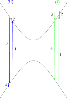
Figure 2: (Color online) Schematic sketch of two types of operator sequences contributing to the four-operator correlation function. Type (i) and (ii) processes are denoted by green and blue, respectively. Indices $1$ to $4$ label the operators from right to left.

Now let us calculate the contribution of two sequences of excitations (i) and (ii). First note that the only terms surviving the trace operation are those proportional to unit $2\times 2$ matrix, and that odd powers of $\sin\varphi$ or $\cos\varphi$ do not survive the angular integration arising from $\sum_{\vec{p}}$. Therefore, the non-zero terms of the first class of terms can be simplified after some algebra as,

$$2\sum_{\cal P}\frac{1}{\beta}\sum_{i\omega_{n}}\int\frac{d^{2}{\vec{p}}}{(2\pi)^{2}}\left[\prod_{\alpha=0}^{3}\frac{1}{z_{\alpha}^{2}-\varepsilon_{\vec{p}}^{2}}\right]\times$$ (16)

$$\frac{p^{2}\cos^{2}\varphi_{\vec{p}}}{\varepsilon_{\vec{p}}^{2}}.\left[\frac{m^{2}\cos^{2}\varphi_{\vec{p}}}{\varepsilon_{\vec{p}}^{2}}+\sin^{2}\varphi_{\vec{p}}\right]\times$$

$$\left[(z_{1}z_{2}+\varepsilon_{\vec{p}}^{2})(z_{0}z_{3}-\varepsilon_{\vec{p}}^{2})+\varepsilon_{\vec{p}}^{2}(z_{1}+z_{2})(z_{0}-z_{3})\right],$$

where frequencies $z_{\alpha},\alpha=0,1,2,3$ are defined in Fig. 1. Similarly for the class (ii) terms we obtain,

$$2\sum_{\cal P}\frac{1}{\beta}\sum_{i\omega_{n}}\int\frac{d^{2}{\vec{p}}}{(2\pi)^{2}}\left[\prod_{\alpha=0}^{3}\frac{1}{z_{\alpha}^{2}-\varepsilon_{\vec{p}}^{2}}\right]\times$$ (17)

$$\frac{p^{2}\cos^{2}\varphi_{\vec{p}}}{\varepsilon_{\vec{p}}^{2}}.\left[\frac{m^{2}\cos^{2}\varphi_{\vec{p}}}{\varepsilon_{\vec{p}}^{2}}+\sin^{2}\varphi_{\vec{p}}\right]\times$$

$$\left[\varepsilon_{\vec{p}}^{2}(z_{2}-z_{3})(z_{0}-z_{1})-(\varepsilon_{\vec{p}}^{2}-z_{2}z_{3})(\varepsilon_{\vec{p}}^{2}-z_{0}z_{1})\right],$$

where an overall factor of $2$ arises from trace over the unit matrix. Adding the above terms gives,

$$2\sum_{\cal P}\frac{1}{\beta}\sum_{i\omega_{n}}\int\frac{d^{2}{\vec{p}}}{(2\pi)^{2}}\left[\prod_{\alpha=0}^{3}\frac{1}{z_{\alpha}^{2}-\varepsilon_{\vec{p}}^{2}}\right]\times$$

$$\frac{p^{2}\cos^{2}\varphi_{\vec{p}}}{\varepsilon_{\vec{p}}^{2}}.\left[\frac{m^{2}\cos^{2}\varphi_{\vec{p}}}{\varepsilon_{\vec{p}}^{2}}+\sin^{2}\varphi_{\vec{p}}\right]\times 2\varepsilon_{\vec{p}}^{2}\times$$

$$\left[z_{0}z_{1}+z_{0}z_{2}-z_{1}z_{2}-\varepsilon_{\vec{p}}^{2}\right].$$ (18)

Now we can evaluate the Matsubara sums, and at the end the result will be symmetrized with respect to exchange of the frequencies of the attached photon vertices. Using the angular averages,

$$\langle\cos^{4}\varphi\rangle=\frac{6}{8},~{}~{}~{}~{}~{}\langle\cos^{2}\varphi~{}\sin^{2}\varphi\rangle=\frac{1}{8},$$ (19)

the angular integration can be simplified to,

$$\sum_{\cal P}\frac{1}{\beta}\sum_{i\omega_{n}}\int\frac{pdp}{2\pi}\left[\prod_{\alpha=0}^{3}\frac{1}{z_{\alpha}^{2}-\varepsilon_{\vec{p}}^{2}}\right]\times$$

$$\frac{p^{2}}{2}\left[6\frac{m^{2}}{\varepsilon_{\vec{p}}^{2}}+1\right]\left[z_{0}z_{1}+z_{0}z_{2}-z_{1}z_{2}-\varepsilon_{\vec{p}}^{2}\right].$$ (20)

Up to this point, the formulation is quite general. At this point, let us specialize to the case of THG, where $i\nu_{1}=i\nu_{2}=i\nu_{3}=i\nu$ and $i\nu_{\sigma}=3i\nu$. In this case, the Feynman diagram shown in Fig. 1 must be labeled with $z_{\alpha}=i\omega_{n}+\alpha i\nu$ for $\alpha=0,1,2,3$. Permuting the external vertices amounts to moving the outgoing $3i\nu$ photon frequency around the loop. Such permutation can be accounted for by a cyclic permutation of the set $\{z_{0},z_{1},z_{2},z_{3}\}$. Performing the $\sum_{\cal P}$ will only affect the last term in Eq. (20) as,

$$\sum_{\cal P}\left[z_{0}z_{1}+z_{0}z_{2}-z_{1}z_{2}-\varepsilon_{\vec{p}}^{2}\right]=2\left[z_{0}z_{2}+z_{1}z_{3}-2\varepsilon_{\vec{p}}^{2}\right],$$

where the THG identification, $z_{\alpha}=i\omega_{n}+\alpha i\nu$ with $\alpha=0,1,2,3$ is understood. Let us emphasize that the above result for the sum over permutation holds only for THG. Therefore the THG susceptibility will become,

$$\chi^{\rm THG} = \frac{1}{\beta}\sum_{i\omega_{n}}\int\frac{pdp}{2\pi}\left[\prod_{\alpha=0}^{3}\frac{1}{z_{\alpha}^{2}-\varepsilon_{\vec{p}}^{2}}\right]\times$$

$$p^{2}\left[6\frac{m^{2}}{\varepsilon_{\vec{p}}^{2}}+1\right]\left[z_{0}z_{2}+z_{1}z_{3}-2\varepsilon_{\vec{p}}^{2}\right]$$

The $1/\beta\sum_{i\omega_{n}}$ can be performed with standard contour integration techniques producing Fermi functions $f(\pm\varepsilon_{\vec{p}})$ corresponding to poles at conduction and valence bands, respectively. Assuming the temperature to be zero, and for undoped massive Dirac spectrum, only contributions from poles at the valence band will be left for which the residues can be calculated to give,

$$\chi^{\rm THG}(\nu_{+}) = \int\frac{pdp}{2\pi}p^{2}\left[6\frac{m^{2}}{\varepsilon_{\vec{p}}^{2}}+1\right]\times$$

$$\frac{3}{2}\frac{4\varepsilon_{\vec{p}}^{2}+\nu_{+}^{2}}{\varepsilon_{\vec{p}}(\nu_{+}^{2}-\varepsilon_{\vec{p}}^{2})(\nu_{+}^{2}-4\varepsilon_{\vec{p}}^{2})(\nu_{+}^{2}-9\varepsilon_{\vec{p}}^{2})}$$

Note that the analytic continuation $i\nu\to\nu_{+}=\nu+i0$ has been performed in the above equation JafariSDW .

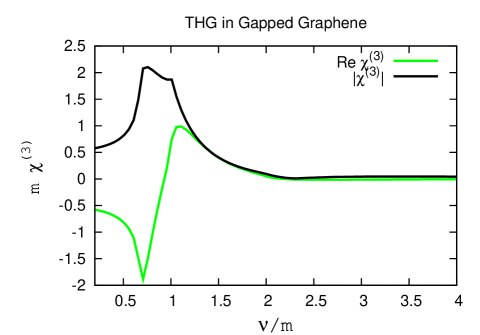
Figure 3: (Color online) THG line-shape for massive Dirac fermions in gapped graphene. The gap parameter $m$ is taken to be unit of energy in this figure. Fundamental constants are assumed to be $e=\hbar=1$.

IV Result and discussions

The radial momentum integration in Eq. (III.2) can be performed with the change of variable to $\varepsilon^{2}=p^{2}+m^{2}$ which gives the following closed form result

$$\chi^{\rm THG}(\nu_{+})=-\frac{m^{3}}{2\pi\nu_{+}^{4}}+\frac{1}{192\pi\nu_{+}^{5}}\times$$

$$\left[-24(6m^{2}+\nu_{+}^{2})(m^{2}-\nu_{+}^{2})\ln\frac{m+\nu_{+}}{m-\nu_{+}}\right.$$

$$+3(4m^{2}-\nu_{+}^{2})(24m^{2}+\nu_{+}^{2})\ln\frac{2m+\nu_{+}}{2m-\nu_{+}}$$

$$\left.+(4m^{2}-9\nu_{+}^{2})(8m^{2}+3\nu_{+}^{2})\ln\frac{2m+3\nu_{+}}{2m-3\nu_{+}}\right]$$ (23)

First of all, note that the above expression when the fundamental constants are restored will be proportional to $e^{4}/\hbar^{3}$. Therefore the above expression shows the results in the natural units. A remarkable feature of the above expression is that, the quantity $m\chi^{\rm THG}$ is only a function of $\nu/m$. This functional form is universal characteristic of 2+1 dimensional Dirac fermions. Hence in Fig. 3, we have plotted the real part and the magnitude of THG line-shape incorporating this observation. This peculiar scaling form indicates that in the limit where $m\to 0$, and the system approaches the gapless limit, since $m\chi^{\rm THG}$ in the natural units employed here will have to remain on the scale of unity, the $\chi^{\rm THG}$ itself will grow inversely proportional to the gap parameter $m$. This sheds a new light into why pristine (gapless) graphene is expected to display large optical nonlinearity Hendry .

Apart from the zero frequency divergence, which is a general feature of optical response functions, an interesting point in the above expression which can be noticed is that, it is precisely the covariant (relativistic) form of the dispersion relation $\varepsilon^{2}=p^{2}+m^{2}$, which after changing integration variables from momentum $p$, to energy $\varepsilon$ leads to logarithmic dependence at finite frequencies $\nu_{\ell}/m=2/\ell$, where $\ell$ is an integer $\ell=1,2,3$. This would not be the case for a typical parabolic dispersion relation in ordinary semiconductors. The main THG peak corresponding to $\ell=1$ and the second one corresponding to $\ell=2$ are clearly seen in the THG spectrum depicted in Fig. 3. The feature corresponding to $\ell=3$ is the weakest feature. Note that as we calculated in Eq. (13), such logarithmic dependence does not show up in the linear optical response. Therefore it can be considered as a valuable information which is contained only in higher order optical responses. Moreover, this logarithmic dependence is not restricted to the THG spectrum, but it also appears in all other higher order responses. To see this, we note in Eq. (20) that in the special case of THG, only the functional form of $\sum_{\cal P}$ as a function of loop frequencies $z_{\alpha}$, will be affected. But the dimensional form of the summand will generally retain a similar form.

The calculation of THG for massive Dirac fermions in 1+1 dimension by Wu Wu indicates a characteristic inverse square root divergence at the main THG peak $\nu_{\ell=1}$ and its harmonics. In the case of small clusters (of correlated 2D nature), a numerical investigation of THG spectrum suggests a line-shape composed of a superposition of resonances corresponding to simple poles Takahashi . For extended 2D system with broken symmetry, it was shown that the nesting underlying spin density wave instability can produce a peculiar $z^{-1/2}\ln(z)$ form of singularity in the non-linear optical spectra JafariSDW . With the above examples in mind, the gapped graphene as a first example of truly two dimensional system provides us with a unique example of a 2D system where optical nonlinearity manifests in a universal logarithmic function of the dimension-less quantity $\nu/m$.

It is interesting to check the limit of gapless graphene by taking the limit $m\to 0$ in Eq. (23), which gives,

$$m\chi^{\rm THG}(\nu)=\frac{54i}{192}\frac{m}{\nu_{+}}$$ (24)

The coefficient of the above expression is universal and can be regarded as a hallmark of the ideal graphene at the THG spectroscopy.

V Acknowledgements

This work was supported by the National Elite Foundation (NEF) of Iran.

References

- (1) K. S. Novoselov, A. K. Geim, S. V. Morozov, D. Jiang, Y. Zhang, S. V. Dubonos, I. V. Grigorieva, and A. A. Firsov, Science 306, 666 (2004); K. S. Novoselov, A. K. Geim, S. V. Morozov, D. Jiang, M. I. Katsnelson, I. V. Grigorieva, S. V. Dubonos, A. A. Firsov, Nature 438, 197 (2005).
- (2) For a review see: A. H. Castro Neto, F. Guinea, N. M. R. Peres, K. S. Novoselov, A. K. Geim, Rev. Mod. Phys. 81, 109 (2009).
- (3) Yu-Ming Lin, Keith A. Jenkins, Alberto Valdes-Garcia, Joshua P. Small, Damon B. Farmer and Phaedon Avouris, Nano. Lett. 9, 422 (2009).
- (4) A. K. Geim, Science 324 1530 (2009).
- (5) Melinda Y. Han, Barbaros Ozyilmaz, Yuanbo Zhang, and Philip Kim, Phys. Rev. Lett. 98, 206805 (2007)
- (6) S. Y. Zhou, G.-H. Gweon, A. V. Fedorov, P. N. First, W. A. de Heer, D.-H. Lee, F. Guinea, A. H. Castro Neto, and A. Lanzara, Nature Materials 6, 770 (2007),
- (7) O. V. Kibis, Phys. Rev. B 81, 165433 (2010).
- (8) G. Bastard, Wave Mechanics Applied to Semiconductor Heterostructures (Les Editions de Physique, Paris, 1988).
- (9) T. Meier, F. Rossi, P. Thomas, and S. W. Koch, Phys. Rev. Lett. 75, 2558 (1995)
- (10) Kin Fai Mak, Matthew Y. Sfeir, Yang Wu, Chun Hung Lui, James A. Misewich, and Tony F. Heinz Phys. Rev. Lett. 101, 196405 (2008).
- (11) Thomas G. Pedersen, Antti-Pekka Jauho, and Kjeld Pedersen, Phys. Rev. B 79, 113406 (2009).
- (12) S. A. Mikhailov and K. Ziegler, J. Phys.: Condens. Matter 20, 384204 (2008).
- (13) A. R. Wright, X. G. Xu, J. C. Cao, and C. Zhang Appl. Phys. Lett. 95, 072101 (2009).
- (14) E. Hendry, P. J. Hale, J. Moger, and A. K. Savchenko, and S. A. Mikhailov Phys. Rev. Lett. 105, 097401 (2010).
- (15) Jun Wang, Yenny Hernandez, Mustafa Lotya, Jonathan N. Coleman, and Werner J. Blau, Adv. Mater, 21, 2430 (2009).
- (16) W. Wu, Phys. Rev. Lett. 61, 1119 (1988).
- (17) V. A. Margulis, T. A. Sizikova, Physica B 245, 173 (1998).
- (18) A. Zarifi, C. Fisker, and T. G. Pedersen, Phys. Rev. B 76 045403 (2007).
- (19) E. A. Desloge, Am. J. Phys. 62, 216 (1994).
- (20) S. A. Jafari, T. Tohyama, S. Maekawa, J. Phys. Soc. Jpn. 75, 054703 (2006).
- (21) S. A. Jafari, Opt. Commun. 282, 317 (2009).
- (22) V. N. Kotov, V. M. Pereira, B. Uchoa, Phys. Rev. B 78, 075433 (2008).
- (23) V. P. Gusynin, S. G. Sharapov, Phys. Rev. B 73, 245411 (2006).
- (24) M. Takahashi, T. Tohyama, S. Maekawa, Phys. Rev. B 66 125102 (2002).