Normally hyperbolic invariant manifolds near strong double resonance

Abstract

In the present paper we consider a generic perturbation of a nearly integrable system of $n$ and a half degrees of freedom

$$H_{\varepsilon}(\theta,p,t)=H_{0}(p)+\varepsilon H_{1}(\theta,p,t),\quad\theta\in\mathbb{T}^{n},\ p\in B^{n},\ t\in\mathbb{T}=\mathbb{R}/\mathbb{Z},$$ (1)

with a strictly convex $H_{0}$. For $n=2$ we show that at a strong double resonance there exist $3$-dimensional normally hyperbolic invariant cylinders going across. This is somewhat unexpected, because at a strong double resonance dynamics can be split into one dimensional fast motion and two dimensional slow motion. Slow motions are described by a mechanical system on a two-torus, which are generically chaotic.

The construction of invariant cylinders involves finitely smooth normal forms, analysis of local transition maps near singular points by means of Shilnikov’s boundary value problem, and Conley–McGehee’s isolating block.

V. Kaloshin     K. Zhang

1 Introduction

Consider the near integrable system from the abstract with $B^{n}\subset\mathbb{R}^{n}$ — the unit ball around $0$, $\mathbb{T}^{n}$ — being the $n$-torus, and $\mathbb{T}$ — the unit circle, respectively. Notice that for $\varepsilon=0$ action component $p$ stays constant. For completely integrable systems coordinates of this form exist and called action-angle. The famous question, called Arnold diffusion, is the following

Conjecture [2, 3] For any two points $p^{\prime},p^{\prime\prime}\in B^{2}$ on the connected level hyper-surface of $H_{0}$ in the action space there exist orbits connecting an arbitrary small neighborhood of the torus $p=p^{\prime}$ with an arbitrary small neighborhood of the torus $p=p^{\prime\prime}$, provided that $\varepsilon\neq 0$ is sufficiently small and that $H_{1}$ is generic.

A proof of this conjecture for $n=2$ is announced by Mather [18].

The classical way to approach this problem is to consider a finite collection of resonances $\Gamma_{1},\ \Gamma_{2},\dots,\Gamma_{N+1}\subset B^{2}$ so that $\Gamma_{1}$ intersects a neighborhood of $p^{\prime}$, $\Gamma_{N+1}$ intersects a neighborhood of $p^{\prime\prime}$, and $\Gamma_{j+1}$ intersects $\Gamma_{j}$ for $j=1,\dots,N$ and diffuse along them. This naive idea faces difficulties at various levels.

Fix an integer relations $\vec{k}_{1}\cdot\partial_{p}H_{0}+k_{0}=0$ with $\vec{k}=(\vec{k}_{1},k_{0})\in(\mathbb{Z}^{2}\setminus 0)\times\mathbb{Z}$ and $\cdot$ being the inner product define one-dimensional resonances. Under the condition that the Hessian of $H_{0}$ is non-degenerate, each resonance defines a smooth curve embedded into the action space $\Gamma_{\vec{k}}=\{p\in B^{2}:\ \vec{k}_{1}\cdot\partial_{p}H_{0}+k_{0}=0\}.$ Such a curve is called a resonance. If one intersects resonances corresponding to two linearly independent $\vec{k}$ and $\vec{k}^{\prime}$ we get isolated points. In the case when both $\vec{k}$ and $\vec{k}^{\prime}$ are relatively small, i.e. $|\vec{k}|,\ |\vec{k}^{\prime}|<K$ for some $K>1$. We call such an intersection a $K$-strong double resonance or simply a strong double resonance (if using $K$ is redundant); see Figure 2. So far only examples of strong double resonances have been studied (see [7, 13, 14, 15]).

1.1 Diffusion along single resonances by means of crumpled normally hyperbolic cylinders

Fix one resonance $\Gamma$. In [6] we prove that depending on a generic $H_{1}$ (but not on $\varepsilon$!) there are a finite number of punctures of $\Gamma$. In other words, there is $K=K(H_{1})>0$ such that way from $\varepsilon^{1/6}$-neighborhood of any $K$-strong double resonance there are diffusing orbits along $\Gamma$. Moreover, these diffusing orbits are constructed in two steps:

• Construct invariant normally hyperbolic invariant cylinders (NHIC) “connecting” a $\varepsilon^{1/6}$-neighborhood of one $K$-strong double resonance with a $\varepsilon^{1/6}$-neighborhood of the next one on $\Gamma$.

• Construct orbits diffusing along these cylinders, which is done using Mather variational method [5, 9, 10].

It turns out that these cylinders are crumpled in the sense that its regularity blows up as $\varepsilon\longrightarrow 0$. See Figure 1. Existence of crumpled NHICs is the new phenomenon, discovered in [6]. In spite of this irregularity, one can use them for diffusion.

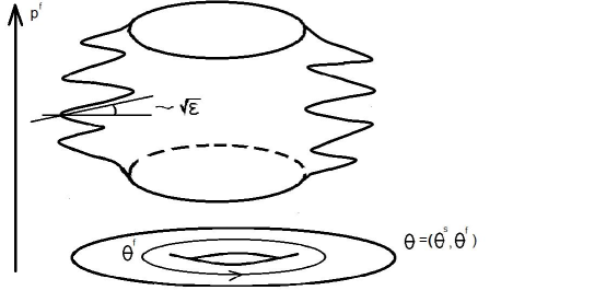
Figure 1: Crumpled Cylinders

The main topic of the present paper is how to diffuse across a strong double resonance. We propose a heuristic description and prove existence of underlying normally hyperbolic invariant manifolds (NHIMs) for it.

1.2 Strong double resonances and slow mechanical systems

We fix two independent resonant lines $\Gamma,\ \Gamma^{\prime}$ and a strong double resonance $p_{0}\in\Gamma\cap\Gamma^{\prime}\subset B^{2}$. Then the standard averaging along the one-dimensional fast direction gives rise to a slow mechanical system $H^{s}=K(I^{s})-U(\theta^{s})$ of two degrees of freedom, where $\theta^{s}\in\mathbb{T}^{s}$ and $I^{s}$ is a rescaled conjugate variable. Namely, in $O(\sqrt{\varepsilon})$-neighborhood of $p_{0}$, after a canonical coordinate change and rescaling the action variables, the flow of the Hamiltonian $H_{\epsilon}$ is conjugate to that of

$$c_{0}/\sqrt{\epsilon}+\sqrt{\epsilon}(K(I^{s})-U(\theta^{s}))+O(\epsilon).$$

Precise definitions of $c_{0}$, $\theta^{s},I^{s}$ are in Section 6.2. The slow kinetic energy $K$ and the slow potential energy $U$ are defined in (10–11), respectively.

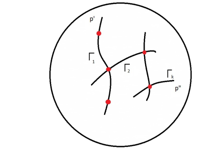
Figure 2: Resonant net

From now on we analyze the slow mechanical system $H^{s}=K(I^{s})-U(\theta^{s})$. Denote by

$$\mathcal{S}_{E}=\{(\theta^{s},I^{s}):\ H^{s}=E\}$$

an energy surface. Without loss of generality assume that the minimum $\min_{\theta^{s}}U(\theta^{s})=0$, it is unique, and occurs at $\theta^{s}=0$. According to the Mapertuis principle for a positive energy $E>0$ orbits of $H^{s}$ restricted to $\mathcal{S}_{E}$ are reparametrized geodesics of the Jacobi metric

$$\rho_{E}(\theta)=2(E+U(\theta))\ K.$$ (2)

Notice that the resonance $\Gamma\subset B^{2}$ (resp. $\Gamma^{\prime}\subset B^{2}$) induces an integer homology class $h$ (resp. $h^{\prime}$) on $\mathbb{T}^{s}$, i.e. $h$ (resp. $h^{\prime}$) $\in H_{1}(\mathbb{T}^{s},\mathbb{Z})$. Denote by $\gamma_{h}^{E}$ (resp. $\gamma_{h^{\prime}}^{E}$) a minimal geodesic of $\rho_{E}$ in the homology class $h$ (resp. $h^{\prime}$). For example, if $H_{\varepsilon}(\theta,p,t)=\dfrac{1}{2}p^{2}+\varepsilon H_{1}(\theta,p,t)$, $\Gamma=\{p:\ \partial_{p_{2}}H_{0}=p_{2}=0\}$ (resp. $\Gamma^{\prime}=\{p:\ \partial_{p_{1}}H_{0}=p_{1}=0\}$). Then on the slow torus $\mathbb{T}^{s}\ni(p_{1},p_{2})$ we have $h=(1,0)$ (resp. $h^{\prime}=(0,1)$). On the unit energy surface $S_{1}$ the strong resonance occurs at $p_{0}=(0,0,1)\in\Gamma\cap\Gamma^{\prime}$.

1.3 Two types of NHIMs at a strong double resonance

Notice that diffusing along $\Gamma$ for the Hamiltonian $H$ corresponds to changing slow energy $E$ of $H^{s}$ along the homology class $h$. In particular, we need to get across zero energy. However, $\mathcal{S}_{0}=\{(\theta^{s},I^{s}):\ H^{s}=0\}$ is the critical energy surface, namely, the Jacobi metric is degenerate at the origin.

There are at least two special integer homology classes $h_{1},h_{2}\in H_{1}(\mathbb{T}^{s},\mathbb{Z})$ such that minimal geodesics of $g_{0}$ are non-self-intersecting. For $i=1,2$, we denote by $\gamma_{E}^{-h_{i}}$ the curve obtained by the time reversal $I^{s}\longrightarrow-I^{s}$ and $t\longrightarrow-t$. Then

$$\textit{ the union of }\gamma_{E}^{\pm h_{i}}\textit{ over }0\leq E\leq E_{0}\textit{ is contained in a }$$ (3)

$$C^{1}\textit{ smooth two-dimensional NHIM }\mathcal{M}_{h_{i}}.$$

This imply that the original Hamiltonian system $H_{\varepsilon}$ also has two three-dimensional NHIM $C^{1}$-close to $\mathcal{M}_{h_{1}}$ and $\mathcal{M}_{h_{2}}$. By the reason to be clear later we call such cylinders simple loop cylinders.

Moreover, for small $E_{0}>0$ and all energies $E_{0}<E<E_{0}^{-1}$ except finitely many $\{E_{j}\}_{j=1}^{N}\subset[E_{0},E_{0}^{-1}],E_{j}<E_{j+1},j=1,\dots,N-1$ we show that for each $1\leq j\leq N$ a proper union $\mathcal{M}^{h}_{j}$ of $\gamma_{E}^{h}$ over $E_{j}<E<E_{j+1}$ form $C^{1}$ smooth NHIC. This imply that the original Hamiltonian system $H_{\varepsilon}$ also has a NHIC $C^{1}$-close to $\mathcal{M}^{h}$. See the Appendix for more details.

1.3.1 Non-simple figure $8$ loops

If minimal geodesics of $\rho_{0}$ are self-intersecting the situation was described by Mather [21]. Generically $\gamma^{E}_{h}$ accumulates onto the union of two simple loops, possibly with multiplicities. More precisely, given $h\in H_{1}(\mathbb{T}^{s},\mathbb{Z})$ generically there are homology classes $h_{1},\ h_{2}\in H_{1}(\mathbb{T}^{s},\mathbb{Z})$ and integers $n_{1},\ n_{2}\in\mathbb{Z}_{+}$ such that the corresponding minimal geodesics $\gamma_{0}^{h_{1}}$ and $\gamma_{0}^{h_{2}}$ are simple and $h=n_{1}h_{1}+n_{2}h_{2}$. Denote $n=n_{1}+n_{2}$.

For $E>0$, $\gamma^{h}_{E}$ has no self intersection. As a consequence, there is a unique way to represent $\gamma_{h}^{0}$ as a concatenation of $\gamma^{h_{1}}_{0}$ and $\gamma^{h_{2}}_{0}$. More precisely, we have the following lemma.

Lemma 1.1.

There exists a sequence $\sigma=(\sigma_{1},\cdots,\sigma_{n})\in\{1,2\}^{n}$, unique up to cyclical translation, such that

$$\gamma^{h}_{0}=\gamma^{h_{\sigma_{1}}}_{0}*\cdots*\gamma^{h_{\sigma_{n}}}_{0}.$$

Lemma 1.1 will be proved in Appendix B. In this case for small energies this cylinder resembles the figure $8$ and we call it two leaf cylinder and call the corresponding $\gamma^{h}_{0}$ non-simple.

We would like to point out that Jean-Pierre Marco [16, 17] is studying similar ideas.

1.3.2 Kissing cylinders

If the loop $\gamma^{h}_{0}$ is non-simple, then the union $\mathcal{M}_{h}^{8}=\bigcup_{0\leq E\leq E_{0}}\gamma^{h}_{E}$ is not a manifold at $\gamma_{h}^{0}$! However, $\mathcal{M}_{h_{1}},\mathcal{M}_{h_{2}},$ and $\mathcal{M}_{h}^{8}$ all have a tangency at the origin (see Remark 1.1). Moreover, expanding and contracting directions at the origin of all the three normally hyperbolic invariant manifolds are parallel to strong unstable and strong stable directions. Simple dimension consideration makes us believe that for the original Hamiltonian $H_{\varepsilon}$ has NHIMs $\mathcal{M}^{\varepsilon}_{h_{1}},\mathcal{M}^{\varepsilon}_{h_{2}},\mathcal{M}^{8}_{h}$ with transversal intersections of invariant manifolds.

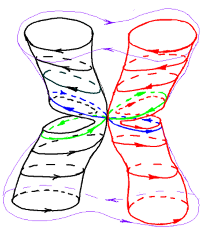
Figure 3: Kissing Cylinders

1.4 An heuristic diffusion through strong double resonances

We hope the following mechanism of diffusion through double resonance takes place. As we mentioned above in [6] we show that away from $\varepsilon^{1/6}$-neighborhood of strong double resonances there are crumpled NHIC and orbits diffusing along them. It turns out that in the region where distance to the center of a strong double resonance is between $[\varepsilon^{a},\varepsilon^{1/6}]$ for some $1/6<a<1/2$ we can slightly modify argument from [6] and show that the system $H_{\varepsilon}(\theta,p,t)$ has a NHIC. Moreover, this cylinder is smoothly attached to the crumpled NHICs build in [6].

1.4.1 First intermediate zone

Fix $C=C(H_{0},H_{1})\gg 1$, but independent of $\varepsilon$. In the region where distance to the center of a strong double resonance is between $[C\sqrt{\varepsilon},\varepsilon^{a}]$ we define a slow-fast mechanical system and show that it approximates dynamics of our system $H_{\varepsilon}(\theta,p,t)$ well enough to establish existence of a NHIC. Moreover, this cylinder is smoothly attached to the one from the region $[\varepsilon^{a},\varepsilon^{1/6}]$.

1.4.2 Second intermediate zone

Let $C=E_{0}^{-1}$. Consider the region where distance to the center of a strong double resonance is between $[E_{0}\sqrt{\varepsilon},E_{0}^{-1}\sqrt{\varepsilon}]$. In this regime dynamics is well approximable by a slow mechanical system. Thus, we need to study a mechanical system of two degrees of freedom on an interval of energy surfaces and its family of minimal geodesics $\{\gamma_{E}^{h}\}_{E}$ in a given homology class $h\in H_{1}(\mathbb{T}^{s},\mathbb{Z})$. The left boundary $E_{0}\sqrt{\varepsilon}$ means that we need to study a mechanical system for slow energies $E>E_{0}$.

Simple analysis, carried out in Appendix A, shows that and all energies $E_{0}<E<E_{0}^{-1}$ except finitely many $\{E_{j}\}_{j=1}^{N}\subset[E_{0},E_{0}^{-1}],\ E_{j}<E_{j+1},\ j=1,\dots,N-1$ a proper union $\mathcal{M}^{h}_{j}$ of $\gamma_{E}^{h}$ over $E_{j}<E<E_{j+1}$ form $C^{1}$ smooth NHIC. Application of Conley–McGehee’s isolating block implies that the original Hamiltonian system $H_{\varepsilon}$ also has a NHIC $C^{1}$-close to $\mathcal{M}^{h}_{j}$. Moreover, one can construct diffusing orbits along $\{\mathcal{M}^{h}_{j}\}_{j=1}^{N-1}$. This part is very much analogous to the one done in [6].

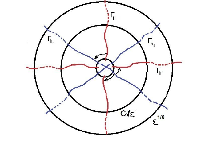
Figure 4: Heuristic description

Now we arrive to slow energy $E_{0}\sqrt{\varepsilon}$ near a strong double resonance and need to consider several cases. Heuristic description of our mechanism is on Figure 4. First, we cross a strong double resonance along $\Gamma$.

1.4.3 Crossing through along a simple loop $\Gamma$

If $\gamma^{h}_{0}$ is simple or does not pass through the origin at all, then an orbit enters along a NHIC $\mathcal{M}^{h}_{1}$ and can diffuse along NHIM $\mathcal{M}_{h}$ across the center of a strong double resonance $p_{0}$ to “the other side”.

1.4.4 Crossing through along a non-simple $\Gamma$

If $\gamma^{h}_{0}$ is non-simple, i.e the union of two simple loops, then an orbit enters along a NHIC $\mathcal{M}^{h}_{1}$. As it diffuses toward the center of a strong double resonance $p_{0}$ the cylinder $\mathcal{M}_{h}^{8}$ becomes a two leaf cylinder and its boundary approaches the figure $8$.

For a small enough energy $\delta>0$ of the mechanical system $H^{s}$ the two leaf cylinder $\mathcal{M}_{h}^{8}$ is almost tangent to a certain simple loop NHIC $\mathcal{M}_{h_{i}}$. Moreover, near the origin both of normally hyperbolic invariant manifolds have almost parallel most contract and expanding directions. As a result there should be orbits jumping from the two leaf cylinder $\mathcal{M}_{h}^{8}$ to a simple loop one $\mathcal{M}_{h_{i}}$ from (3). Then such orbits can cross the double resonance along $\mathcal{M}_{h_{i}}$. After that it jumps back on the opposite branch of $\mathcal{M}_{h}^{8}$ and diffuse away along $\Gamma$ as before.

1.4.5 Turning a corner from $\Gamma$ to $\Gamma^{\prime}$

Now we cross a strong double resonance by entering along $\Gamma$ and exiting along $\Gamma^{\prime}$. As before an orbit enters along a NHIC $\mathcal{M}^{h}_{1}$ constructed in the second intermediate zone. As it diffused toward the center of a strong double resonance $p_{0}$ the cylinder $\mathcal{M}_{h}^{8}$ becomes a two leaf cylinder.

As in the previous case if we diffuse along $\mathcal{M}_{h}^{8}$ to a small enough energy.

• If $h^{\prime}$ has a simple loop $\gamma^{h^{\prime}}_{0}$, then we jump to $\mathcal{M}_{h^{\prime}}$ directly from $\mathcal{M}_{h}^{8}$ and cross the strong double resonance along $\mathcal{M}_{h^{\prime}}$.

• If $h^{\prime}$ is non-simple, then $\mathcal{M}_{h^{\prime}}^{8}$ also becomes a double leaf cylinder. In this case we first jump onto a simple loop cylinder $\mathcal{M}_{h_{i}}$, cross the double resonance, and only afterward jump onto $\mathcal{M}_{h^{\prime}}^{8}$.

To summarize we expect that crumpled NHICs from [6] can be continued from a $\varepsilon^{1/6}$-neighborhood of $p_{0}$ to $C\sqrt{\varepsilon}$-neighborhood and can be used for diffusion. Thus, we distinguish two essentially different regions: ($C\sqrt{\varepsilon}$-)near a strong double resonance and ($C\sqrt{\varepsilon}$-)away from it. The main focus of this paper is the first case.

1.5 Formulation of the main results (small energy)

The case of finite non-small energies is treated in Appendix A. We will formulate our main results in terms of the slow mechanical system

$$H^{s}(I^{s},\theta^{s})=K(I^{s})-U(\theta^{s}).$$ (4)

We make the following assumptions:

1. The potential $U$ has a unique non-degenerate minimum at $0$ and $U(0)=0$.

2. The linearization of the Hamiltonian flow at $(0,0)$ has distinct eigenvalues $-\lambda_{2}<-\lambda_{1}<0<\lambda_{1}<\lambda_{2}$

In a neighborhood of $(0,0)$, there exists a local coordinate system $(u_{1},u_{2},s_{1},s_{2})=(u,s)$ such that the $u_{i}-$axes correspond to the eigendirections of $\lambda_{i}$ and the $s_{i}-$ axes correspond to the eigendirections of $-\lambda_{i}$ for $i=1,2$. Let $\gamma^{+}$ and $\gamma^{-}$ be two homoclinic orbits of $(0,0)$ under the Hamiltonian flow of $H^{s}$. This setting applies to the case of a simple loop cylinder, with $\gamma^{+}=\gamma_{0}^{h,+}$ and $\gamma^{-}$ being the time reversal of $\gamma_{0}^{h,+}$, denoted $\gamma_{0}^{h,-}$, (which is the image of $\gamma_{0}^{h,+}$ under the involution $I^{s}\mapsto-I^{s}$ and $t\mapsto-t$). We call $\gamma^{+}$ (resp. $\gamma^{-}$) simple loop.

We assume the following of the homoclinics $\gamma^{+}$ and $\gamma^{-}$.

1. The homoclinics $\gamma^{+}$ and $\gamma^{-}$ are not tangent to $u_{2}-$axis or $s_{2}-$axis at $(0,0)$. This, in particular, imply that the curves are tangent to the $u_{1}$ and $s_{1}$ directions. We assume that $\gamma^{+}$ approaches $(0,0)$ along $s_{1}>0$ in the forward time, and approaches $(0,0)$ along $u_{1}>0$ in the backward time; $\gamma^{-}$ approaches $(0,0)$ along $s_{1}<0$ in the forward time, and approaches $(0,0)$ along $u_{1}<0$ in the backward time.

For the case of the double leaf cylinder, we consider two homoclinics $\gamma_{1}$ and $\gamma_{2}$ that are in the same direction instead of being in the opposite direction. More precisely, the following is assumed.

1. The homoclinics $\gamma_{1}$ and $\gamma_{2}$ are not tangent to $u_{2}-$axis or $s_{2}-$axis at $(0,0)$. Both $\gamma_{1}$ and $\gamma_{2}$ approaches $(0,0)$ along $s_{1}>0$ in the forward time, and approaches $(0,0)$ along $u_{1}>0$ in the backward time.

Given $r>0$ and $0<\delta<r$, let $B_{r}$ be the $r-$neighborhood of $(0,0)$ and let

$$\Sigma^{s}_{\pm}=\{s_{1}=\pm\delta\}\cap B_{r},\quad\Sigma^{u}_{\pm}=\{u_{1}=\pm\delta\}\cap B_{r}$$

be four local sections contained in $B_{r}$. We have four local maps

$$\Phi_{\mathrm{loc}}^{++}:U^{++}(\subset\Sigma^{s}_{+})\longrightarrow\Sigma^{u}_{+},\qquad\Phi_{\mathrm{loc}}^{-+}:U^{-+}(\subset\Sigma^{s}_{-})\longrightarrow\Sigma^{u}_{+},$$

$$\Phi_{\mathrm{loc}}^{+-}:U^{+-}(\subset\Sigma^{s}_{+})\longrightarrow\Sigma^{u}_{-},\qquad\Phi_{\mathrm{loc}}^{--}:U^{--}(\subset\Sigma^{s}_{-})\longrightarrow\Sigma^{u}_{-}.$$

The local maps are defined in the following way. Let $(u,s)$ be in the domain of one of the local maps. If the orbit of $(u,s)$ escapes $B_{r}$ before reaching the destination section, then the map is considered undefined there. Otherwise, the local map maps $(u,s)$ to the first intersection of the orbit with the destination section. The local map is not defined on the whole section and its domain will be made precise later.

For the case of simple loop cylinder, i.e. assume A3, we can define two global maps corresponding to the homoclinics $\gamma^{+}$ and $\gamma^{-}$. By assumption A3, for a sufficiently small $\delta$, the homoclinic $\gamma^{+}$ intersects the sections $\Sigma^{u,s}_{+}$ and $\gamma^{-}$ intersects $\Sigma^{u,s}_{-}$. Let $p^{+}$ and $q^{+}$ (resp. $p^{-}$ and $q^{-}$) be the intersection of $\gamma^{+}$ (resp. $\gamma^{-}$) with $\Sigma^{u}_{+}$ and $\Sigma^{s}_{+}$ (resp. $\Sigma^{u}_{-}$ and $\Sigma^{s}_{-}$) . Smooth dependence on initial conditions implies that for the neighborhoods $V^{\pm}\ni q^{\pm}$ there are a well defined Poincaré return maps

$$\Phi_{\mathrm{glob}}^{+}:V^{+}\longrightarrow\Sigma^{s}_{+},\qquad\Phi_{\mathrm{glob}}^{-}:V^{-}\longrightarrow\Sigma^{s}_{-}.$$

When A$3^{\prime}$ is assumed, for $i=1,2$, $\gamma^{i}$ intersect $\Sigma^{u}_{+}$ at $q^{i}$ and intersect $\Sigma^{s}_{+}$ at $p^{i}$. The global maps are denoted

$$\Phi_{\mathrm{glob}}^{1}:V^{1}\longrightarrow\Sigma^{s}_{+},\qquad\Phi_{\mathrm{glob}}^{2}:V^{1}\longrightarrow\Sigma^{s}_{+}.$$

Figure 5: Global and local maps for $\gamma^{+}$

The composition of local and global maps for the periodic orbits shadowing $\gamma^{+}$ is illustrated in Figure 5.

We will assume that the global maps are “in general position”. We will only phrase our assumptions A4a and A4b for the homoclinic $\gamma^{+}$ and $\gamma^{-}$. The assumptions for $\gamma^{1}$ and $\gamma^{2}$ are identical, only requiring different notations and will be called A4a^′ and A4b^′. Let $W^{s}$ and $W^{u}$ denote the local stable and unstable manifolds of $(0,0)$. Note that $W^{u}\cap\Sigma^{u}_{\pm}$ is one-dimensional and contains $q^{\pm}$. Let $T^{uu}(q^{\pm})$ be the tangent direction to this one dimensional curve at $q^{\pm}$. Similarly, we define $T^{ss}(p^{\pm})$ to be the tangent direction to $W^{s}\cap\Sigma^{s}_{\pm}$ at $p^{\pm}$.

1. Image of strong stable and unstable directions under $D\Phi_{\mathrm{glob}}^{\pm}(q^{\pm})$ is transverse to strong stable and unstable directions at $p^{\pm}$ on the energy surface $S_{0}=\{H^{s}=0\}$. For the restriction to $S_{0}$ we have

   $$D\Phi_{\mathrm{glob}}^{+}(q^{+})|_{TS_{0}}T^{uu}(q^{+})\pitchfork T^{ss}(p^{+}),\quad D\Phi_{\mathrm{glob}}^{-}(q^{-})|_{TS_{0}}T^{uu}(q^{-})\pitchfork T^{ss}(p^{-}).$$

2. Under the global map, the image of the plane $\{s_{2}=u_{1}=0\}$ intersects $\{s_{1}=u_{2}=0\}$ at a one dimensional manifold, and the intersection transversal to the strong stable and unstable direction. More precisely, let

   $$L(p^{\pm})=D\Phi_{\mathrm{glob}}^{\pm}(q^{\pm})\{s_{2}=u_{1}=0\}\cap\{s_{1}=u_{2}=0\},$$

   we have that $\dim L(p^{\pm})=1$, $L(p^{\pm})\neq T^{ss}(p^{\pm})$ and $D(\Phi_{\mathrm{glob}}^{\pm})^{-1}L(p^{\pm})\neq T^{uu}(q^{\pm})$.

3. Suppose conditions A4a and A4b hold for both $\gamma_{1}$ and $\gamma_{2}$.

We show that under our assumptions, for small energy, there exists “shadowing” periodic orbits close to the homoclinics. These orbits were studied by Shil’nikov [23], Shil’nikov-Turaev [25], and Bolotin-Rabinowitz [8].

Theorem 1.1.

1. In the simple loop case, we assume that the assumptions A1 - A4 hold for $\gamma^{+}$ and $\gamma^{-}$. Then there exists $E_{0}>0$ such that for each $0<E\leq E_{0}$, there exists a periodic orbit $\gamma_{E}^{+}$ corresponding to a fixed point of the map $\Phi_{\mathrm{glob}}^{+}\circ\Phi_{\mathrm{loc}}^{++}$ restricted to the energy surface $\mathcal{S}_{E}$.

   For each $-E_{0}\leq E<0$, there exists a periodic orbit $\gamma^{c}_{E}$ corresponding to a fixed point of the map $\Phi_{\mathrm{glob}}^{-}\circ\Phi_{\mathrm{loc}}^{+-}\circ\Phi_{\mathrm{glob}}^{+}\circ\Phi_{\mathrm{loc}}^{-+}$ restricted to the energy surface $\mathcal{S}_{E}$.

   For each $0<E\leq E_{0}$, there exists a periodic orbit $\gamma_{E}^{-}$ corresponding to a fixed point of the map $\Phi_{\mathrm{glob}}^{-}\circ\Phi_{\mathrm{loc}}^{--}$ restricted to the energy surface $\mathcal{S}_{E}$.

2. In the non-simple case, assume that the assumptions A1, A2, A3$\,{}^{\prime}$ and A4^′ hold for $\gamma^{1}$ and $\gamma^{2}$. Then there exists $E_{0}>0$ such that for $0<E\leq E_{0}$, the following hold. For any $\sigma=(\sigma_{1},\cdots,\sigma_{n})$, there is a periodic orbit $\gamma^{\sigma}_{E}$ corresponding to a fixed point of the map

   $$\prod_{i=n}^{1}\left(\Phi_{\mathrm{glob}}^{\sigma_{i}}\circ\Phi_{\mathrm{loc}}^{++}\right)$$

   restricted to the energy surface $\mathcal{S}_{E}$. (Product stands for composition of maps).

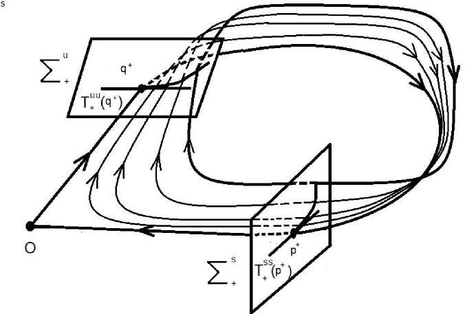
Figure 6: Periodic orbits shadowing $\gamma^{+}$

The the periodic orbits $\gamma^{+}_{E}$ are depicted in Figure 6.

Theorem 1.2.

In the case of simple loop, assume that A1-A4 are satisfied with $\gamma^{+}=\gamma^{h,+}_{0}$ and $\gamma^{-}=\gamma^{h,-}_{0}$. For this choice of $\gamma^{+}$ and $\gamma^{-}$, let $\gamma^{+}_{E}$, $\gamma^{c}_{E}$ and $\gamma^{-}_{E}$ be the periodic orbits obtained from part 1 of Theorem 1.1 .

$$\mathcal{M}_{h}^{E_{0}}=\bigcup_{0<E\leq E_{0}}\gamma^{+}_{E}\cup\gamma\cup\bigcup_{-E_{0}\leq E<0}\gamma^{c}_{E}\cup\gamma^{-}\cup\bigcup_{0<E\leq E_{0}}\gamma^{-}_{E}$$

is a $C^{1}$ smooth normally hyperbolic invariant manifold with boundaries $\gamma^{+}_{E_{0}}$, $\gamma^{c}_{E_{0}}$ and $\gamma^{-}_{E_{0}}$.

In the case of non-simple loop, assume that A1, A2, A3 ^′ and A4^′ are satisfied with $\gamma^{1}=\gamma^{h_{1}}_{0}$ and $\gamma^{2}=\gamma^{h_{2}}_{0}$. Let $\gamma^{\sigma}_{E}$ denote the periodic orbits obtained from applying part 2 of Theorem 1.1 to the sequence $\sigma$ determined by Lemma 1.1. We have that for any $e>0$, the set

$$\mathcal{M}_{h}^{e,E_{0}}=\cup_{e\leq E\leq E_{0}}\gamma^{\sigma}_{E}$$

is a $C^{1}$ smooth normally hyperbolic invariant manifold.

Remark 1.1.

Due to hyperbolicity the cylinder $\mathcal{M}_{h}^{E_{0}}$ is $C^{\alpha}$ for any $0<\alpha<\lambda_{2}/\lambda_{1}$.

If $h_{1}$ and $h_{2}$ corresponds to simple loops, then the corresponding invariant manifolds $\mathcal{M}_{h_{1}}^{E_{0}}$ and $\mathcal{M}_{h_{2}}^{E_{0}}$ have a tangency along a two dimensional plane at the origin. One can say that we have “kissing manifolds”, see Figure 3.

Remark 1.2.

In the simple loop case, we expect the shadowing orbits $\gamma^{\pm}_{E}$, for $0\leq E\leq E_{0}$ to coincide with the minimal geodesics $\gamma^{\pm h}_{E}$. In the non-simple case, $\gamma^{\sigma}_{E}$ should coincide with $\gamma_{E}^{h}$ for $0\leq E\leq E_{0}$ (by Lemma 1.1, $\sigma$ is uniquely determined by $h$). The proof is not included in this paper, as we only deal with the geometrical part of the diffusion.

Corollary 1.2.

The system $H_{\varepsilon}$ has a normally hyperbolic manifold $\mathcal{M}_{h,\varepsilon}^{E_{0}}$ (resp. $\mathcal{M}_{h,\varepsilon}^{e,E_{0}}$) which is weakly invariant, i.e. the Hamiltonian vector field of $H_{\varepsilon}$ is tangent to $\mathcal{M}_{h,\varepsilon}^{E_{0}}$ (resp. $\mathcal{M}_{h,\varepsilon}^{e,E_{0}}$). Moreover, the intersection of $\mathcal{M}_{h,\varepsilon}^{E_{0}}$ (resp. $\mathcal{M}_{h,\varepsilon}^{e,E_{0}}$) with the regions $\{-E_{0}\leq H^{s}\leq E_{0}\}\times\mathbb{T}$ (resp. $\{e\leq H^{s}\leq E_{0}\}\times\mathbb{T}$) is a $C^{1}$-graph over $\mathcal{M}_{h}^{E_{0}}$ (resp. $\mathcal{M}_{h}^{e,E_{0}}$).

Proof of Corollary 1.2 is included in section 6.3.

2 Normal form near the hyperbolic fixed point

In a neighborhood of the origin, there exists a a symplectic linear change of coordinates under which the system has the normal form

$$H(u_{1},u_{2},s_{1},s_{2})=\lambda_{1}s_{1}u_{1}+\lambda_{2}s_{2}u_{2}+O_{3}(s,u).$$

Here $s=(s_{1},s_{2})$, $u=(u_{1},u_{2})$, and $O_{n}(s,u)$ stands for a function bounded by $C|(s,u)|^{n}$. According to our assumptions, $\lambda_{1}<\lambda_{2}$.

The main result of this section is the following normal form

Theorem 2.1.

There exists $k\in\mathbb{N}$ depending only on $\lambda_{2}/\lambda_{1}$ such that if $H$ is $C^{k+1}$, the following hold. There exists neighborhood $U$ of the origin and a $C^{2}$ change of coordinates $\Phi$ on $U$ such that $N_{k}=H\circ\Phi$ has the form is a polynomial of degree $k$ of the form

$$\begin{bmatrix}\dot{s}_{1}\\ \dot{s}_{2}\\ \dot{u}_{1}\\ \dot{u}_{2}\end{bmatrix}=\begin{bmatrix}-\partial_{u_{1}}N_{k}\\ -\partial_{u_{2}}N_{k}\\ \partial_{s_{1}}N_{k}\\ \partial_{s_{2}}N_{k}\end{bmatrix}=\begin{bmatrix}-\lambda_{1}s_{1}+F_{1}(s,u)\\ -\lambda_{2}s_{2}+F_{2}(s,u)\\ \ \ \lambda u_{1}+G_{1}(s,u)\\ \ \ \lambda u_{2}+G_{2}(s,u)\end{bmatrix}$$ (5)

where

$$F_{1}=s_{1}O_{1}(s,u)+s_{2}O_{1}(s,u),\quad F_{2}=s_{1}^{2}O(1)+s_{2}O_{1}(s,u),$$

$$G_{1}=u_{1}O_{1}(s,u)+u_{2}O_{1}(s,u),\quad G_{2}=u_{1}^{2}O(1)+u_{2}O_{1}(s,u).$$

The proof consists of two steps: first, we do some preliminary normal form and then apply a theorem of Belitskii-Samovol (See, for example [12]).

Since $(0,0)$ is a hyperbolic fixed point, for sufficiently small $r>0$, there exists stable manifold $W^{s}=\{(u=U(s),|s|\leq r\}$ and unstable manifold $W^{u}=\{s=S(u),|u|\leq r\}$ containing the origin. All points on $W^{s}$ converges to $(0,0)$ exponentially in forward time, while all points on $W^{u}$ converges to $(0,0)$ exponentially in backward time. These manifolds are Lagrangian; as a consequence, the change of coordinates $s^{\prime}=s-S(u)$, $u^{\prime}=u-U(s^{\prime})=u-U(s-S(u))$ is symplectic. Under the new coordinates, we have that $W^{s}=\{u^{\prime}=0\}$ and $W^{u}=\{s^{\prime}=0\}$. We abuse notation and keep using $(s,u)$ to denote the new coordinate system.

Under the new coordinate system, the Hamiltonian has the form

$$H(s,u)=\lambda_{1}s_{1}u_{1}+\lambda_{2}s_{2}u_{2}+H_{1}(s,u),$$

where $H(s,u)=O_{3}(s,u)$ and $H_{1}(s,u)|_{s=0}=H_{1}(s,u)|_{u=0}=0$. Let us denote $H_{0}=\lambda_{1}s_{1}u_{1}+\lambda_{2}s_{2}u_{2}$. We now perform a further step of normalization.

We say an tuple $(\alpha,\beta)\in\mathbb{N}^{2}\times\mathbb{N}^{2}$ is resonant if $\sum_{i=1}^{2}\lambda_{i}(\alpha_{i}-\beta_{i})=0.$ Note that an $(\alpha,\beta)$ with $\alpha_{i}=\beta_{i}$ for $i=1,2$ is always resonant. A monomial $u_{1}^{\alpha_{1}}u_{2}^{\alpha_{2}}s_{1}^{\beta_{1}}s_{2}^{\beta_{2}}$ is resonant if $(\alpha,\beta)$ is resonant. Otherwise, we call it nonresonant. It is well known that a Hamiltonian can always be transformed, via a formal power series, to an Hamiltonian with only resonant terms.

Proposition 2.2.

If $H$ is at least $C^{k+1}$, the there exists a $C^{\infty}-$symplectic change of coordinates $(s,u)=\Phi(s^{\prime},u^{\prime})$ defined on a neighborhood of $(0,0)$ such that

$$H\circ\Phi^{\prime}=N_{k}(s^{\prime},u^{\prime})+H_{2}(s^{\prime},u^{\prime}),$$

where $N_{k}$ is a polynomial of degree $k$ consisting only of resonant terms and $H_{2}=O_{k+1}(s^{\prime},u^{\prime})$.

Proof.

Let $S_{k}$ denote the set of all nonresonant indices $(\alpha,\beta)\in\mathbb{N}^{2}\times\mathbb{N}^{2}$ with $|\alpha|+|\beta|=k$. We define the change of coordinates by the generating function

$$G_{k}(s,u^{\prime})=s_{1}u_{1}^{\prime}+s_{2}u_{2}^{\prime}+\sum_{3\leq i\leq k+1}\sum_{(\alpha,\beta)\in S_{i}}g_{\alpha,\beta}s^{\alpha}(u^{\prime})^{\beta}.$$

The symplectic change of coordinates is defined by $s^{\prime}=\partial_{u^{\prime}}G_{k}$ and $u=\partial_{s}G_{k}$. Assume that

$$H\circ\Phi=\sum_{i\geq 2}\sum_{|\alpha|+|\beta|}h_{\alpha,\beta}(s^{\prime})^{\alpha}(u^{\prime})^{\beta}.$$

We have that if $(\alpha,\beta)$ is nonresonant, there exists a unique $g_{\alpha,\beta}$ such that $h_{\alpha,\beta}=0$ (see [24], section 30, for example). By choosing $g_{\alpha,\beta}$ appropriately, we obtain the desired normal form. ∎

We abuse notations by replacing $(s^{\prime},u^{\prime})$ with $(s,u)$. Using our assumption that $0<\lambda_{1}<\lambda_{2}$, we have that all $(\alpha,\beta)$ with $\alpha\neq\beta$, $\alpha_{1}=1$ and $\alpha_{2}=0$ are nonresonant, and similarly, all $(\alpha,\beta)$ with $\alpha\neq\beta$, $\beta_{1}=1$ and $\beta_{2}=0$ are nonresonant. Furthermore, by performing the straightening of stable/unstable manifolds again if necessary, we may assume that $N_{k}|_{s=0}=N_{k}|_{u=0}=0$. As a consequence, the normal form $N_{k}$ must take the following form:

Corollary 2.1.

The normal form $N_{k}$ satisfies

$$N_{k}=\lambda_{1}s_{1}u_{1}+\lambda_{2}s_{2}u_{2}+s_{2}O_{1}(u)O_{1}(s,u)+s_{1}^{2}O_{1}(u)+u_{2}O_{1}(s)O_{1}(s,u)+u_{1}^{2}O_{1}(s)$$

In particular, we have $N_{k}=\lambda_{1}s_{1}u_{1}+\lambda_{2}s_{2}u_{2}+O_{3}(s,u)$.

Under the normal form the equations of motion is

$$\begin{cases}\dot{s}=-\partial_{u}N_{k}+O_{k}(s,u)\\ \dot{u}=\partial_{s}N_{k}+O_{k}(s,u)\end{cases}.$$ (6)

As the linearization of these equations is hyperbolic, for sufficiently large $r$ it is possible to kill the small remainder with a finitely smooth change of coordinates.

Theorem 2.1 is a direct consequence of the following theorem:

Theorem 2.3 (Belitskii-Samovol).

(See [12], Chapter 6, Theorem 1.6) For any $l\in\mathbb{N}$ and $\lambda\in\mathbb{C}^{n}$ with $Re\lambda_{i}\neq 0$, there exists an integer $k=k(l,\lambda)$ such that the following hold. Suppose two germs of vector fields at a hyperbolic fixed point with the spectrum of linearization equal to $\lambda$, and their jets of order $k$ coincide at the fixed point. Then the two vector fields are $C^{l}-$conjugate.

3 Behavior of a family of orbits passing near $0$ and Shil’nikov boundary value problem

The main result of this section is the following

Theorem 3.1.

Let $(s^{T},u^{T})$ be a family of orbits satisfying $s^{T}(0)\longrightarrow s^{in}$ as $T\longrightarrow\infty$ with $s_{1}^{T}=\delta$ and $u^{T}(T)\longrightarrow u^{out}$ as $T\longrightarrow\infty$ with $s_{1}^{T}=\delta$ with $|s^{T}|,|u^{T}|\leq 2\delta$, where $\delta$ is small enough. Then there exists $T_{0},\ C>0$ and $\alpha>1$ such that for each $T>T_{0}$ and all $0\leq t\leq T$ we have

$$|s_{2}^{T}(t)|\leq C|s_{1}^{T}(t)|^{\alpha},\quad|u_{2}^{T}(t)|\leq C|u_{1}^{T}(t)|^{\alpha}.$$

In particular, the curve $\{(s_{1}^{T}(T),s_{2}^{T}(T))\}_{T\geq T_{0}}\Sigma^{u}_{+}=\{s_{1}^{T}(0)=\delta\}$ is tangent to the $s_{1}$–axis at $T=\infty$ and $\{(u_{1}^{T}(0),u_{2}^{T}(0))\}\subset\Sigma^{s}_{+}=\{s_{1}^{T}(0)=\delta\}$ is tangent to the $u_{1}$–axis at $T=\infty$.

We will use the local normal form to study the local maps. Our main technical tool to prove the above Theorem is the following boundary value problem due to Shil’nikov (see [23]):

Proposition 3.2.

There exists $\epsilon_{0}>0$ such that for any $0<\epsilon\leq\epsilon_{0}$, there exist $\delta>0$ such that the following hold. For any $s^{in}=(s_{1}^{in},s_{2}^{in})$, $u^{out}=(u_{1}^{out},u_{2}^{out})$ with $|s|,|u|\leq\delta$ and any large $T>0$, there exists a unique solution $(s^{T},u^{T}):[0,T]\longrightarrow B_{\delta}$ of the system (5) with the property $s^{T}(0)=s^{in}$ and $u^{T}(T)=u^{out}$. Let

$$(s^{(1)},u^{(1)})(t)=(e^{-\lambda_{1}t}s_{1}^{in},e^{-\lambda_{2}t}s_{2}^{in},e^{-\lambda_{1}(T-t)}u_{1}^{out},e^{-\lambda_{2}(T-t)}u_{2}^{out}),$$ (7)

we have

$$|s_{1}^{T}(t)-s_{1}^{(1)}(t)|\leq\delta e^{-(\lambda_{1}-\epsilon)t},\quad|s_{2}^{T}(t)-s_{2}^{(1)}(t)|\leq\delta e^{-(\lambda_{2}^{\prime}-2\epsilon)t},$$

$$|u_{1}^{T}(t)-u_{1}^{(1)}(t)|\leq\delta e^{-(\lambda_{1}-\epsilon)(T-t)},\quad|u_{2}^{T}(t)-u_{2}^{(1)}(t)|\leq\delta e^{-(\lambda_{2}^{\prime}-2\epsilon)(T-t)},$$

where $\lambda_{2}^{\prime}=\min\{\lambda_{2},2\lambda_{1}\}$. Furthermore, for $s_{1}$ and $u_{1}$, we have an additional lower bound estimate:

$$|s_{1}^{T}(t)|\geq\frac{1}{2}\ |s_{1}^{in}|\ e^{-(\lambda_{1}+\epsilon)t},\quad|u_{1}^{T}(t)|\geq\frac{1}{2}\ |u_{1}^{out}|\ e^{-(\lambda_{1}+\epsilon)(T-t)}.$$ (8)

Note that for (8) to hold, the choice of $\delta$ needs to depend on a lower bound for $|s_{1}^{in}|$ and $|u_{1}^{out}|$.

Proof.

Let $\Gamma$ denote the set of all smooth curves $(s,u):[0,T]\longrightarrow B(0,\delta)$ such that the $s(0)=(s_{1}^{in},s_{2}^{in})$ and $u(T)=(u_{1}^{out},u_{2}^{out})$. We define a map $\mathcal{F}:\Gamma\longrightarrow\Gamma$ by $\mathcal{F}(s,u)=(\tilde{s},\tilde{u})$, where

$$\tilde{s}_{1} =e^{-\lambda_{1}t}s_{1}^{in}+\int_{0}^{t}e^{\lambda_{1}(\xi-t)}F_{1}(s(\xi),u(\xi))d\xi,$$

$$\tilde{s}_{2} =e^{-\lambda_{2}t}s_{2}^{in}+\int_{0}^{t}e^{\lambda_{2}(\xi-t)}F_{2}(s(\xi),u(\xi))d\xi,$$

$$\tilde{u}_{1} =e^{-\lambda_{1}(T-t)}u_{1}^{out}-\int_{t}^{T}e^{-\lambda_{1}(\xi-t)}G_{1}(s(\xi),u(\xi))d\xi,$$

$$\tilde{u}_{2} =e^{-\lambda_{2}(T-t)}u_{2}^{out}-\int_{t}^{T}e^{-\lambda_{2}(\xi-t)}G_{2}(s(\xi),u(\xi))d\xi.$$

It is proved in [23] that for sufficiently small $\delta$, the map $\mathcal{F}$ is a contraction in the uniform norm. Let $s^{(1)},u^{(1)}$ be as defined in (7) and $(s^{(k+1)},u^{(k+1)})=\mathcal{F}(s^{(k)},u^{(k)})$, then $(s^{(k)},u^{(k)})$ converges to the solution of the boundary value problem. Using the normal form (5), we will provide precise estimates on the sequence $(s^{(k)},u^{(k)})$. The upper bound estimates are consequences of the following:

$$|s_{1}^{(k+1)}(t)-s_{1}^{(k)}(t)|\leq 2^{-k}\delta e^{-(\lambda_{1}-\epsilon)t},\qquad\quad|s_{2}^{(k+1)}(t)-s_{2}^{(k)}(t)|\leq 2^{-k}\delta e^{-(\lambda_{2}^{\prime}-\epsilon)t},$$

$$|u_{1}^{(k+1)}(t)-u_{1}^{(k)}(t)|\leq 2^{-k}\delta e^{-(\lambda_{1}-\epsilon)(T-t)},\quad|u_{2}^{(k+1)}(t)-u_{2}^{(k)}(t)|\leq 2^{-k}\delta e^{-(\lambda_{2}^{\prime}-\epsilon)(T-t)}.$$

We have

$$|s_{1}^{(2)}(t)-s_{1}^{(1)}(t)|=\int_{0}^{t}e^{\lambda_{1}(\xi-t)}\left|s_{1}^{(1)}(\xi)\,O_{1}(s,u)+s_{2}^{(1)}(\xi)\,O_{1}(s,u)\right|d\xi$$

$$\leq\int_{0}^{T}e^{\lambda_{1}(\xi-t)}(O(\delta^{2})e^{-\lambda_{1}\xi}+O(\delta^{2})e^{-\lambda_{2}\xi})d\xi$$

$$\leq O(\delta^{2})te^{-\lambda_{1}t}\leq C\dfrac{te^{\varepsilon\,t}}{\epsilon t}\delta^{2}e^{-(\lambda_{1}-\epsilon)t}\leq C\epsilon^{-1}\delta^{2}e^{-(\lambda_{1}-\epsilon)t}\leq\frac{1}{2}\delta e^{-(\lambda_{1}-\epsilon)t}.$$

Note that the last inequality can be guaranteed by choosing $\delta\leq C^{-1}\epsilon$. Similarly

$$|s_{2}^{(2)}(t)-s_{2}^{(1)}(t)|=\int_{0}^{t}e^{\lambda_{2}(\xi-t)}\left|(s_{1}^{(1)}(\xi))^{2}O(1)+s_{2}^{(1)}(\xi)O_{1}(s,u)\right|d\xi$$

$$\leq\int_{0}^{t}e^{\lambda_{2}(\xi-t)}(O(\delta^{2})e^{-2\lambda_{1}\xi}+O(\delta^{2})e^{-\lambda_{2}\xi})d\xi$$

$$\leq O(\delta^{2})\int_{0}^{t}e^{\lambda_{2}^{\prime}(\xi-t)}e^{-\lambda_{2}^{\prime}\xi}d\xi\leq C\delta^{2}\,te^{-\lambda_{2}^{\prime}t}\leq C\delta^{2}\,\dfrac{e^{2\varepsilon\,t}}{2\epsilon}e^{-\lambda_{2}^{\prime}t}$$

$$\leq C\epsilon^{-1}\delta^{2}e^{-(\lambda_{2}^{\prime}-\epsilon)t}\leq\frac{1}{2}\delta e^{-(\lambda_{2}^{\prime}-2\epsilon)t}.$$

Observe that the calculations for $u_{1}$ and $u_{2}$ are identical if we replace $t$ with $T-t$. We obtain

$$|u^{(2)}_{1}(t)-u^{(1)}_{1}(t)|\leq\frac{1}{2}\delta e^{-(\lambda_{1}-\epsilon)(T-t)},\quad|u^{(2)}_{2}(t)-u^{(1)}_{2}(t)|\leq\frac{1}{2}\delta e^{-(\lambda_{2}^{\prime}-2\epsilon)(T-t)}.$$

According to the normal form (5), we have there exists $C^{\prime}>0$ such that

$$\|\partial_{s}F_{1}\|\leq C^{\prime}\|(s,u)\|,\quad\|\partial_{u}F_{1}\|\leq C^{\prime}\|s\|.$$

Using the inductive hypothesis for step $k$, we have $\|s^{(k)}(t)\|\leq 2\delta e^{-(\lambda_{1}-\epsilon)t}$. It follows that

$$|s^{(k+2)}_{1}(t)-s^{(k+1)}_{1}(t)|$$

$$\leq\int_{0}^{t}e^{\lambda_{1}(\xi-t)}\left(\|\partial_{s}F_{1}\|\,\|s^{(k+1)}-s^{(k)}\|+\|\partial_{u}F_{1}\|\,\|u^{(k+1)}-u^{(k)}\|\right)d\xi$$

$$\leq C^{\prime}\int_{0}^{t}e^{\lambda_{1}(\xi-t)}\left(\delta 2^{-k}\delta e^{-(\lambda_{1}-\epsilon)\xi}+\delta e^{-(\lambda_{1}-\epsilon)\xi}2^{-k}\delta\right)d\xi$$

$$\leq 2^{-k}\delta e^{-(\lambda_{1}-\epsilon)t}\int_{0}^{t}2C^{\prime}e^{-\epsilon\xi}\delta d\xi\leq 2^{-(k+1)}\delta e^{-(\lambda_{1}-\epsilon)t}.$$

Note that the last inequality can be guaranteed by choosing $\delta$ sufficiently small depending on $C^{\prime}$ and $\epsilon$. The estimates for $s_{2}$ needs more detailed analysis. We write

$$|s^{(k+2)}_{2}(t)-s^{(k+1)}_{2}(t)|\leq\int_{0}^{t}e^{\lambda_{2}(\xi-t)}\cdot$$

$$\left(\|\partial_{s_{1}}F_{2}\||s_{1}^{(k+1)}-s_{1}^{(k)}|+\|\partial_{s_{2}}F_{2}\||s_{2}^{(k+1)}-s_{2}^{(k)}|+\|\partial_{u}F_{2}\|\|u_{2}^{(k+1)}-u_{2}^{(k+1)}\|\right)d\xi$$

$$=\int_{0}^{t}e^{\lambda_{2}(\xi-t)}(I+II+III)d\xi.$$

We have $\|\partial_{s_{1}}F_{2}\|=O_{1}(s_{1})O(1)+O_{1}(s_{2})O(1)$, hence

$$I\leq C^{\prime}(\delta e^{-(\lambda_{1}-\epsilon)\xi}+\delta e^{-(\lambda_{2}^{\prime}-2\epsilon)\xi})2^{-k}\delta e^{-(\lambda_{1}-\epsilon)\xi}\leq C^{\prime}2^{-k}\delta 2e^{-2(\lambda_{1}^{\prime}-\epsilon)\xi}.$$

Since $\|\partial_{s_{2}}F_{2}\|=O_{2}(s_{1})+O_{1}(s,u)=O_{1}(s,u)$, we have $II\leq C^{\prime}\delta^{2}2^{-k}e^{-(\lambda_{2}^{\prime}-2\epsilon)\xi}$. Finally, as $\|\partial_{u}F_{2}\|=O_{2}(s_{1})+O_{1}(s_{2})O(1)$, we have

$$III\leq C^{\prime}2^{-k}\delta(\delta^{2}e^{-2(\lambda_{1}-\epsilon)\xi}+\delta e^{-(\lambda_{2}^{\prime}-2\epsilon)\xi})\leq C^{\prime}2^{-k}\delta^{2}e^{-(\lambda_{2}^{\prime}-2\epsilon)\xi}.$$

Note that in the last line, we used $\lambda_{2}^{\prime}\leq 2\lambda_{1}$. Combine the estimates obtained, we have

$$|s^{(k+2)}_{2}(t)-s^{(k+1)}_{2}(t)|\leq\delta 2^{-k}\int_{0}^{t}3C^{\prime}\delta e^{\lambda_{2}(\xi-t)}e^{-(\lambda_{2}^{\prime}-2\epsilon)\xi}d\xi\\ \leq\delta 2^{-k}e^{-(\lambda_{2}^{\prime}-2\epsilon)t}\int_{0}^{t}3C^{\prime}\delta e^{-2\epsilon\xi}d\xi\leq 2^{-(k+1)}\delta e^{-(\lambda_{2}^{\prime}-2\epsilon)t}.$$

The estimates for $u_{1}$ and $u_{2}$ follow from symmetry.

We now prove the lower bound estimates (8). We will first prove the estimates for $s_{1}$ in the case of $s_{1}^{in}>0$. We have the following differential inequality

$$\dot{s}_{1}\geq-(\lambda_{1}+C^{\prime}\delta)s_{1}+s_{2}O_{1}(s,u).$$

Note that $|s_{2}(t)|\leq 2\delta e^{-\lambda_{2}^{\prime}t}$ due to the already established upper bound estimates. Choose $\delta$ such that $C^{\prime}\delta\leq\epsilon$, we have

$$s_{1}(t) \geq s_{1}^{in}e^{-(\lambda_{1}+\epsilon)t}-\int_{0}^{t}e^{-(\lambda_{1}+\epsilon)(\xi-t)}2\delta e^{-(\lambda_{2}^{\prime}-2\epsilon)\xi}\cdot C^{\prime}\delta d\xi$$

$$\geq s_{1}^{in}e^{-(\lambda_{1}+\epsilon)t}-2C^{\prime}\delta^{2}(\lambda_{2}^{\prime}-\lambda_{1}-3\epsilon)^{-1}e^{-(\lambda_{1}+\epsilon)t}\geq\frac{1}{2}s_{1}^{in}e^{-(\lambda_{1}+\epsilon)t}.$$

For the last inequality to hold, we choose $\epsilon_{0}$ small enough such that $\lambda_{2}^{\prime}-\lambda_{1}-3\epsilon>0$, and choose $\delta$ such that $2C^{\prime}\delta^{2}(\lambda_{2}^{\prime}-\lambda_{1}-3\epsilon)^{-1}\leq\frac{1}{2}s_{1}^{in}$.

The case when $s_{1}^{in}<0$ follows from applying the above analysis to $-s_{1}$. The estimates for $u_{1}$ can be obtained by replacing $s_{i}$ with $u_{i}$ and $t$ with $T-t$ in the above analysis. ∎

Proof of Theorem 3.1.

It follows from Proposition 3.2 that $|s_{1}^{T}(t)|\geq\frac{1}{2}|s_{1}^{in}|e^{-(\lambda_{1}+\epsilon)t}$ and $|s_{2}^{T}(t)|\leq 2\delta e^{-(\lambda_{2}^{\prime}-2\epsilon)t}$. We obtain the estimates for $s_{1}$ and $s_{2}$ by choosing $\alpha=\frac{\lambda_{2}-2\epsilon}{\lambda_{1}+\epsilon}$ and $C=4\delta/|s_{1}^{in}|$. The case of $u_{1}$ and $u_{2}$ can be proved similarly. ∎

4 Properties of the local maps

Denote $p^{\pm}=(s^{\pm},0)=\gamma^{\pm}\cap\Sigma^{s}_{\pm}$ and $q^{\pm}=(0,u^{\pm})=\gamma^{\pm}\cap\Sigma^{u}_{\pm}$. Although the local map $\Phi_{\mathrm{loc}}^{++}$ is not defined at $p^{+}$ (and its inverse is not defined at $q^{+}$), the map is well defined from a neighborhood close to $p^{+}$ to a neighborhood close to $q^{+}$. In particular, for any $T>0$, by Proposition 3.2, there exists a trajectory $(s,u)^{++}_{T}$ of the Hamiltonian flow such that

$$s_{T}^{++}(0)=s^{+},\quad u_{T}^{++}(T)=u^{+}.$$

Denote $x^{++}_{T}=(s,u)^{++}_{T}(0)$ and $y^{++}_{T}=(s,u)^{++}_{T}(T)$, we have $\Phi_{\mathrm{loc}}^{++}(x^{++}_{T})=y^{++}_{T}$, and $x^{++}_{T}\longrightarrow p^{+}$, $y^{++}_{T}\longrightarrow q^{+}$ as $T\longrightarrow\infty$. We apply the same procedure to other local maps and extend the notations by changing the superscripts accordingly.

Let $N=N_{k}(s,u)$ be the Hamiltonian from Theorem 2.1, $E(T)=N((s,u)^{++}_{T})$ be the energy of the orbit, and $S_{E(T)}=\{N=E(T)\}$ be the corresponding energy surface. We will show that the domain of $\Phi_{\mathrm{loc}}^{++}|_{S_{E(T)}}$ can be extended to a larger subset of $\Sigma^{s,E(T)}_{+}$ containing $x_{T}^{++}$. We call $R\subset\Sigma^{s}_{+}\cap S_{E(T)}$ a rectangle if it is bounded by four vertices $x_{1},\cdots,x_{4}$ and $C^{1}$ curves $\gamma_{ij}$ connecting $x_{i}$ and $x_{j}$, where $ij\in\{12,34,13,24\}$. The curves does not intersect except at the vertices. Denote $B_{\delta}(x)$ the $\delta$-ball around $x$ and the local parts of invariant manifolds

$$T_{s}^{+}=W^{s}(0)\cap\Sigma^{s}_{+}\cap B_{\delta}(p^{+}),\quad T_{u}^{+}=W^{u}(0)\cap\Sigma^{u}_{+}\cap B_{\delta}(q^{+})$$

and the $\Sigma$-sections restricted to an energy surface $S_{E}$ by

$$\Sigma^{s,E}_{+}=\Sigma^{s}_{+}\cap S_{E}\quad\text{ and }\quad\Sigma^{u,E}_{+}=\Sigma^{u}_{+}\cap S_{E}.$$

Figure 7: Local map $\Phi_{\mathrm{loc}}^{++}$

The main result of this section is the following

Theorem 4.1.

There exists $\delta_{0}>0$ and $T_{0}>0$ such that for any $T>T_{0}$ and $0<\delta<\delta_{0}$, there exists a rectangle $R^{++}(T)\subset\Sigma^{s,E(T)}_{+}$, with vertices $x_{i}(T)$ and $C^{1}$-smooth sides $\gamma_{ij}(T)$, such that the following hold:

1. $\Phi_{\mathrm{loc}}^{++}$ is well defined on $R^{++}(T)$. $\Phi_{\mathrm{loc}}^{++}(R^{++}(T))$ is also a rectangle with vertices $x_{i}^{\prime}(T)$ and sides $\gamma^{\prime}_{ij}(T)$.

2. As $T\longrightarrow 0$, $\gamma_{12}(T)$ and $\gamma_{34}(T)$ both converge in Hausdorff metric to a single curve containing $T_{s}^{+}$; $\gamma^{\prime}_{13}(T)$ and $\gamma^{\prime}_{24}(T)$ converges to a single curve containing $T_{u}^{+}$.

The same conclusions, after substituting the superscripts according to the signatures of the map, hold for other local maps.

To get a picture of Theorem 4.1, note that for a given energy $E>0$, the restricted sections $\Sigma^{s,E}_{+}$ and $\Sigma^{u,E}_{+}$ are both transversal to the $s_{1}$ and $u_{1}$ axes, and hence these sections can be parametrized by the $s_{2}$ and $u_{2}$ components. An illustration of the local maps and the rectangles is contained in Figure 7.

We will only prove Theorem 4.1 for the local map $\Phi_{\mathrm{loc}}^{++}$. The proof for the other local maps are identical with proper changes of notations.

Let $(v_{s_{1}},v_{s_{2}},v_{u_{1}},v_{u_{2}})$ denote the coordinates for the tangent space induced by $(s_{1},s_{2},u_{1},u_{2})$. As before $B_{r}$ denotes the $r-$neighborhood of the origin. For $c>0$ and $x\in B_{r}$, we define the strong unstable cone by

$$C^{u,\,c}(x)=\{c|v_{u_{2}}|^{2}>|v_{u_{1}}|^{2}+|v_{s_{1}}|^{2}+|v_{s_{2}}|^{2}\}$$

and the strong stable cone to be

$$C^{s,\,c}(x)=\{c|v_{s_{2}}|^{2}>|v_{s_{1}}|^{2}+|v_{u_{1}}|^{2}+|v_{u_{2}}|^{2}\}.$$

The following properties follows from the fact that the linearization of the flow at $0$ is hyperbolic. We will drop the superscript $c$ when the dependence in $c$ is not stressed.

Lemma 4.1.

For any $0<\epsilon<\lambda_{2}-\lambda_{1}$, there exists $r=r(\epsilon,c)$ such that the following holds:

• If $\varphi_{t}(x)\in B_{r}$ for $0\leq t\leq t_{0}$, then $D\varphi_{t}(C^{u}(x))\subset C^{u}(\varphi_{t}(x))$ for all $0\leq t\leq t_{0}$. Furthermore, for any $v\in C^{u}(x)$,

  $$|D\varphi_{t}(x)v|\geq e^{(\lambda_{2}-\epsilon)t},\quad 0\leq t\leq t_{0}.$$

• If $\varphi_{-t}(x)\in B_{r}$ for $0\leq t\leq t_{0}$, then $D\varphi_{-t}(C^{s}(x))\subset C^{s}(\varphi_{-t}(x))$ for all $0\leq t\leq t_{0}$. Furthermore, for any $v\in C^{s}(x)$,

  $$|D\varphi_{-t}(x)v|\geq e^{(\lambda_{2}-\epsilon)t},\quad 0\leq t\leq t_{0}.$$

For each energy surface $E$, we define the restricted cones $C^{u}_{E}(x)=C^{u}(x)\cap T_{x}S_{E}$ and $C^{s}_{E}(x)=C^{s}(x)\cap T_{x}S_{E}$.

Warning: Recall that the Hamiltonian $N$ under consideration by Theorem 2.1 has the form $N_{k}=\lambda_{1}s_{1}u_{1}+\lambda_{2}s_{2}u_{2}+O_{3}(s,u)$. It is easy to see that the restricted cones $C^{u}_{E}(x)$ and $C^{s}_{E}(x)$ might be empty. Excluding this case requires a special care!

Since the energy surface is invariant under the flow, its tangent space is also invariant. We have the following observation:

Lemma 4.2.

If $\varphi_{t}(x)\in B_{r}$ for $0\leq t\leq t_{0}$, then $C^{u}_{E}$ is invariant under the map $D\varphi_{t}$ for $0\leq t\leq t_{0}$. In particular, if $C^{u}_{E}(x)\neq\emptyset$, then $C^{u}_{E}(\varphi_{t}(x))\neq\emptyset$. Similar conclusions hold for $C^{s}_{E}$ with $\varphi_{-t}$.

Let $x$ be such that $\varphi_{t}(x)\in B_{r}\cap S_{E}$ for $0\leq t\leq t_{0}$. A Lipschitz curve $\gamma_{E}^{s}(x)$ is called stable if its forward image stays in $B_{r}$ for $0\leq t\leq t_{0}$, and that the curve and all its forward images are tangent to the restricted stable cone field $\{C^{s}_{E}\}$. For $y$ such that $\varphi_{-t}(y)\in B_{r}\cap S_{E}$ for $0\leq t\leq t_{0}$, we may define the unstable curve $\gamma_{E}^{u}(y)$ in the same way with $t$ replaced by $-t$ and $C^{s}_{E}$ replaced by $C^{u}_{E}$. Notice that stable and unstable curves are not in the tangent space, but in the phase space.

Proposition 4.2.

In notations of Lemma 4.1 assume that $x,y\in S_{E}$ satisfies the following conditions.

• $\varphi_{t}(x)\in B_{r}\cap S_{E}$ and $\varphi_{-t}(y)\in B_{r}\cap S_{E}\$ for $\ 0\leq t\leq t_{0}$.

• The restricted cone fields are not empty. Moreover, there exists $a>0$ such that $C^{s,\,c}_{E}(\varphi_{t_{0}}(z))\neq\emptyset$ for $z\in U_{a}(\varphi_{t_{0}}(x))\cap S_{E}$, and $C^{u,\,c}_{E}(\varphi_{-t_{0}}(z^{\prime}))\neq\emptyset$ for each $z^{\prime}\in U_{a}(\varphi_{-t_{0}}(y))\cap S_{E}$.

Then there exists at least one stable curve $\gamma_{E}^{s}(x)$ and one unstable curve $\gamma_{E}^{u}(y)$.

If $a\geq\sqrt{c^{2}+1}\,re^{-(\lambda_{2}-\epsilon)t_{0}}$, then the stable curve $\gamma_{E}^{s}(x)$ and the unstable one $\gamma_{E}^{u}(y)$ can be extended to the boundary of $B_{r}(x)$ and of $B_{r}(y)$ respectively. Furthermore,

$$\|\varphi_{t}(x)-\varphi_{t}(x_{1})\|\leq e^{-(\lambda_{2}-\epsilon)t},\quad x_{1}\in\gamma_{E}^{s}(x),\ 0\leq t\leq t_{0}$$

and

$$\|\varphi_{-t}(y)-\varphi_{-t}(y_{1})\|\leq e^{-(\lambda_{2}-\epsilon)t},\quad y_{1}\in\gamma_{E}^{u}(y),\ 0\leq t\leq t_{0}.$$

It is possible to choose the curves to be $C^{1}$.

Remark 4.1.

The stable and unstable curves are not unique. Locally, there exists a cone family such that any curve tangent to this cone family is a stable/unstable curve.

Proof.

Let us denote $x^{\prime}=\varphi_{t_{0}}(x)$. From the smoothness of the flow, we have that there exist neighborhoods $U$ of $x$ and $U^{\prime}$ of $x^{\prime}$ such that $\varphi_{t_{0}}(U)=U^{\prime}$ and $\varphi_{t}(U)\in B_{r}$ for all $0\leq t\leq t_{0}$. By intersecting $U^{\prime}$ with $U_{a}(x^{\prime})$ if necessary, we may assume that $U^{\prime}\subset U_{a}(x^{\prime})$. We have that $C^{s,\,c}_{E}(z)\neq\emptyset$ for all $z\in U^{\prime}$. It then follows that there exists a curve $\gamma^{s}_{E}(x^{\prime})\subset U^{\prime}$ that is tangent to $C^{s,\,c}_{E}$. As $C^{s,\,c}_{E}$ is backward invariant with respect to the flow, we have that $\varphi_{-t}(\gamma^{s}_{E}(x^{\prime}))$ is also tangent to $C^{s,\,c}_{E}$ for $0\leq t\leq t_{0}$. Let $dist(\gamma^{s}_{E})$ denote the length of the curve $\gamma^{s}_{E}$ and let $\gamma^{s}_{E}(x)=\varphi_{-t_{0}}(\gamma^{s}(x^{\prime}))$. It follows from the properties of the cone field that

$$dist(\gamma^{s}_{E}(x))\geq e^{(\lambda_{2}-\epsilon)t_{0}}\ dist(\gamma^{s}_{E}(x^{\prime})).$$

We also remark that from the fact that $\gamma^{s}_{E}(x)$ is tangent to the cone field $C^{s,\,c}_{E}(x)$, the Euclidean diameter (the largest Euclidean distance between two points) of $\gamma^{s}_{E}(x)$ is bounded by $\frac{1}{\sqrt{c^{2}+1}}\,dist(\gamma^{s}_{E}(x))$ from below and by $l(\gamma^{s}_{E}(x))$ from above.

Let $x_{1}$ be one of the end points of $\gamma^{s}_{E}(x)$ and $x_{1}^{\prime}=\varphi_{t_{0}}(x_{1})$. We may apply the same arguments to $x_{1}$ and $x_{1}^{\prime}$, and extend the curves $\gamma^{s}_{E}(x)$ and $\gamma^{s}_{E}(x^{\prime})$ beyond $x_{1}$ and $x_{1}^{\prime}$, unless either $x_{1}\in\partial B_{r}$ or $x_{1}^{\prime}\in\partial U_{a}(x^{\prime})$. This extension can be made keeping the $C^{1}$ smoothness of $\gamma$. Denote $\gamma^{s}_{E}(x)|[x,x_{1}]$ the segment on $\gamma^{s}_{E}(x)$ from $x$ to $x_{1}$. We have that

$$\|x_{1}^{\prime}-x^{\prime}\|\leq\,dist(\gamma^{s}_{E}(x^{\prime})|[x^{\prime},x_{1}^{\prime}])\leq$$

$$\leq e^{-(\lambda_{2}-\epsilon)t_{0}}\,dist(\gamma^{s}_{E}(x)|[x,x_{1}])\leq e^{-(\lambda_{2}-\epsilon)t_{0}}\|x-x_{1}\|\sqrt{c^{2}+1}.$$

It follows that if $a\geq r\sqrt{c^{2}+1}\,e^{-(\lambda_{2}-\epsilon)t_{0}}$, $x_{1}$ will always reach boundary of $B_{r}$ before $x_{1}^{\prime}$ reaches the boundary of $U_{a}(x^{\prime})$. This proves that the stable curve can be extended to the boundary of $B_{r}$.

The estimate $\|\varphi_{t}(x)-\varphi_{t}(x_{1})\|\leq e^{-(\lambda_{2}-\epsilon)t}$ follows directly from the earlier estimate of the arc-length. This concludes our proof of the proposition for stable curves. The proof for unstable curves follows from the same argument, but with $C^{s,\,c}_{E}$ replaced by $C^{u,\,c}_{E}$ and $t$ by $-t$. ∎

In order to apply Proposition 4.2 to the local map, we need to show that the restricted cone fields are not empty. (see also the warning after Lemma 4.1)

Lemma 4.3.

There exists $0<a\leq\delta$ and $c>0$ such that for any $x=(s,u)\in\Sigma^{s,E}_{+}$ with $\|u\|\leq a$, and $|s_{2}|\leq 2\delta$, we have $C_{E}^{u,\,c}(x)\neq\emptyset$. Similarly, for any $y\in\Sigma^{u,E}_{+}$ with $|s|\leq a$ and $|u_{2}|\leq 2\delta$, we have $C^{s,\,c}_{E}(y)\neq\emptyset$.

Proof.

We note that

$$\nabla N=(\lambda_{1}u_{1}+uO_{1},\lambda_{2}u_{2}+uO_{1},\lambda_{1}s_{1}+sO_{1},\lambda_{2}s_{2}+sO_{1}),$$

and hence for small $\|u\|$, $\nabla N\sim(0,0,\lambda_{1}s_{1},\lambda_{2}s_{2})$. Since $|s_{2}|\leq 2\delta=2|s_{1}|$ on $\Sigma^{s}_{+}$, we have the angle between $\nabla N$ and $u_{1}$ axis is bounded from below. As a consequence, there exists $c>0$, such that $C^{u,\,c}$ has nonempty intersection with the tangent direction of $S_{E}$ (which is orthogonal to $\nabla N$). The lemma follows. ∎

Proof of Theorem 4.1.

We will apply Proposition 4.2 to the pair $x_{T}^{++}$ and $y_{T}^{++}$ which we will denote by $x_{T}$ and $y_{T}$ for short. Since the curve $\gamma^{+}$ is tangent to the $s_{1}$–axis, for $\delta$ sufficiently small, we have $p^{+}=(\delta,s_{2}^{+},0,0)$ satisfies $|s_{2}|\leq\delta$. As $x_{T}\longrightarrow p^{+}$, for sufficiently large $T$, we have $x_{T}=(s_{1},s_{2},u_{1},u_{2})$ satisfy $|u|\leq a/2$ and $|s_{2}|\leq 3\delta/2$, where $a$ is as in Lemma 4.3. As a consequence, for each $x^{\prime}\in U_{a/2}(x_{T})\cap\Sigma^{s,E}_{+}$, we have $C_{E}^{u,\,c}(x^{\prime})\neq\emptyset$. Similarly, we conclude that for each $y^{\prime}\in U_{a/2}(y_{T})\cap\Sigma^{u,E}_{+}$, $C_{E}^{s,\,c}(y^{\prime})\neq\emptyset$. We may choose $T_{0}$ such that $a/2\geq\sqrt{c^{2}+1}re^{-(\lambda_{2}-\epsilon)T_{0}}$.

Let $\bar{\gamma}$ be a stable curve containing $x_{T}$ extended to the boundary of $B_{r/2}$. Denote the intersection with the boundary $\bar{x}_{1}$ and $\bar{x_{2}}$ and let $\bar{y}_{1}$ and $\bar{y}_{2}$ be their images under $\varphi_{T}$. Let $\gamma_{13}^{\prime}$ and $\gamma_{24}^{\prime}$ be unstable curves containing $\bar{y}_{1}$ and $\bar{y}_{2}$ extended to the boundary of $B_{r}$, and let $\gamma_{13}$ and $\gamma_{24}$ be their preimages under $\varphi_{T}$. Pick $x_{1}$ and $x_{3}$ on the curve $\gamma_{13}$ and let $y_{1}$ and $y_{3}$ be their images. It is possible to pick $x_{1}$ and $x_{3}$ such that the segment $y_{1}y_{3}$ on $\gamma_{13}^{\prime}$ extends beyond $B_{r/2}$. We now let $\gamma_{12}$ and $\gamma_{34}$ be stable curves containing $x_{1}$ and $x_{3}$ that intersects $\gamma_{24}$ at $x_{2}$ and $x_{4}$.

Note that by construction, $\bar{\gamma}$ and $\gamma_{13}^{\prime}$ are extended to the boundary of $B_{r/2}$. As the parameter $T\longrightarrow\infty$, the limit of the corresponding curves still extends to the boundary of $B_{r/2}$, which contains $\gamma_{s}^{+}$ and $\gamma_{u}^{+}$ respectively. Moreover, by Proposition 4.2, the Hausdorff distance between $\gamma_{12}$, $\gamma_{34}$ and $\bar{\gamma}$ is exponentially small in $T$, hence they have a common limit. The same can be said about $\gamma_{13}^{\prime}$ and $\gamma_{24}^{\prime}$.

There exists a Poincaré map taking $\gamma_{12}$ and $\gamma_{34}$ to curves on the section $\Sigma^{s}_{+}$; we abuse notation and still call them $\gamma_{12}$ and $\gamma_{34}$. Similarly, $\gamma_{13}^{\prime}$ and $\gamma_{24}^{\prime}$ can also be mapped to the section $\Sigma^{u}_{+}$ by a Poincaré map. These curves on the sections $\Sigma^{s}_{+}$ and $\Sigma^{u}_{+}$ completely determines the rectangle $R^{++}(T)\subset\Sigma^{s,E(T)}_{+}$. Note that the limiting properties described in the previous paragraph is unaffected by the Poincaré map. This concludes the proof of Theorem 4.1. ∎

By construction curves $\gamma_{12}$ and $\gamma_{34}$ can be selected as stable and $\gamma_{14}$ and $\gamma_{23}$ — as unstable. It leads to the following

Corollary 4.4.

There exists $T_{0}>0$ such that the following hold.

1. For $T\geq T_{0}$, $\Phi_{\mathrm{glob}}^{+}\circ\Phi_{\mathrm{loc}}^{++}(R^{++}(T))$ intersects $R^{++}(T)$ transversally. Moreover, the images of $\gamma_{13}$ and $\gamma_{24}$ intersect $\gamma_{12}$ and $\gamma_{34}$ transversally, and the images of $\gamma_{12}$ and $\gamma_{34}$ does not intersect $R^{++}(T)$.

2. For $T\geq T_{0}$, $\Phi_{\mathrm{glob}}^{-}\circ\Phi_{\mathrm{loc}}^{--}(R^{--}(T))$ intersects $R^{--}(T)$ transversally.

3. For $T,T^{\prime}\geq T_{0}$ such that $R^{+-}(T)$ and $R^{-+}(T^{\prime})$ are on the same energy surface: $\Phi_{\mathrm{glob}}^{-}\circ\Phi_{\mathrm{loc}}^{+-}(R^{+-}(T))$ intersect $R^{-+}(T^{\prime})$ transversally, and $\Phi_{\mathrm{glob}}^{+}\circ\Phi_{\mathrm{loc}}^{-+}(R^{-+}(T^{\prime}))$ intersect $R^{+-}(T)$ transversally.

Remark 4.2.

Later we show that, for fixed $T$, the value $T^{\prime}$ satisfying condition in the third item is unique.

5 Existence of shadowing period orbits and the proof of Theorem 1.1

5.1 Conley-McGehee isolation blocks

We will use Theorem 4.1 to prove Theorem 1.1. We apply the construction in the previous section to all four local maps in the neighborhoods of the points $p^{\pm}$ and $q^{\pm}$, and obtain the corresponding rectangles.

For the map $\Phi_{\mathrm{glob}}^{+}\circ\Phi_{\mathrm{loc}}^{++}|S_{E(T)}$, the rectangle $R^{++}(T)$ is an isolation block in the sense of Conley and McGehee ([22]), defined as follows.

A rectangle $R=I_{1}\times I_{2}\subset\mathbb{R}^{d}\times\mathbb{R}^{k}$, $I_{1}=\{\|x_{1}\|\leq 1\}$, $I_{2}=\{\|x_{2}\|\leq 1\}$ is called an isolation block for the $C^{1}$ diffeomorphism $\Phi$, if the following hold:

1. The projection of $\Phi(R)$ to the first component covers $I_{1}$.

2. $\Phi|I_{1}\times\partial I_{2}$ is homotopically equivalent to identity restricted on $I_{1}\times(\mathbb{R}^{k}\setminus\ int\ I_{2})$.

If $R$ is an isolation block of $\Phi$, then the set

$$W^{+}=\{x\in R:\Phi^{k}(x)\in R,\ k\geq 0\}\quad\text{ (resp. }W^{-}=\{x\in R:\Phi^{-k}(x)\in R,\ k\geq 0\})$$

projects onto $I_{1}$ (resp. onto $I_{2}$) (see [22]). If some additional cone conditions are satisfied, then $W^{+}$ and $W^{-}$ are in fact $C^{1}$ graphs. Note that in this case, $W^{+}\cap W^{-}$ is the unique fixed point of $\Phi$ on $R$.

As usual, we denote by $C^{u,c}(x)=\{c\|v_{1}\|\leq\|v_{2}\|\}$ the unstable cone at $x$. We denote by $\pi C^{u,c}(x)$ the set $x+C^{u,c}(x)$, which corresponds to the projection of the cone $C^{u,c}(x)$ from the tangent space to the base set. The stable cones are defined similarly. Let $U\subset\mathbb{R}^{d}\times\mathbb{R}^{k}$ be an open set and $\Phi:U\longrightarrow\mathbb{R}^{d}\times\mathbb{R}^{k}$ a $C^{1}$ map.

1. $D\Phi$ preserves the cone field $C^{u,c}(x)$, and there exists $\Lambda>1$ such that $\|D\Phi(v)\|\geq\Lambda\|v\|$ for any $v\in C^{u,c}(x)$.

2. $\Phi$ preserves the projected restricted cone field $\pi C^{u,c}$, i.e., for any $x\in U$,

   $$\Phi(U\cap\pi C^{u,c}(x))\subset C^{u,c}(\Phi(x))\cap\Phi(U).$$

3. If $y\in\pi C^{u,c}(x)\cap U$, then $\|\Phi(y)-\Phi(x)\|\geq\Lambda\|y-x\|$.

The unstable cone condition guarantees that any forward invariant set is contained in a Lipschitz graph.

Proposition 5.1 (See [22]).

Assume that $\Phi$ and $U$ satisfies C1-C3, then any forward invariant set $W\subset U$ is contained in a Lipschitz graph over $\mathbb{R}^{k}$ (the stable direction).

Proof.

We claim that any $x,y\in W$ must satisfy $y\notin\pi C^{u,c}(x)$. Assume otherwise, then we have $\Phi^{k}(y)\in\pi C^{u,c}(\Phi^{k}(x))$ for all $k\geq 0$, and hence

$$\|\Phi^{k}(y)-\Phi^{k}(x)\|\geq\Lambda^{k}\|y-x\|.$$

But this contradicts with $\Phi^{k}(x),\Phi^{k}(y)\in U$ for all $k\geq 0$. It follows that $y\in\pi C^{s,1/c}(x)\cap U$, which implies the Lipschitz condition. ∎

Similarly, we can define the conditions C1-C3 for the inverse map and the stable cone, and refer to them as “stable C1-C3” conditions. Note that if $\Phi$ and $U$ satisfies both the isolation block condition and the stable/unstable cone conditions, then $W^{+}$ and $W^{-}$ are transversal Lipschitz graphs. In particular, there exists a unique intersection, which is the unique fixed point of $\Phi$ on $R$. We summarize as follows.

Corollary 5.1.

Assume that $\Phi$ and $U$ satisfies the isolation block condition, and that $\Phi$ and $U$ (resp. $\Phi^{-1}$ and $U\cap\Phi(U)$) satisfies the unstable (resp. stable) conditions C1-C3. Then $\Phi$ has a unique fixed point in $U$.

5.2 Single leaf cylinder

We now apply the isolation block construction to the maps and rectangles obtained in Corollary 4.4.

Proposition 5.2.

There exists $T_{0}>0$ such that the following hold.

• For $T\geq T_{0}$, $\Phi_{\mathrm{glob}}^{+}\circ\Phi_{\mathrm{loc}}^{++}$ has a unique fixed point $p^{+}(T)$ on $\Sigma_{s}^{+}\cap R^{++}(T)$;

• For $T\geq T_{0}$, $\Phi_{\mathrm{glob}}^{-}\circ\Phi_{\mathrm{loc}}^{--}$ has a unique fixed point $p^{-}(T)$ on $\Sigma_{s}^{-}\cap R^{--}(T)$;

• For $T,T^{\prime}\geq T_{0}$ such that $R^{+-}(T)$ and $R^{-+}(T^{\prime})$ are on the same energy surface: $\Phi_{\mathrm{glob}}^{+}\circ\Phi_{\mathrm{loc}}^{-+}\circ\Phi_{\mathrm{glob}}^{-}\circ\Phi_{\mathrm{loc}}^{+-}$ has a unique fixed point $p^{c}(T)$ on $R^{+-}(T)\cap(\Phi_{\mathrm{glob}}^{-}\circ\Phi_{\mathrm{loc}}^{+-})^{-1}(R^{-+}(T^{\prime}))$.

Note that in the third case of Proposition 5.2, it is possible to choose $T^{\prime}$ depending on $T$ such that the rectangles are on the same energy surface, if $T$ is large enough. Moreover, as in remark 4.2 we later show that such $T^{\prime}=T^{\prime}(T)$ is unique. As a consequence, the fixed point $p^{c}(T)$ exists for all sufficiently large $T$.

Each of the fixed points $p^{+}(T)$, $p^{-}(T)$ and $p^{c}(T)$ corresponds to a periodic orbit of the Hamiltonian flow. In addition, the energy of the orbits are monotone in $T$, and hence we can switch to $E$ as a parameter.

Proposition 5.3.

The curves $(p^{+}(T))_{T\geq T_{0}}$, $(p^{-}(T))_{T\geq T_{0}}$ and $(p^{\,c}(T))_{T\geq T_{0}}$ are $C^{1}$ graphs over the $u_{1}$ direction with uniformly bounded derivatives. Moreover, the energy $E(p^{+}(T))$, $E(p^{-}(T))$ and $E(p^{\,c}(T))$ are monotone functions of $T$.

We now prove Theorem 1.1 assuming Propositions 5.2 and 5.3.

Proof of Theorem 1.1.

Note that due to Proposition 3.2, the sign of $s_{1}$ and $u_{1}$ does not change in the boundary value problem. It follows that the energies of $p^{\pm}(T)$ are positive, and the energy of $p^{\,c}(T)$ is negative. Reparametrize by energy, we obtain families of fixed points $(p^{\pm}(E))_{0<E\leq E_{0}}$ and $(p^{\,c}(E))_{-E_{0}\leq E<0}$, where

$$E_{0}=\min\{E(p^{+}(T_{0})),E(p^{-}(T_{0})),-E(p^{\,c}(T_{0}))\}.$$

We now denote the full orbits of these fixed points $\gamma^{+}_{E}$, $\gamma^{-}_{E}$ and $\gamma^{c}_{E}$, and the theorem follows. ∎

To prove Proposition 5.2, we notice that the rectangle $R^{++}(T)$ has $C^{1}$ sides, and there exists a $C^{1}$ change of coordinates turning it to a standard rectangle. It’s easy to see that the isolation block conditions are satisfied for the following maps and rectangles:

$$\Phi_{\mathrm{glob}}^{+}\circ\Phi_{\mathrm{loc}}^{++}\quad\text{and}\quad R^{++}(T),\qquad\Phi_{\mathrm{glob}}^{-}\circ\Phi_{\mathrm{loc}}^{--}\quad\text{and}\quad R^{--}(T),$$

$$\Phi_{\mathrm{glob}}^{+}\circ\Phi_{\mathrm{loc}}^{-+}\circ\Phi_{\mathrm{glob}}^{-}\circ\Phi_{\mathrm{loc}}^{+-}\quad\text{ and }\quad(\Phi_{\mathrm{glob}}^{-}\circ\Phi_{\mathrm{loc}}^{+-})^{-1}R^{-+}(T)\cap R^{+-}(T).$$

It suffices to prove the stable and unstable conditions C1-C3 for the corresponding return map and rectangles. We will only prove the C1-C3 conditions conditions for the unstable cone $C_{E}^{u,\,c}$, the map $\Phi_{\mathrm{glob}}^{+}\circ\Phi_{\mathrm{loc}}^{++}$ and the rectangle $R^{++}(T)$; the proof for the other cases can be obtained by making obvious changes to the case covered.

Lemma 5.2.

There exists $T_{0}>0$ and $c>0$ such that the following hold. Assume that $U\subset\Sigma^{s}_{+}\cap B_{r}$ is a connected open set on which the local map $\Phi_{\mathrm{loc}}^{++}$ is defined, and for each $x\in U$,

$$\inf\{t\geq 0:\varphi_{t}(x)\in\Sigma^{u}_{+}\}\geq T_{0}.$$

Then the map $D(\Phi_{\mathrm{glob}}^{+}\circ\Phi_{\mathrm{loc}}^{++})$ preserves the non-empty cone field $C^{u,\,c}$, and the inverse $D(\Phi_{\mathrm{glob}}^{+}\circ\Phi_{\mathrm{loc}}^{++})^{-1}$ preserves the non-empty $C^{s,\,c}$. Moreover, the projected cones $\pi C^{u,\,c}\cap U$ and $\pi C^{s,\,c}\cap V$ are preserved by $\Phi_{\mathrm{glob}}^{+}\circ\Phi_{\mathrm{loc}}^{++}$ and its inverse, where $V=\Phi_{\mathrm{glob}}^{+}\circ\Phi_{\mathrm{loc}}^{++}(U)$.

The same set of conclusions hold for the restricted version. Namely, we can replace $C^{u,\,c}$ and $C^{s,\,c}$ with $C^{u,\,c}_{E}$ and $C^{s,\,c}_{E}$, and $U$ with $U\cap S_{E}$.

Let $x\in U$ and denote $y=\Phi_{\mathrm{loc}}^{++}(x)$. We will first show that $D\Phi_{\mathrm{loc}}^{++}(x)C^{u,\,c}(x)$ is very close to the strong unstable direction $T^{uu}$. In general, we expect the unstable cone to contract and get closer to the $T^{uu}$ direction along the flow. The limiting size of the cone depends on how close the flow is to a linear hyperbolic flow. We need the following auxiliary Lemma.

Assume that $\varphi_{t}$ is a flow on $\mathbb{R}^{d}\times\mathbb{R}^{k}$, and $x_{t}$ is a trajectory of the flow. Let $v(t)=(v_{1}(t),v_{2}(t))$ be a solution of the variational equation, i.e. $v(t)=D\varphi_{t}(x_{t})v(0)$. Denote the unstable cone $C^{u,\,c}=\{\|v_{1}\|^{2}<c\|v_{2}\|^{2}\}$.

Lemma 5.3.

With the above notations assume that there exists $b_{2}>0$, $b_{1}<b_{2}$ and $\sigma,\delta>0$ such that the variational equation

$$\dot{v}(t)=\begin{bmatrix}A(t)&B(t)\\ C(t)&D(t)\end{bmatrix}\begin{bmatrix}v_{1}(t)\\ v_{2}(t)\end{bmatrix}$$

satisfy $A\leq b_{1}I$ and $D\geq b_{2}I$ as quadratic forms, and $\|B\|\leq\sigma$, $\|C\|\leq\delta$.

Then for any $c>0$ and $\epsilon>0$, there exists $\delta_{0}>0$ such that if $\ 0<\delta,\sigma<\delta_{0}$, we have

$$(D\varphi_{t})\,C^{u,\,c}\subset C^{u,\beta_{t}},\quad\beta_{t}=ce^{-(b_{2}-b_{1}-\epsilon)t}+\sigma/(b_{2}-b_{1}-\epsilon).$$

Proof.

Denote $\gamma_{0}=c$. The invariance of the cone field is equivalent to

$$\frac{d}{dt}\left(\beta_{t}^{2}\langle v_{2}(t),v_{2}(t)\rangle-\langle v_{1}(t),v_{1}(t)\rangle\right)\geq 0.$$

Compute the derivatives using the variational equation, apply the norm bounds and the cone condition, we obtain

$$2\beta_{t}\left(\beta_{t}^{\prime}+(b_{2}-\delta\beta_{t}-b_{1})\beta_{t}-\sigma\right)\|v_{2}\|^{2}\geq 0.$$

We assume that $\beta_{t}\leq 2\gamma_{0}$, then for sufficiently small $\delta_{0}$, $\delta\beta_{t}\leq\epsilon$. Denote $b_{3}=b_{2}-b_{1}-\epsilon$ and let $\beta_{t}$ solve the differential equation

$$\beta_{t}^{\prime}=-b_{3}\beta_{t}+\sigma.$$

It’s clear that the inequality is satisfied for our choice of $\beta_{t}$. Solve the differential equation for $\beta_{t}$ and the lemma follows. ∎

Proof of Lemma 5.2.

We will only prove the unstable version. By Assumption 4, there exists $c>0$ such that $D\Phi_{\mathrm{glob}}^{+}(q^{+})T^{uu}(q^{+})\subset C^{u,\,c}(p^{+})$. Note that as $T_{0}\longrightarrow\infty$, the neighborhood $U$ shrinks to $p^{+}$ and $V$ shrinks to $q^{+}$. Hence there exists $\beta>0$ and $T_{0}>0$ such that $D\Phi_{\mathrm{glob}}^{+}(y)C^{u,\,\beta}(y)\subset C^{u,\,c}$ for all $y\in V$.

Let $(s,u)(t)_{0\leq t\leq T}$ be the trajectory from $x$ to $y$. By Proposition 3.2, we have $\|s\|\leq e^{-(\lambda_{1}-\epsilon)T/2}$ for all $T/2\leq t\leq T$. It follows that the matrix for the variational equation

$$\begin{bmatrix}A(t)&B(t)\\ C(t)&D(t)\end{bmatrix}=\begin{bmatrix}-\operatorname{diag}\{\lambda_{1},\lambda_{2}\}+O(s)&O(s)\\ O(u)&\operatorname{diag}\{\lambda_{1},\lambda_{2}\}+O(u)\end{bmatrix}$$ (9)

satisfies $A\leq-(\lambda_{1}-\epsilon)I$, $D\geq(\lambda_{1}-\epsilon)I$, $\|C\|=O(\delta)$ and $\|B\|=O(e^{-(\lambda_{1}-\epsilon)T/2})$. As before $C^{u,\,c}(x)=\{\|v_{s}\|\leq c\|v_{u}\|\}$, Lemma 5.3 implies

$$D\varphi_{T}(x)C^{u,\,c}(x)\subset C^{u,\beta_{T}}(y),$$

where $\beta_{T}=O(e^{-\lambda^{\prime}T/2})$ and $\lambda^{\prime}=\min\{\lambda_{2}-\lambda_{1}-\epsilon,\lambda_{1}-\epsilon\}$. Finally, note that $D\varphi_{T}(x)C^{u,\,c}(x)$ and $D\Phi_{\mathrm{loc}}^{++}(x)C^{u,\,c}(x)$ differs by the differential of the local Poincaré map near $y$. Since near $y$ we have $|s|=O(e^{-(\lambda_{1}-\epsilon)T})$, using the equation of motion, the Poincaré map is exponentially close to identity on the $(s_{1},s_{2})$ components, and is exponentially close to a projection to $u_{2}$ on the $(u_{1},u_{2})$ components. It follows that the cone $C^{u,\,\beta_{T}}$ is mapped by the Poincar’e map into a strong unstable cone with exponentially small size. In particular, for $T\geq T_{0}$, we have

$$D\Phi_{\mathrm{loc}}^{++}(x)C^{u,\,c}(x)\subset C^{u,\,\beta}(y),$$

and the first part of the lemma follows. To prove the restricted version we follow the same arguments. ∎

Conditions C1-C3 follows, and this concludes the proof of Proposition 5.2.

Proof of Proposition 5.3.

Again, we will only treat the case of $p^{+}(T)$. Note that $l^{+}(p^{+}):=(p^{+}(T))_{T\geq T_{0}}$ is a forward invariant set of $\Phi_{\mathrm{glob}}^{+}\circ\Phi_{\mathrm{loc}}^{++}$, and by Lemma 5.2, the map $\Phi_{\mathrm{glob}}^{+}\circ\Phi_{\mathrm{loc}}^{++}$ also preserves the (unrestricted) strong unstable cone field $C^{u,\,c}$. Apply Proposition 5.1, we obtain that $l^{+}(p^{+})$ is contained in a Lipschitz graph over the $s_{1}u_{1}u_{2}$ direction. Since $l^{+}(p^{+})$ is also backward invariant, and using the invariance of the strong stable cone fields, we have $l^{+}(p^{+})$ is contained in a Lipschitz graph over the $s_{1}u_{1}s_{2}$ direction. The intersection of the two Lipschitz graph is a Lipschitz graph over the $s_{1}u_{1}$ direction. Since $l^{+}(p^{+})\subset\{s_{1}=\delta\}$, we conclude that $l^{+}(p^{+})$ is Lipschitz over $u_{1}$. Since the fixed point clearly depends smoothly on $T$, $l^{+}(p^{+})$ is a smooth curve. The Lipschitz condition ensures a uniform derivative bound. This proves the first claim of the proposition. Note that this also implies $u_{1}$ is a monotone function of $T$.

For the monotonicity, note that all $p^{+}(T)$ are solutions of the Shil’nikov boundary value problem. By definition $(p^{+}(T))_{T>T_{0}}$ belong to $\Sigma^{s}_{+}$ and we have $s_{1}=\delta$. For all finite $T$ the union of $(p^{+}(T))_{T>T_{0}}$ is smooth. Since $l^{+}(p^{+})$ is a Lipschitz graph over $u_{1}$ for small $u_{1}$, we have that the tangent $(ds_{2},du_{1},du_{2})$ is well-defined and ratios $\frac{ds_{2}}{du_{1}}$ and $\frac{du_{2}}{du_{1}}$ are bounded.

Theorem 3.1 implies that the $s_{2}$, $u_{2}$ components are dominated by the $s_{1}$, $u_{1}$ directions, namely, there exist $C>0$ and $\alpha>0$ such that for components of $p^{+}(T)$ and all $T>T_{0}$ we have $|u_{2}|\leq C|u_{1}|^{\alpha}$.

Using the form of the energy given by Corollary 2.1 its differential has the form

$$dE(s,u)=(\lambda_{1}+O(s,u))\,s_{1}du_{1}+(\lambda_{1}+O(s,u))\,u_{1}ds_{1}+$$

$$+(\lambda_{2}+O(s,u))\,s_{2}du_{2}+(\lambda_{2}+O(s,u))\,u_{2}ds_{2}.$$

On the section $\Sigma_{+}^{s}$ differential $ds_{1}=0$ and coefficients in front of $ds_{2}$ can be make arbitrary small. Therefore, to prove monotonicity of $E(p^{+}(T))$ in $T$ it suffices to prove that for any $\tau>0$ there is $T_{0}>0$ such that for any $T>T_{0}$ tangent of $l^{+}(p^{+})$ at $p^{+}(T)$ satisfies $|\frac{du_{2}}{du_{1}}|<\tau$. Indeed, $(s_{1},s_{2})(T)\longrightarrow(\delta,s_{2}^{+})$ as $T\longrightarrow\infty$.

We prove this using Lemma 5.3 and the form of the equation in variations (9). Suppose $|\frac{du_{2}}{du_{1}}|>\tau$ for some $\tau>0$ and arbitrary small $u_{1}$. If $T_{0}$ is large enough, then $T>T_{0}$ is large enough and $u_{1}$ is small enough. By Theorem  3.1 we have $|u_{2}|\leq C|u_{1}|^{\alpha}$ so $u_{2}$ is also small enough. Thus, we can apply Lemma 5.3 with $v_{1}=(s_{1},s_{2},u_{1})$ and $v_{2}=u_{2}$. It implies that the image of a tangent to $l^{+}(p^{+})$ after application of $D\Phi_{loc}^{++}$ is mapped into a small unstable cone $C^{u,\beta}$ with $\beta=(e^{-(\lambda_{2}-\lambda_{1}-\varepsilon)T_{0}}+O(\delta))/\tau$. However, the image of $l^{+}(p^{+})$ under $D\Phi_{loc}^{++}$ by definition is $(q^{+}(T))_{T\geq T_{0}}$ and its tangent can’t be in an unstable cone. This is a contradiction.

As a consequence, the energy $E(p^{+}(T))$ depends monotonically on $u_{1}$. Combine with the first part, we have $E(p^{+}(T))$ depends monotonically on $T$. ∎

5.3 Double leaf cylinder

In the case of the double leaf cylinder, there exist two rectangles $R_{1}$ and $R_{2}$, whose images under $\Phi_{\mathrm{glob}}\circ\Phi_{\mathrm{loc}}$ intersect themselves transversally, providing a “horseshoe” type picture.

Proposition 5.4.

There exists $E_{0}>0$ such that the following hold:

1. For all $0<E\leq E_{0}$, there exist rectangles $R_{1}(E),R_{2}(E)\in\Sigma^{s,E}_{+}$ such that for $i=1,2$, $\Phi_{\mathrm{glob}}^{i}\circ\Phi_{\mathrm{loc}}^{++}(R_{i})$ intersects both $R_{1}(E)$ and $R_{2}(E)$ transversally.

2. Given $\sigma=(\sigma_{1},\cdots,\sigma_{n})$, there exists a unique fixed point $p^{\sigma}(E)$ of

   $$\prod_{i=n}^{1}\left(\Phi_{\mathrm{glob}}^{\sigma_{i}}\circ\Phi_{\mathrm{loc}}^{++}\right)|_{R_{\sigma_{i}}(E)}$$

   on the set $R_{\sigma_{1}}(E)$.

3. The curve $p^{\sigma}(E)$ is a $C^{1}$ graph over the $u_{1}$ component with uniformly bounded derivatives. Furthermore, $p^{\sigma}(E)$ approaches $p^{\sigma_{1}}$ and for each $1\leq j\leq n-1$,

   $$\prod_{i=j}^{1}\left(\Phi_{\mathrm{glob}}^{\sigma_{i}}\circ\Phi_{\mathrm{loc}}^{++}\right)(p^{\sigma}(E))$$

   approaches $p^{\sigma_{j+1}}$ as $E\longrightarrow 0$.

Remark 5.1.

The second part of Theorem 1.1 follows from this proposition.

Proof.

Let $R^{++}(E)$ be the rectangle associated to the local map $\Phi_{\mathrm{loc}}^{++}$ constructed in Theorem 4.1, reparametrized in $E$. Note that for sufficiently small $\delta$, the curve $\gamma_{s}^{+}$ contains both $p^{1}$ and $p^{2}$, and $\gamma_{u}^{+}$ contains both $q^{1}$ and $q^{2}$.

Let $V^{1}\ni q^{1}$ and $V^{2}\ni q^{2}$ be the domains of $\Phi_{\mathrm{glob}}^{1}$ and $\Phi_{\mathrm{glob}}^{2}$, respectively. It follows from assumption A4a^′ that $\Phi_{\mathrm{glob}}^{1}\gamma_{u}^{+}\cap V^{1}$ intersects $\gamma_{s}^{+}$ transversally at $p^{i}$. By Proposition 4.1, for sufficiently small $E>0$, $\Phi_{\mathrm{glob}}^{1}(\Phi_{\mathrm{loc}}^{++}(R^{++}(E))\cap V_{1})$ intersects $R^{++}(E)$ transversally. Let $Z^{1}\subset V^{1}$ be a smaller neighborhood of $q^{1}$. We can truncate the rectangle $\Phi_{\mathrm{loc}}^{++}(R^{++}(E))$ by stable curves, and obtain a new rectangle $R_{1}^{\prime}(E)$ such that

$$\Phi_{\mathrm{loc}}^{++}(R^{++}(E))\cap Z^{1}\subset R_{1}^{\prime}(E)\subset\Phi_{\mathrm{loc}}^{++}(R^{++}(E))\cap V^{1}.$$

Denote $R_{1}(E)=(\Phi_{\mathrm{loc}}^{++})^{-1}(R_{1}^{\prime}(E))$. The rectangles $R_{2}(E)$ and $R_{2}^{\prime}(E)$ are defined similarly. For $i=1,2$, $\Phi_{\mathrm{glob}}^{i}\circ\Phi_{\mathrm{loc}}^{++}(R_{i}(E))$ intersects $R^{++}(E)$, and hence $R_{i}(E)$ transversally. This proves the first statement.

Let $R^{\sigma}(E)$ denote the subset of $R_{\sigma_{1}}(E)$ on which the composition

$$\prod_{i=n}^{1}\left(\Phi_{\mathrm{glob}}^{\sigma_{i}}\circ\Phi_{\mathrm{loc}}^{++}\right)|_{R_{\sigma_{i}}(E)}$$

is defined. $R^{\sigma}(E)$ is still a rectangle. The composition map and the rectangle $R^{\sigma}(E)$ satisfy the isolation block condition and the cone conditions. As a consequence, there exists a unique fixed point.

The proof of the $C^{1}$ graph property is similar to that of Proposition 5.3. ∎

6 Normally hyperbolic cylinder

6.1 NHIC for the slow mechanical system

In this section we will prove Theorem 1.2. Let us first consider the single leaf case. We will show that the union

$$\mathcal{M}:=\bigcup_{0<E\leq E_{0}}\gamma_{E}^{+}\cup\bigcup_{0<E\leq E_{0}}\gamma_{E}^{-}\cup\bigcup_{-E_{0}\leq E<0}\gamma_{E}^{+-}\cup\gamma^{+}\cup\gamma^{-}$$

forms a $C^{1}$ manifold with boundary. Denote

$$l^{+}(p^{+})=\{p^{+}(E)\}_{0<E\leq E_{0}},\quad l^{+}(p^{-})=\{p^{-}(E)\}_{0<E\leq E_{0}},$$

$l^{+}(q^{+})=\Phi_{\mathrm{loc}}^{++}(l^{+}(p^{+}))$ and $l^{+}(q^{-})=\Phi_{\mathrm{loc}}^{--}(l^{+}(q^{-}))$. Note that the superscript of $l$ indicates positive energy instead of the signature of the homoclinics. We denote

$$l^{-}(p^{+})=\{p^{c}(E)\}_{-E_{0}\leq E<0}$$

$l^{-}(q^{-})=\Phi_{\mathrm{loc}}^{+-}(l^{-}(p^{+}))$, $l^{-}(p^{-})=\Phi_{\mathrm{glob}}^{-}(l^{-}(q^{-}))$ and $l^{-}(q^{+})=\Phi_{\mathrm{loc}}^{-+}(l^{-}(p^{-}))$. An illustration of $\mathcal{M}$ the curves $l^{\pm}$ are included in Figure 8.

Figure 8: Invariant manifold $\mathcal{M}$ near the origin

By Proposition 5.3, $l^{\pm}(y)$ ($y$ is either $p^{\pm}$, or $q^{\pm}$) are all $C^{1}$ curves with uniformly bounded derivatives, hence they extend to $y$ as $C^{1}$ curves. Denote $l(y)=l^{+}(y)\cup l^{-}(y)\cup\{y\}$ for $y$ either $p^{\pm}$, or $q^{\pm}$.

Proposition 6.1.

There exists one dimensional subspaces  $L(p^{\pm})\subset T_{p^{\pm}}\Sigma^{u}_{\pm}$ and  $L(q^{\pm})\subset T_{q^{\pm}}\Sigma^{s}_{\pm}$ such that the curves $l(p^{\pm})$ are tangent to $L(p^{\pm})$ at $p^{\pm}$ and $l(q^{\pm})$ are tangent to $L(q^{\pm})$ at $q^{\pm}$.

Proof.

Each point $x\in l(p^{+})$ contained in $S_{E}$ is equal to the exiting position $s(T_{E}),u(T_{E})$ of a solution $(s,u):[0,T_{E}]\longrightarrow B_{r}$ that satisfies Shil’nikov’s boundary value problem (see Proposition 3.2). As $x\longrightarrow p^{+}$, $E\longrightarrow 0$ and $T_{E}\longrightarrow\infty$. According to Corollary 3.1, $l(p^{+})$ must be tangent to the plane $\{s_{1}=u_{2}=0\}$. Similarly, $l(q^{+})$ must be tangent to the plane $\{u_{1}=s_{2}=0\}$. On the other hand, due to assumption 4 on the global map (see Section 1), the image of $D\Phi_{\mathrm{glob}}^{+}\{u_{1}=s_{2}=0\}$ intersects $\{s_{1}=u_{2}=0\}$ at a one dimensional subspace. Denote this space $L(p^{+})$ and write $L(q^{+})=D(\Phi_{\mathrm{glob}}^{+})^{-1}L(p^{+})$. Since $l(p^{+})$ must be tangent to both $\{u_{2}=s_{1}=0\}$ and $D\Phi_{\mathrm{glob}}^{+}\{u_{1}=s_{2}=0\}$, $l(p^{+})$ is tangent to $L(p^{+})$. We also obtain the tangency of $l(q^{+})$ to $L(q^{+})$ using $l(q^{+})=(\Phi_{\mathrm{glob}}^{+})^{-1}l(p^{+})$. The case for $l(p^{-})$ and $l(p^{-})$ can be proved similarly. ∎

We have the following continuous version of Lemma 5.2, which states that the flow on $\mathcal{M}$ preserves the strong stable and strong unstable cone fields. The proof of Lemma 6.1 is contained in the proof of Lemma 5.2.

Lemma 6.1.

There exists $c>0$ and $E_{0}>0$ and continuous cone family $C^{u}(x)$ and $C^{s}(x)$, such that for all $x\in\mathcal{M}$, the following hold:

1. $C^{s}$ and $C^{u}$ are transversal to $T\mathcal{M}$, $C^{s}$ is backward invariant and $C^{u}$ is forward invariant.

2. There exists $C>0$ such that the following hold:

   • $\|D\varphi_{t}(x)v\|\geq Ce^{(\lambda_{2}-\epsilon)t}$, $v\in C^{u}(x)$, $t\geq 0$;

   • $\|D\varphi_{t}(x)v\|\geq Ce^{-(\lambda_{2}-\epsilon)t}$, $v\in C^{s}(x)$, $t\leq 0$.

3. There exists a neighborhood $U$ of $\mathcal{M}$ on which the projected cones $\pi C^{u}\cap U$ and $\pi C^{s}\cap U$ are preserved.

Note that a continuous version of Proposition 5.1 also holds. As a consequence, the the set $\mathcal{M}$ is contained in a Lipschitz graph over the $s_{1}$ and $u_{1}$ direction. This implies that $\mathcal{M}$ is a $C^{1}$ manifold.

Corollary 6.2.

The manifold $\mathcal{M}$ is a $C^{1}$ manifold with boundaries $\gamma_{E_{0}}^{+}$, $\gamma_{E_{0}}^{-}$ and $\gamma_{-E_{0}}^{+-}$.

Proof.

The curves $l(p^{\pm})$ and $l(q^{\pm})$ sweep out the set $\mathcal{M}\setminus\{0\}$ under the flow. It follows that $\mathcal{M}$ is smooth at everywhere except may be $\{0\}$. Since any $x\in\mathcal{M}\cap B_{r}(0)$ is contained in a solution of the Shil’nikov boundary value problem, Corollary 3.1 implies that $x$ is contained in the set $\{|s_{2}|\leq C|s_{1}|^{\alpha},|u_{2}|\leq C|u_{2}|^{\alpha}\}$. It follows that the tangent plane of $\mathcal{M}$ to $x$ converges to the plane $\{s_{2}=u_{2}=0\}$ as $(s,u)\longrightarrow 0$. ∎

Corollary 6.3.

There exists a invariant splitting $E^{s}\oplus T\mathcal{M}\oplus E^{u}$ and $C>0$ such that the following hold:

• $\|D\varphi_{t}(x)v\|\geq Ce^{(\lambda_{2}-\epsilon)t}$, $v\in E^{u}(x)$, $t\geq 0$;

• $\|D\varphi_{t}(x)v\|\geq Ce^{-(\lambda_{2}-\epsilon)t}$, $v\in E^{s}(x)$, $t\leq 0$;

• $\|D\varphi_{t}(x)v\|\leq Ce^{(\lambda_{1}+\epsilon)|t|}$, $v\in T_{x}\mathcal{M}$, $t\in\mathbb{R}$.

Proof.

The existence of $E^{s}$ and $E^{u}$, and the expansion/contraction properties follows from standard hyperbolic arguments, see [11], for example. We now prove that third statement. Denote $v(t)=D\varphi_{t}(x)v$ for $v\in T_{x}\mathcal{M}$. Decompose $v(t)$ into $(v_{s_{1}},v_{s_{2}},v_{u_{1}},v_{u_{2}})$, we have $\|(v_{s_{1}},v_{u_{1}})(t)\|\leq Ce^{(\lambda_{1}+\epsilon)|t|}$. However, since $\mathcal{M}$ is a Lipschitz graph over $(s_{1},u_{1})$, the $(v_{s_{2}},v_{u_{2}})$ components are bounded uniformly by the $(v_{s_{1}},v_{u_{1}})$ components. The norm estimate follows. ∎

Remark 6.1.

Part 1 of Theorem 1.2 follows from the last two corollaries.

We now come to the double leaf case. Denote $l(p^{1})=\bigcup_{e\leq E\leq E_{0}}p^{\sigma}(E)$, where $p^{\sigma}(E)$ is the fixed point in Proposition 5.4. We have that $l(p^{\sigma_{1}})$ sweeps out $\mathcal{M}_{h}^{e,E_{0}}$ in finite time. As a consequence $\mathcal{M}_{h}^{e,E_{0}}$ is a $C^{1}$ manifold. Similar to Lemma 6.1, the flow on $\mathcal{M}_{h}^{e,E_{0}}$ also preserves the strong stable/unstable cone fields. The fact that $\mathcal{M}_{h}^{e,E_{0}}$ is normally hyperbolic follows from the invariance of the cone fields, using the same proof as that of Corollary 6.3. This concludes the proof the Theorem 1.2, part 2.

6.2 Derivation of the slow mechanical system

We denote by $p_{0}$ the intersection of the resonance $\Gamma_{\vec{k}}$ and $\Gamma_{\vec{k}^{\prime}}$. This means

$$\vec{k}_{1}\cdot\partial_{p}H(p_{0})+k_{0}=0,\quad\vec{k}_{1}^{\prime}\cdot\partial_{p}H(p_{0})+k_{0}^{\prime}=0.$$

We consider the autonomous version of the system $H_{\epsilon}(\theta,p,t,E)=H_{0}+\epsilon H_{1}(\theta,p,t)+E$. In the $\sqrt{\epsilon}$ neighborhood of $p_{0}$, we have the following the normal form

$$H_{\epsilon}(\theta,p,t,E)=H_{0}(p)+\epsilon Z(\vec{k}_{1}\cdot\theta+k_{0},\vec{k}_{1}^{\prime}\cdot\theta+k_{0}^{\prime},p)+\epsilon R+E,$$

where $\|R\|_{C^{2}}=O(\epsilon)$. Denote $\theta^{ss}=\vec{k}_{1}\cdot\theta+k_{0}$ and $\theta^{sf}=\vec{k}_{1}^{\prime}\cdot\theta+k_{0}^{\prime}$ and $\theta^{s}=(\theta^{ss},\theta^{sf})$, we further write

$$H_{\epsilon}(\theta,p,t,E)=H_{0}(p_{0})+\partial H_{0}(p_{0})\cdot(p-p_{0})+E+\langle\partial^{2}_{pp}H_{0}(p_{0})(p-p_{0}),p-p_{0}\rangle\\ +\epsilon Z(\theta^{s},p_{0})+\epsilon R^{\prime},$$

where $R^{\prime}=R+Z(\theta^{s},p)-Z(\theta^{s},p_{0})+\frac{1}{\epsilon}O(|p-p_{0}|^{3})$. We make a symplectic coordinate change $(\theta,p,t,E)\longrightarrow(\theta^{s},p^{s},t,E^{\prime})$ by taking

$$\begin{bmatrix}p\\ E\end{bmatrix}=\begin{bmatrix}B^{T}&0\\ k_{0},k_{0}^{\prime}&1\end{bmatrix}\begin{bmatrix}p^{s}\\ E^{\prime}\end{bmatrix},\quad\text{ where }B=\begin{bmatrix}\vec{k}_{1}\\ \vec{k}_{1}^{\prime}\end{bmatrix}.$$

Denote $p^{s}_{0}=(B^{T})^{-1}p_{0}$, we have

$$\partial_{p}H_{0}(p_{0})(p-p_{0})+E=\partial_{p}H_{0}(p_{0})B^{T}(p^{s}-p^{s}_{0})+k_{0}p^{ss}+k_{0}^{\prime}p^{sf}+E^{\prime}\\ =(\partial_{p}H_{0}(p_{0})\cdot k_{1}+k_{0})(p^{ss}-p_{0}^{ss})+(\partial_{p}H_{0}(p_{0})\cdot k_{1}^{\prime}+k_{0}^{\prime})(p^{sf}-p_{0}^{sf})+(k_{0},k_{0}^{\prime})\cdot(p^{ss}_{0},p^{sf}_{0})\\ =(k_{0},k_{0}^{\prime})\cdot(p^{ss}_{0},p^{sf}_{0}),$$

hence

$$H_{\epsilon}(\theta^{s},p^{s},t,E^{\prime})=H_{0}(p_{0})+(k_{0},k_{0}^{\prime})\cdot(p^{ss}_{0},p^{sf}_{0})+E^{\prime}\\ +\langle B\partial^{2}_{pp}H_{0}(p_{0})B^{T}(p^{s}-p_{0}^{s}),p^{s}-p_{0}^{s}\rangle+\epsilon Z(\theta^{s},p_{0})+\epsilon R^{\prime}.$$

Denote $I^{s}=(p^{s}-p^{s}_{0})/\sqrt{\epsilon}$,

$$K(I^{s})=\langle B\partial^{2}_{pp}H_{0}(p_{0})B^{T}I^{s},I^{s}\rangle,$$ (10)

$$U(\theta^{s})=-Z(\theta^{s},p_{0}).$$ (11)

The flow of $H_{\epsilon}(\theta^{s},p^{s},t)$ is conjugate to the flow of the rescaled Hamiltonian

$$\frac{1}{\sqrt{\epsilon}}H_{\epsilon}(\theta^{s},\sqrt{\epsilon}I^{s},t)=c_{0}/\sqrt{\epsilon}+\sqrt{\epsilon}(K(I^{s})-U(\theta^{s}))+\sqrt{\epsilon}R^{\prime}(\theta^{s},\sqrt{\epsilon}I^{s},t),$$ (12)

where $c_{0}=H_{0}(p_{0})+(k_{0},k_{0}^{\prime})\cdot(B^{T})^{-1}p_{0}$. By a direct computation, we have the $C^{2}$ norm of $R^{\prime}(\cdot,\sqrt{\epsilon}\,\cdot,\cdot)$ is bounded by $O(\sqrt{\epsilon})$.

6.3 Normally hyperbolic manifold for double resonance

We now prove Corollary 1.2. By (12), our Hamiltonian system is locally equivalent to

$$H^{s}_{\epsilon}(\theta^{s},I^{s},t)=K(p)-U(\theta)+O(\sqrt{\epsilon}).$$

For $\epsilon=0$, the system $H_{0}^{s}$ admits a normally hyperbolic manifold $\mathcal{M}\times\mathbb{T}$. Moreover, all conclusions of Corollary 6.3 carries over to this system. It is well known that a compact normally hyperbolic manifold without boundary survives small perturbations (see [11], for example). For manifolds with boundary, we can smooth out the perturbation near the boundary, so that the perturbation preserves the boundary (see [6], Proposition B.3). This produces a weakly invariant NHIC, in the sense that any invariant set near $\mathcal{M}\times\mathbb{T}$ and away from the boundary must be contained in the NHIC.

This concludes the proof of Corollary 1.2.

Appendix A Formulation of the results (intermediate energies)

Consider the slow mechanical system $H^{s}(p^{s},\theta^{s})=K(p^{s})-U(\theta^{s}),\ U(\theta)\geq 0,\ U(0)=0$ as in (4) and $E_{0}>0$ is small. For each non-negative energy surface $S_{E}=\{H^{s}=E\}$ consider the Jacobi metric $\rho_{E}(\theta)=2(E+U(\theta))K$ as defined in (2). Orbits of $H^{s}$ restricted on $S_{E}$ are reparametrized geodesics of $\rho_{E}$. Fix a homology class $h\in H_{1}(\mathbb{T}^{s},\mathbb{Z})$. In the same way as in [19] impose the following assumptions:

• For each $E>E_{0}$, each shortest closed geodesic $\gamma^{h}_{E}$ of $\rho_{E}$ in the homology class $h$ is nondegenerate in the sense of Morse.

• For each $E>E_{0}$, there are at most two shortest closed geodesics of $\rho_{E}$ in the homology class $h$.

  Let $E^{*}>E_{0}$ be such that there are two shortest geodesics $\gamma^{h}_{E^{*}}$ and $\overline{\gamma}^{h}_{E^{*}}$ of $\rho_{E^{*}}$ in the homology class $h$. Due to non-degeneracy there is local continuation of $\gamma^{h}_{E^{*}}$ and $\overline{\gamma}^{h}_{E^{*}}$ to locally shortest geodesics $\gamma^{h}_{E}$ and $\overline{\gamma}^{h}_{E}$. For a smooth closed curve $\gamma$ denote by $\ell_{E}(\gamma)$ its $\rho_{E}$-length.

• Suppose

  $$\dfrac{d(\ell_{E}(\gamma^{h}_{E}))}{dE}|_{E=E^{*}}\neq\dfrac{d(\ell_{E}(\overline{\gamma}^{h}_{E}))}{dE}|_{E=E^{*}}.$$

Lemma A.1.

There is an open dense set of smooth mechanical systems with properties B1-B3.

It follows from condition B3 that there are only finitely many values $\{E_{j}\}_{j=1}^{N}$ where there are two minimal geodesics $\gamma^{h}_{E}$ and $\overline{\gamma}^{h}_{E}$. To fit boundary conditions we have $E_{0}^{-1}=E_{N+1}$. There is $\delta>0$ such that for any $j=1,\dots,N$ the unique shortest geodesic $\gamma^{h}_{E}$ has a smooth continuation $\gamma_{E}^{h}$ for $E\in[E_{j}-\delta,E_{j+1}+\delta]$.

Consider the union

$$\mathcal{M}^{h}_{j}=\cup_{E\in[E_{j}-\delta,E_{j+1}+\delta]}\gamma^{h}_{E}.$$

It follows from Morse non-degeneracy of $\gamma^{h}_{E}$ that $\mathcal{M}^{h}_{j}$ is a NHIC. In the same way as we prove Corollary we can prove

Corollary A.2.

For each $j=1,\dots,N$ the system $H_{\varepsilon}$ has a normally hyperbolic manifold $\mathcal{M}^{h}_{j,\varepsilon}$ which is weakly invariant, i.e. the Hamiltonian vector field of $H_{\varepsilon}$ is tangent to $\mathcal{M}^{h}_{j,\varepsilon}$. Moreover, the intersection of $\mathcal{M}^{h}_{j,\varepsilon}$ with the regions $\{E_{j}-\delta\leq H^{s}\leq E_{j+1}+\delta\}\times\mathbb{T}$ is a graph over $\mathcal{M}^{h}_{j}$.

Proof of Corollary A.2 is very similar to the proof of Corollary 1.2. Notice that the NHIC is $3$-dimensional. It has one-dimensional stable and one-dimensional unstable direction. Consider a box neighborhood at each point on $\mathcal{M}^{h}_{j,\varepsilon}$ formed by taking $\sigma$-box in stable/unstable directions. Taking $\varepsilon$ small we can make sure that the time-periodic system $H_{\varepsilon}$ satisfies isolating block property.

Appendix B Non-self-intersecting curves on the torus

We prove Lemma 1.1 in this section.

Denote $\gamma_{1}=\gamma^{h_{1}}_{0}$ and $\gamma_{2}=\gamma^{h_{2}}_{0}$ and $\gamma=\gamma_{h}^{0}$. Recall that $\gamma$ has homology class $n_{1}h_{1}+n_{2}h_{2}$ and is the concatenation of $n_{1}$ copies of $\gamma_{1}$ and $n_{2}$ copies of $\gamma_{2}$. Since $h_{1}$ and $h_{2}$ generates $H_{1}(\mathbb{T}^{2},\mathbb{Z})$, by introducing a linear change of coordinates, we may assume $h_{1}=(1,0)$ and $h_{2}=(0,1)$.

Given $y\in\mathbb{T}^{2}\setminus\gamma\cup\gamma_{1}\cup\gamma_{2}$, the fundamental group of $\mathbb{T}^{2}\setminus\{y\}$ is a free group of two generators, and in particular, we can choose $\gamma_{1}$ and $\gamma_{2}$ as generators. (We use the same notations for the closed curves $\gamma_{i}$, $i=1,2$ and their homotopy classes). The curve $\gamma$ determines an element

$$\gamma=\prod_{i=1}^{n}\gamma_{\sigma_{i}}^{s_{i}},\quad\sigma_{i}\in\{1,2\},\,s_{i}\in\{0,1\}$$

of this group. Moreover, the translation $\gamma_{t}(\cdot):=\gamma(\cdot+t)$ of $\gamma$ determines a new element by cyclic translation, i.e.,

$$\gamma_{t}=\prod_{i=1}^{n}\gamma_{\sigma_{i+m}}^{s_{i+m}},\quad m\in\mathbb{Z},$$

where the sequences $\sigma_{i}$ and $s_{i}$ are extended periodically. We claim the following:

There exists a unique (up to translation) periodic sequence $\sigma_{i}$ such that $\gamma=\prod_{i=1}^{n}\gamma_{\sigma_{i+m}}$ for some $m\in\mathbb{Z}$, independent of the choice of $y$. Note that in particular, all $s_{i}=1$.

The proof of this claim is split into two steps.

Step 1. Let $\gamma_{n_{1}/n_{2}}(t)=\{\gamma(0)+(n_{1}/n_{2},1)t,\,t\in\mathbb{R}\}$. We will show that $\gamma$ is isotropic (homotopic along non-self-intersecting curves) to $\gamma_{n_{1}/n_{2}}$. To see this, we lift both curves to the universal cover with the notations $\tilde{\gamma}$ and $\tilde{\gamma}_{n_{1}/n_{2}}$. Let $p.q\in\mathbb{Z}$ be such that $pn_{1}-qn_{2}=1$ and define

$$T\tilde{\gamma}(t)=\tilde{\gamma}(t)+(p,q).$$

As $T$ generates all integer translations of $\tilde{\gamma}$, $\gamma$ is non-self-intersecting if and only if $T\tilde{\gamma}\cap\tilde{\gamma}=\emptyset$. Define the homotopy $\tilde{\gamma}_{\lambda}=\lambda\tilde{\gamma}+(1-\lambda)\tilde{\gamma}_{n_{1}/n_{2}}$, it suffices to prove $T\tilde{\gamma}_{\lambda}\cap\tilde{\gamma}_{\lambda}=\emptyset$. Take an additional coordinate change

$$\begin{bmatrix}x\\ y\end{bmatrix}\mapsto\begin{bmatrix}n_{1}&p\\ n_{2}&q\end{bmatrix}^{-1}\begin{bmatrix}x\\ y\end{bmatrix},$$

then under the new coordinates $T\tilde{\gamma}(t)=\tilde{\gamma}(t)+(1,0)$.

Under the new coordinates, $T\tilde{\gamma}\cap\tilde{\gamma}=\emptyset$ if and only if any two points on the same horizontal line has distance less than $1$. The same property carries over to $\tilde{\gamma}_{\lambda}$ for $0\leq\lambda<1$, hence $T\tilde{\gamma}_{\lambda}\cap\tilde{\gamma}_{\lambda}=\emptyset$.

Step 2. By step 1, it suffices to prove that $\gamma=\gamma_{n_{1}/n_{2}}$ defines unique sequences $\sigma_{i}$ and $s_{i}$. Since $\tilde{\gamma}_{n_{1}/n_{2}}$ is increasing in both coordinates, we have $s_{i}=1$ for all $i$. Moreover, choosing a different $y$ is equivalent to shifting the generators $\gamma_{1}$ and $\gamma_{2}$. Since the translation of the generators is homotopic to identity, the homotopy class is not affected. This concludes the proof of Lemma 1.1.

Acknowledgment

The first author is partially supported by NSF grant DMS-1101510. The second author wishes to thank the Fields Institute program “transport and disordered system”, where part of the work was carried out. The authors are grateful to John Mather for several inspiring discussions. The course of lectures [20] he gave was very helpful for the authors.

References

- [1] D. V. Anosov. Generic properties of closed geodesics. Izv. Akad. Nauk SSSR Ser. Mat., 46(4):675–709, 896, 1982.
- [2] V.I. Arnold. Small denominators and problems of stability of motions in classical and celestial mechanics. Russian Math Surveys, 18, no. 6, 85–193 (1963).
- [3] V.I. Arnold, Stability problems and ergodic properties of classical dynamic systems, Proc of ICM, Nauka, 1966, 387–392.
- [4] V. I. Arnold. Mathematical problems in classical physics. Trends and perspectives in applied mathematics, 1–20, Appl. Math. Sci., 100, Springer, New York, 1994.
- [5] P. Bernard. The dynamics of pseudographs in convex Hamiltonian systems. J. Amer. Math. Soc., 21(3):615–669, 2008.
- [6] P. Bernard, V. Kaloshin, K. Zhang. Arnold diffusion in arbitrary degrees of freedom and crumpled 3-dimensional normally hyperbolic invariant cylinders, preprint, 2011, 70pp.
- [7] U. Bessi. Arnold’s diffusion with two resonances. J. Differential Equations, 137(2):211, 1997.
- [8] S. V. Bolotin and P. H. Rabinowitz. A variational construction of chaotic trajectories for a hamiltonian system on a torus. Bollettino dell’Unione Matematica Italiana Serie 8, 1-B:541–570, 1998.
- [9] Ch.-Q. Cheng and J. Yan. Existence of diffusion orbits in a priori unstable Hamiltonian systems. Journal of Differential Geometry, 67 (2004), 457–517;
- [10] Ch.-Q. Cheng and J. Yan. Arnold diffusion in Hamiltonian systems a priori unstable case, Journal of Differential Geometry, 82 (2009), 229–277;
- [11] M. W. Hirsch, C. C. Pugh, and M. Shub. Invariant manifolds. Lecture Notes in Mathematics, Vol. 583. Springer-Verlag, Berlin, 1977.
- [12] Yu. Ilyashenko and Weigu Li. Nonlocal bifurcations, volume 66 of Mathematical Surveys and Monographs. American Mathematical Society, Providence, RI, 1999.
- [13] M. Levi, V. Kaloshin and M. Saprykina. Arnold diffusion for a pendulum lattice. Preprint, page 22pp, 2011.
- [14] V. Kaloshin and M. Saprykina. An example of a nearly integrable Hamiltonian system with a trajectory dense in a set of almost maximal Hausdorff dimension. Communications in mathematical physics, to appear.
- [15] Kaloshin, V. Zhang, K. Zheng, Y. Almost dense orbit on energy surface, Proceedings of the XVIth ICMP, Prague, World Scientific, 2010, 314–322;
- [16] J.-P. Marco. Generic hyperbolic properties of classical systems on the torus T2. Preprint, 2011.
- [17] J.-P. Marco. Generic hyperbolic properties of nearly integrable systems on A3, Preprint, 2011.
- [18] J. Mather. Arnol′d diffusion. I. Announcement of results. Sovrem. Mat. Fundam. Napravl., 2:116–130 (electronic), 2003.
- [19] J. Mather. Arnold diffusion II, prerpint, 2008, 183 pp..
- [20] J. Mather. Arnold diffusion, lecture notes, University of Maryland, 2010.
- [21] J. Mather. Shortest curves associated to a degenerate Jacobi metric on . Progress in variational methods, 126 168, Nankai Ser. Pure Appl. Math. Theoret. Phys., 7, World Sci. Publ., Hackensack, NJ, 2011.
- [22] R. McGehee. The stable manifold theorem via an isolating block. In Symposium on Ordinary Differential Equations (Univ. Minnesota, Minneapolis, Minn., 1972; dedicated to Hugh L. Turrittin), pages 135–144. Lecture Notes in Math., Vol. 312. Springer, Berlin, 1973.
- [23] L. P. Shil’nikov. On a poincarÉ-birkhoff problem. Mathematics of the USSR-Sbornik, 3(3):353, 1967.
- [24] C. L. Siegel and J. K. Moser. Lectures on Celestial Mechanics. Springer-Verlag Berlin Heidelberg New York, 1995.
- [25] D. V. Turaev and L. P. Shil’nikov. Hamiltonian systems with homoclinic saddle curves. Dokl. Akad. Nauk SSSR, 304(4):811–814, 1989.