Numerical study of the small dispersion limit of the Korteweg-de Vries equation and asymptotic solutions

Abstract.

We study numerically the small dispersion limit for the Korteweg-de Vries (KdV) equation $u_{t}+6uu_{x}+\epsilon^{2}u_{xxx}=0$ for $\epsilon\ll 1$ and give a quantitative comparison of the numerical solution with various asymptotic formulae for small $\epsilon$ in the whole $(x,t)$-plane. The matching of the asymptotic solutions is studied numerically.

1. Introduction

The behavior of solutions to Hamiltonian perturbations of hyperbolic and elliptic systems has seen a renewed interest in [28, 29, 30]. Specific integrable cases like the solution to the small dispersion limit of the Korteweg-de Vries (KdV) equation or the semiclassical limit of the nonlinear Schrödinger equation have been studied in detail in some part of the $(x,t)$ plane in the seminal papers [50, 26, 47]. However some detail description of the solution in several critical regions of the $(x,t)$ plane can be given for non-integrable Hamiltonian perturbations of hyperbolic or elliptic systems. It has been conjectured by Dubrovin and Dubrovin et al. [28, 30, 29] that solutions can be approximated in one of the critical regimes by special solutions to the Painlevé I equation and its hierarchy (see also [3]). In particular the universal nature of the critical behavior is remarkable. The conjecture has been rigorously proved in one specific case, that is for the Cauchy problem for the KdV equation with analytic initial data. Further critical behaviours have been observed in solutions to Hamiltonian perturbations of hyperbolic and elliptic equations (see e.g. [4, 11, 1]). In particular in the Hamiltonian perturbations of hyperbolic systems, two other critical regimes have been observed: one of them is related to the second Painlevé equation, while the other is solitonic because the local asymptotic behaviour is described by a train of solitons. The existence of such critical regimes has been rigorously proved for the Cauchy problem for the KdV equation. A review of these results as well as a new and improved numerical comparison of all asymptotic formulae with the numerical solution of KdV, is the subject of the present work.

We consider the Cauchy problem for the KdV equation with small dispersion

(1.1) $$u_{t}+6uu_{x}+\epsilon^{2}u_{xxx}=0,\qquad u(x,t=0,\epsilon)=u_{0}(x),\qquad\epsilon>0,\;x\in\mathbb{R},\;\;t\in\mathbb{R}^{+};$$

$u_{0}(x)$ is real analytic negative initial data with sufficient decay at infinity and with a single negative hump (for detailed definition see [16]). For a much wider class of initial data than the one we consider, it is known that the KdV solution exists for all positive times $t$ (see for example [23]). Up to a certain time $t_{c}$ the solution $u(x,t,\epsilon)$ as $\epsilon\rightarrow 0$ can be approximated [50] by the solution to the Cauchy problem for the (dispersionless) Hopf equation

(1.2) $$u_{t}+6uu_{x}=0,\qquad u(x,0)=u_{0}(x),\qquad t>0,$$

which can be solved by using the method of characteristics in the form

(1.3) $$u(x,t)=u_{0}(\xi),\quad x=6tu_{0}(\xi)+\xi.$$

At time

$$t_{c}=\dfrac{1}{\max_{\xi\in\mathbb{R}}[-6u^{\prime}_{0}(\xi)]},$$

the Hopf equation reaches a point $(x_{c},t_{c})$ of gradient catastrophe where the derivative of the Hopf solution blows up. Recently, it has been proved [51] that for initial data $u_{0}(x)$ in the Sobolev space $H^{s}(\mathbb{R})$, $s>\frac{3}{4}$, and for a larger class of equations than KdV

(1.4) $$u(x,t,\epsilon)=u(x,t)+O(\epsilon^{2}),\quad t<t_{c},$$

where $u(x,t)$ is the solution (1.3). The sub-leading term in the above expansion is determined explicitly. For $t>t_{c}$, the Hopf solution (1.3) is multi-valued. However, the KdV solution is well-defined for all positive $t$ and $\epsilon>0$: the dispersive term $\epsilon^{2}u_{xxx}$ regularizes the gradient catastrophe. For $t$ slightly smaller than $t_{c}$, the KdV solution $u(x,t,\epsilon)$ starts to oscillate. For $t>t_{c}$ a zone of rapid modulated oscillations develops [43, 50]. In the $(x,t)$-plane, the oscillations take place in a cusp-shaped region (which depends on the initial data) as illustrated in Fig. 1. These oscillations in the limit $\epsilon\rightarrow 0$ are confined to a certain interval $[x^{-}(t),x^{+}(t)]$, see Figure 2. The interval $[x^{-}(t),x^{+}(t)]$ is usually called Whitham zone because the oscillations are described inside this interval through the Whtiham equations [60] (see below (2.7)). Furthermore the functions $x^{+}(t)$ and $x^{-}(t)$ are determined by the confluent form of the Whitham equations (see subsections 2.3, 2.4).

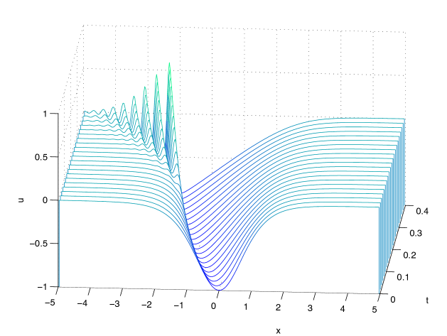
Figure 1. Solution to the KdV equation for the initial data $u_{0}(x)=-\mbox{sech}^{2}x$ and $\epsilon=10^{-1}$.

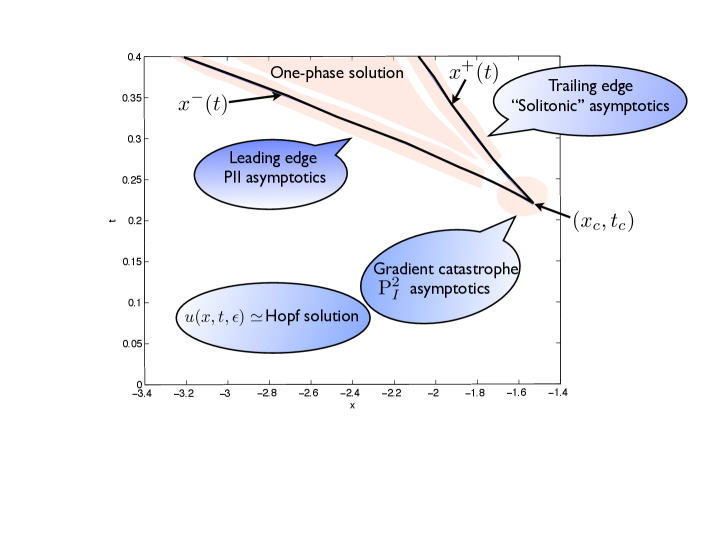
Figure 2. Whitham zone for the KdV equation for the initial data $u_{0}(x)=-\mbox{sech}^{2}x$. The shadow regions indicate the various asymptotic approximations in a neighbourhood of the Whitham zone.

Inside this cusp-shaped region, the exact one-phase solution to the KdV equation in terms of elliptic functions gives an asymptotic description of the oscillations, but on an elliptic surface where the branch points depend on $x$ and $t$ via the Whitham modulation equations as was proved by Lax and Levermore and Venakides [50, 59]. This averaging procedure works well inside the Whitham zone, but has to be amended near the boundaries of the zone as was found numerically in [39]. Near the point of gradient catastrophe $(x_{c},t_{c})$ , Dubrovin [28] conjectured that for a large class of equations containing KdV, the corresponding solution is asymptotically given in terms of a special solution of the second equation in the Painlevé I hierarchy that we will call ${\rm P}_{I}^{2}$ equation. This was tested numerically in [41] and proven for KdV in [15]. Near the leading edge a multiscale expansion was presented for the oscillations in terms of a particular solution of the Painlevé II equation in [40]. The validity of such an expansion has been proved rigorously in [16]. Near the trailing edge [17] gave an asymptotic solution in terms of a series of pulses of the shape of KdV solitons (see Fig 2).

It is remarkable that the KdV solutions can be approximated by Painlevé equations in the critical regimes described above. Those Painlevé equations have appeared in many branches of pure and applied mathematics during the past decades, for an overview we refer to [35].

The universal critical behaviour of KdV solutions should be seen in relation to the known universality results in random matrix theory. For large unitary random matrix ensembles, local eigenvalue statistics turn out to be, to some extent, independent of the choice of the ensemble and independent of the reference point chosen [25, 27]. Critical break-up times occur when the eigenvalues move from a one-cut regime to a multi-cut regime. These transitions take place in the presence of singular points, of which three different types are distinguished [27]. Such singular points have the same singularity type which appears in the small dispersion limit of KdV. Singular interior points [34, 32, 6, 19, 20] show remarkable similarities with the leading edge of the oscillatory region for the KdV equation. The second possibility, which is related to the trailing edge for KdV, is that an interval in the spectrum shrinks and disappears afterwards. This case is also referred to as birth of a cut in unitary random matrix ensembles, [5, 14, 52, 33]. The point of gradient catastrophe, i.e. the break-up point where the oscillations set in is comparable to a singular edge point in unitary random matrix ensembles. It was conjectured by Bowick and Brézin, and by Brézin, Marinari, and Parisi [9, 10] that local eigenvalue statistics in this regime should be given in terms of the Painlevé I hierarchy. In [22], it was proven that indeed double scaling limits of the local eigenvalue correlation kernel are given in terms of the Lax pair for the $P_{I}^{2}$ equation.

In this paper we implement numerically all known asymptotic approximations to the solution $u(x,t,\epsilon)$ of the KdV equation as $\epsilon\rightarrow 0$ and test them quantitatively for a concrete example. With respect to previous works, the numerical methods are overall improved which allows to study a wider range of values for the small dispersion parameter $\epsilon$. The asymptotic formulae for the trailing edge are implemented for the first time as well as the terms of order $\epsilon^{4/7}$ at the breakup point. We also address numerically the matching of different approximations.

The paper is organized as follows: In sect. 2 we collect various asymptotic formulae for KdV solutions in the small dispersion limit. In sect. 3 we give a brief overview of the used numerical methods. In sect. 4 we study numerically the asymptotic description given by the one-phase KdV and the Hopf solution. At the leading edge, the multiscale solution in terms of a special solution to the Painlevé II equation is studied in sect. 5. In sect. 6 the same is done for the asymptotic solution at the trailing edge, and in sect. 7 for the point of gradient catastrophe. In sect. 8 we add some concluding remarks and an outlook on the connection formulae for the various asymptotic regimes.

2. Asymptotic descriptions of the small dispersion limit

In this section we summarize various asymptotic descriptions of the dispersive shocks which will be implemented numerically in the following.

2.1. One-phase solution in the Whitham zone

Inside the cusp-shaped region in Fig. 2 for $t$ slightly bigger than $t_{c}$, the KdV solution $u(x,t,\epsilon)$ can be approximated for small $\epsilon$, by the exact $1$-phase solution of KdV, where the branch points of the elliptic surface depends on $x$ and $t$ through Whitham equations. The one-phase solution of KdV can be written in terms of the Jacobi elliptic theta function and the complete elliptic integrals of the first and second kind $E(s)$ and $K(s)$ [50, 26, 43]:

(2.1) $$u(x,t,\epsilon)\simeq\beta_{1}+\beta_{2}+\beta_{3}+2\alpha+2\epsilon^{2}\frac{\partial^{2}}{\partial x^{2}}\log\vartheta(\Omega(x,t);\mathcal{T}),$$

where $\beta_{1}>\beta_{2}>\beta_{3}$, $\Omega$, $\alpha$, and $\mathcal{T}$ have the form

(2.2) $$\Omega(x,t)=\dfrac{\sqrt{\beta_{1}-\beta_{3}}}{2\epsilon K(s)}[x-2t(\beta_{1}+\beta_{2}+\beta_{3})-q],$$

(2.3) $$\alpha(s)=-\beta_{1}+(\beta_{1}-\beta_{3})\frac{E(s)}{K(s)},\;\;\mathcal{T}=i\dfrac{K^{\prime}(s)}{K(s)},\;\;s^{2}=\frac{\beta_{2}-\beta_{3}}{\beta_{1}-\beta_{3}}.$$

Note that $K^{\prime}(s)=K(\sqrt{1-s^{2}})$, and $\vartheta$ is defined by the Fourier series

$$\vartheta(z;\mathcal{T})=\sum_{n\in\mathbb{Z}}e^{\pi in^{2}\mathcal{T}+2\pi inz}.$$

The formula for $q$ in the phase $\Omega$ in (2.2) is equal to [40, 26]

(2.4) $$q(\beta_{1},\beta_{2},\beta_{3})=\frac{1}{2\sqrt{2}\pi}\int_{-1}^{1}\int_{-1}^{1}d\mu d\nu\frac{f_{L}(\frac{1+\mu}{2}(\frac{1+\nu}{2}\beta_{1}+\frac{1-\nu}{2}\beta_{2})+\frac{1-\mu}{2}\beta_{3})}{\sqrt{1-\mu}\sqrt{1-\nu^{2}}},$$

where $f_{L}(y)$ is the inverse function of the decreasing part of the initial data $u_{0}$. The formula (2.4) for $q$ is valid as long as $\beta_{3}$ does not reach the minimum value of the initial data $u_{0}$. When $\beta_{3}$ reaches and goes beyond the negative hump it is also necessary to take into account the increasing part of the initial data $f_{R}$, [39], [56]

(2.5) $$q(\beta_{1},\beta_{2},\beta_{3})=\frac{1}{2\pi}\int_{\beta_{2}}^{\beta_{1}}\dfrac{d\lambda\left(\displaystyle\int_{\beta_{3}}^{-1}\frac{d\xi f_{R}(\xi)}{\sqrt{\lambda-\xi}}+\displaystyle\int_{-1}^{\lambda}\frac{d\xi f_{L}(\xi)}{\sqrt{\lambda-\xi}}\right)}{\sqrt{(\beta_{1}-\lambda)(\lambda-\beta_{2})(\lambda-\beta_{3})}}.$$

Remark 2.1.

In the formula (2.1) the term $\beta_{1}+\beta_{2}+\beta_{3}+2\alpha$ is the weak limit of $u(x,t,\epsilon)$ as $\epsilon\rightarrow 0$ [50] and the term containing the $\theta$-function describes the oscillations [26, 59]. The error term in the asymptotic expansion (2.1) should be of order $O(\epsilon)$.

Formula (2.1) can be written also in terms of the Jacobi elliptic function dn in the form

(2.6) $$u(x,t,\epsilon)\simeq\beta_{2}+\beta_{3}-\beta_{1}+2(\beta_{1}-\beta_{3})\mbox{dn}^{2}(2K(s)\Omega+K(s)).$$

For constant values of $\beta_{1}>\beta_{2}>\beta_{3}$, the right hand side of (2.6) is an exact solution of KdV. However in the description of the leading order asymptotics of $u(x,t,\epsilon)$ as $\epsilon\rightarrow 0$, the numbers $\beta_{1}>\beta_{2}>\beta_{3}$ depend on $x$ and $t$ and evolve according to the Whitham equations [60]

(2.7) $$\dfrac{\partial}{\partial t}\beta_{i}+v_{i}\dfrac{\partial}{\partial x}\beta_{i}=0,\quad v_{i}=4\frac{\prod_{k\neq i}(\beta_{i}-\beta_{k})}{\beta_{i}+\alpha}+2(\beta_{1}+\beta_{2}+\beta_{3}),\;\;\;i=1,2,3,$$

with $\alpha$ as in (2.3).

The Whitham equations (2.7) can be integrated through the so-called hodograph transform, which generalizes the method of characteristics, and which gives the solution in the implicit form [58]

(2.8) $$x=v_{i}t+w_{i},\quad i=1,2,3,$$

where the $v_{i}$ are defined in (2.7), and where $w_{i}=w_{i}(\beta_{1},\beta_{2},\beta_{3})$ for $i=1,2,3$ is obtained from an algebro-geometric procedure by the formula [55]

(2.9) $$w_{i}=\frac{1}{2}\left(v_{i}-2\sum_{k=1}^{3}\beta_{k}\right)\frac{\partial q}{\partial\beta_{i}}+q,\quad i=1,2,3,$$

with $q$ defined in (2.4) or (2.5). Solvability of (2.8) for initial data with a single hump was proved in [56].

Near the boundary of the oscillatory cusp-shaped region, neither the Hopf solution (1.3) nor the one-phase solution (2.1) gives a satisfactory description of the KdV solution $u(x,t,\epsilon)$ as $\epsilon\rightarrow 0$. Three different transitional regimes can be distinguished: (1) the cusp point where the gradient catastrophe for the Hopf equation takes place and where $\beta_{1}=\beta_{2}=\beta_{3}=u_{c}$, (2) the leading edge of the oscillatory zone where $\beta_{2}=\beta_{3}$, and (3) the trailing edge of the oscillatory zone where $\beta_{1}=\beta_{2}$. We will illustrate in the next subsections that in the above three cases

$$u(x,t,\epsilon)=\left\{\begin{array}[]{lll}u(x_{c},t_{c})+O(\epsilon^{\frac{2}{7}}),&\mbox{near the point of gradient catastrophe $(x_{c},t_{c})$ },&\\ u(x^{-}(t),t)+O(\epsilon^{\frac{1}{3}}),&\mbox{near the leading edge},&\\ u(x^{+}(t),t)+O(1),&\mbox{near the trailing edge},&\end{array}\right.$$

where $u(x,t)$ is the solution of the Hopf equation and $x^{\pm}(t)$ are the boundaries of the Whitham zone. The sub-leading terms are described respectively by a ${\rm P_{I}^{2}}$ transcendent, a ${\rm P_{II}}$ transcendent, and a train of solitons. Clearly the above asymptotic expansions are not uniform in $\epsilon$. Connections formula need to be developed.

2.2. Point of gradient catastrophe

It was conjectured in [28] and proved afterwards in [15] that the KdV solution $u(x,t,\epsilon)$ as $\epsilon\rightarrow 0$ near the point of gradient catastrophe $(x_{c},t_{c})$ for the Hopf solution (1.3), is given in terms of a distinguished Painlevé transcendent, namely a special smooth solution $U(X,T)$ to the fourth order ODE

(2.11) $$X=6T\,U-\left[U^{3}+\dfrac{1}{2}U_{X}^{2}+U\,U_{XX}+\frac{1}{10}U_{XXXX}\right].$$

This ODE is the second member of the Painlevé I hierarchy, and we refer to it as the ${\rm P_{I}^{2}}$ equation. The relevant solution is real and has the asymptotic behavior

(2.12) $$U(X,T)=\mp(|X|)^{1/3}\mp 2T|X|^{-1/3}+\mathcal{O}(|X|^{-1}),\qquad\mbox{as $X\to\pm\infty$,}$$

for any fixed $T\in\mathbb{R}$, and has no poles for real values of $X$ and $T$ [21, 28]. It is remarkable that $U(X,T)$ is an exact solution to the KdV equation

(2.13) $$U_{T}+6UU_{X}+U_{XXX}=0.$$

In a double scaling limit where $\epsilon\to 0$ and simultaneously $x$ and $t$ approach the point and the time of gradient catastrophe $x_{c}$ and $t_{c}$ in such a way that the limits

$$\lim_{\begin{matrix}\epsilon\rightarrow 0\\ x-6u_{c}t\rightarrow x_{c}-6u_{c}t_{c}\end{matrix}}\left[\dfrac{x-x_{c}-6u_{c}(t-t_{c})}{\epsilon^{\frac{6}{7}}}\right],\quad\lim_{\begin{matrix}\epsilon\rightarrow 0\\ t\rightarrow t_{c}\end{matrix}}\left[\dfrac{(t-t_{c})}{\epsilon^{\frac{4}{7}}}\right],\;\;\;u_{c}=u(x_{c},t_{c})$$

exist and are bounded, the KdV solution has an expansion of the following form [15]. Let

(2.14) $$X=\dfrac{x-x_{c}-6u_{c}(t-t_{c})}{(k)^{1/7}\epsilon^{\frac{6}{7}}},\quad T=\dfrac{(t-t_{c})}{(k)^{3/7}\epsilon^{\frac{4}{7}}}$$

with

(2.15) $$k=-f^{\prime\prime\prime}_{L}(u_{c})/6$$

and $f_{L}(u)$ the inverse of the decreasing part of the initial data. Then the solution of KdV is approximated by

(2.16) $$\begin{split}u(x,t,\epsilon)&=u_{c}+\left(\frac{\epsilon}{k}\right)^{2/7}U(X,T)-\left(\frac{\epsilon}{k}\right)^{4/7}\dfrac{f_{L}^{(IV)}(u_{c})}{63f_{L}^{\prime\prime\prime}(u_{c})}\times\\ &\left[QU_{X}+2U_{XX}+4U^{2}+15T-90T^{2}U_{X}-3XUU_{X}-\dfrac{1}{2}XU_{XXX}\right]+O(\epsilon^{\frac{5}{7}})\end{split}$$

and $Q(X,T)$ is the integral of $U(X,T)$,

$$Q=\dfrac{1}{10}U_{X}U_{XXX}-\dfrac{1}{20}U_{XX}^{2}+XU-3TU^{2}+\dfrac{1}{4}U^{4}+\dfrac{1}{2}UU_{X}^{2},\;\;Q_{X}=U.$$

The correction term of order $\epsilon^{\frac{2}{7}}$ was rigorously derived using steepest descent analysis for the Riemann-Hilbert problem for KdV in [15]. Such an approximation was already discovered for the Gurevich-Pitaevskii solution of KdV in [54]. The correction of order $\epsilon^{4/7}$ was derived in [18].

2.3. Leading edge

Near the leading edge at the left of the zone where the oscillations become small, a multiscale analysis and numerical results [40] showed that the envelope of the oscillations is asymptotically described by a particular solution to the second Painlevé equation (${\rm P}_{II}$)

(2.17) $$q^{\prime\prime}(s)=sq+2q^{3}(s).$$

The special solution we are interested in, is the Hastings-McLeod solution [44] which is uniquely determined by the boundary conditions

(2.18) $$q(s)=\sqrt{-s/2}(1+o(1)), s\to-\infty$$ as ,

(2.19) $$q(s)=\mbox{Ai}(s)(1+o(1)), s\to+\infty$$ as ,

where $\mbox{Ai}(s)$ is the Airy function. Although any nonzero Painlevé II solution has an infinite number of poles in the complex plane, it is known [44] that the Hastings-McLeod solution $q(s)$ is smooth for all real values of $s$.

The leading edge corresponds to the Whitham equations in the confluent case where

$$\beta_{3}(x,t)=\beta_{2}(x,t)=v(t),\qquad\beta_{1}(t)=u(t),$$

see also (2.1). There exists a time $\tilde{t}>t_{c}$ such that for $t_{c}<t<\tilde{t}$, the leading edge $x^{-}(t)$ is determined uniquely by the system of equations [55, 42]

(2.20) $$x^{-}(t)=6tu(t)+f_{L}(u(t)),$$

(2.21) $$6t+\theta(v(t);u(t))=0,$$

(2.22) $$\partial_{v}\theta(v(t);u(t))=0,$$

with $u(t)>v(t)$ and with

(2.23) $$\theta(v;u)=\theta(v;u)=\dfrac{1}{2\sqrt{2}}\int_{-1}^{1}f^{\prime}_{L}\left(\frac{1+m}{2}v+\frac{1-m}{2}u\right)\dfrac{dm}{\sqrt{1-m}}.$$

Furthermore $x^{-}(t)$, $u(t)$, and $v(t)$ are smooth functions of $t$. Throughout the rest of the subsection, whenever we refer to $u$, we mean by this the solution of the system (2.20)-(2.22) for a given time $t_{c}<t<\tilde{t}$, while we denote the solution of the KdV equation as $u(x,t,\epsilon)$ and the solution of the Hopf equation as $u(x,t)$.

The behaviour of the solution of KdV near the leading edge as $\epsilon\rightarrow 0$ is described as follows. Take a double scaling limit where $\epsilon\to 0$ and at the same time $x\to x^{-}(t)$ in such a way that

(2.24) $$\lim_{\begin{matrix}\epsilon\rightarrow 0\\ x\rightarrow x^{-}(t)\end{matrix}}\left[\dfrac{x-x^{-}(t)}{\epsilon^{2/3}}\right]$$

remains bounded. In this double scaling limit, the solution $u(x,t,\epsilon)$ of the KdV equation (1.1) with initial data $u_{0}$ has the asymptotic expansion [16]

(2.25) $$u(x,t,\epsilon)=u-\dfrac{4\epsilon^{1/3}}{c^{1/3}}q\left(s(x,t,\epsilon)\right)\cos\left(\frac{\Theta(x,t)}{\epsilon}+\epsilon^{1/3}\Theta_{1}(x,t,\epsilon)\right)\\ +\frac{x-x^{-}}{6t+f^{\prime}_{L}(u)}-\dfrac{4\epsilon^{2/3}}{c^{2/3}(u-v)}q\left(s(x,t,\epsilon)\right)^{2}\sin^{2}\left(\frac{\Theta(x,t)}{\epsilon}\right)+O(\epsilon).$$

Here $x^{-}$ and $v<u$ (each of them depending on $t$) solve the system (2.20), and the phase $\Theta(x,t)$ is given by

(2.26) $$\Theta(x,t)=2\sqrt{u-v}(x-x^{-})+2\int_{v}^{u}(f_{L}^{\prime}(\xi)+6t)\sqrt{\xi-v}d\xi.$$

Furthermore

(2.27) $$c=-\sqrt{u-v}\dfrac{\partial^{2}}{\partial v^{2}}\theta(v;u)>0,\qquad s(x,t,\epsilon)=-\frac{x-x^{-}}{c^{1/3}\sqrt{u-v}\,\epsilon^{2/3}},$$

with $\theta$ defined by (2.23), and $q$ is the Hastings-McLeod solution to the Painlevé II equation. The correction to the phase $\Theta_{1}(x,t,\epsilon)$ takes the form

(2.28) $$\Theta_{1}(x,t,\epsilon)=\frac{1}{c^{1/3}}\left[\left(\frac{q^{\prime}}{q}+p\right)\frac{\partial^{3}_{v^{3}}\theta(v;u)}{6\partial^{2}_{v^{2}}\theta(v;u)}-\frac{5p+\frac{q^{\prime}}{q}}{4(u-v)}\right.\\ \left.+\dfrac{s(x,t,\epsilon)^{2}}{4}\left(\frac{\partial^{3}_{v^{3}}\theta(v;u)}{3\partial^{2}_{v^{2}}\theta(v;u)}-\frac{3}{2(u-v)}+\dfrac{2c\sqrt{u-v}}{6t+f^{\prime}_{L}(u)}\right)\right],$$

where we used the notations

$$q=q(s),\qquad q^{\prime}=q^{\prime}(s),\qquad p=p(s)=-q^{4}(s)-sq^{2}(s)+q^{\prime}(s)^{2},$$

with $s=s(x,t,\epsilon)$ and $p^{\prime}(s)=-q^{2}$.

Remark 2.2.

Note that the leading order term in the expansion (2.25) of $u(x,t,\epsilon)$ is given by $u(t)$ the solution of the Hopf equation at the leading edge. The second term in (2.25) is of order $\epsilon^{1/3}$, while the remaining terms are of order $\epsilon^{2/3}$. From the $\mathcal{O}(\epsilon^{1/3})$-term, we observe that $u(x,t,\epsilon)$ develops oscillations of wavelength $\mathcal{O}(\epsilon)$ at the leading edge, the envelope of the oscillations is proportional to the Hastings-McLeod solution $q$. If we let $(x-x^{-}(t))/\epsilon^{\frac{2}{3}}\to-\infty$ (so that $x$ lies to the left of the leading edge), the terms with the oscillations disappear due to the exponential decay of $q$, see (2.19). We are then left with only two terms in (2.25), which are the first two terms in the Taylor series of the Hopf solution $u(x,t)$ near $x^{-}$.

Remark 2.3.

The formula (2.25) can be obtained from a multiple scale analysis [40] from (2.1), letting

$$\beta_{3}(x,t)=v(t)-\dfrac{2\epsilon^{1/3}}{c^{1/3}}q\left(s(x,t,\epsilon)\right),\quad\beta_{2}(x,t)=v(t)+\dfrac{2\epsilon^{1/3}}{c^{1/3}}q\left(s(x,t,\epsilon)\right),$$

$$\qquad\beta_{1}(t)=u(t)+\frac{x-x^{-}}{6t+f^{\prime}_{L}(u)}.$$

2.4. Trailing edge

The trailing edge $x^{+}(t)$ of the oscillatory interval is uniquely determined by the confluent form $\beta_{1}=\beta_{2}=v$ and $\beta_{3}=u$, $v>u$, of the equations (2.8), namely [55, 42]

(2.29) $$x^{+}(t)=6tu(t)+f_{L}(u(t)),$$

(2.30) $$6t+\theta(v(t);u(t))=0,$$

(2.31) $$\int_{u(t)}^{v(t)}(6t+\theta(\lambda;u(t)))\sqrt{\lambda-u(t)}d\lambda=0,$$

where $\theta(v;u)$ has been defined in (2.23).

Let $x^{+}=x^{+}(t)$, $u=u(t)$, and $v=v(t)$ solve the system (2.29)-(2.31), and let us take a double scaling limit where $\epsilon\to 0$ simultaneously with $x\to x^{+}(t)$ in such a way that

$$y:=2\sqrt{v-u}\,\frac{x-x^{+}}{\epsilon\ln\epsilon}$$

remains bounded: there exists a real $M>0$ such that $|y|<M$. Then there exists $\tilde{t}>t_{c}$ such that for $t_{c}<t<\tilde{t}$, we have the following expansion for the KdV solution $u(x,t,\epsilon)$ in the double scaling limit [17],

(2.33) $$u\left(x,t,\epsilon\right)=u+2(v-u)\sum_{j=0}^{\lceil M\rceil}{\rm sech}^{2}(X_{j})+\mathcal{O}(\epsilon\ln^{2}\epsilon),$$

where $\lceil M\rceil$ is the smallest integer $\geq M$,

(2.34) $$\begin{split}&X_{j}=\frac{1}{2}(\frac{1}{2}-y+j)\ln\epsilon-\ln(\sqrt{2\pi}h_{j})-(j+\frac{1}{2})\log\gamma,\\ &h_{j}=\dfrac{2^{\frac{j}{2}}}{\pi^{\frac{1}{4}}\sqrt{j!}},\quad\gamma=4(v-u)^{\frac{5}{4}}\sqrt{-\partial_{v}\theta(v;u)},\end{split}$$

and $\theta$ is given by (2.23). Observe that $h_{j}$ are the normalization constants of the Hermite polynomials.

Remark 2.4.

Observe that each term in the sum of (2.33) generates a pulse with amplitude $2(v-u)$ for $y$ near a half positive integer which can be seen as a soliton. Indeed the term ${\rm sech}^{2}(X_{j})$ is of the order $O(1)$ for $y=j+1/2$. For $y=j$ or $j+1$, it already decreased to order $O(\epsilon^{\frac{1}{2}})$. For $y=j-\frac{1}{2}$ or $j+\frac{3}{2}$, the contribution of ${\rm sech}^{2}(X_{j})$ is absorbed by the error term $O(\epsilon\ln^{2}\epsilon)$. Clearly, since $j$ is nonnegative, the solitons appear only for $y$ positive, that is for $x<x^{+}$, namely inside the Whitham zone.

Remark 2.5.

The phase defined in (2.2) satisfies the formal limit

$$2K(s)\Omega|_{\beta_{1}\simeq\beta_{2}}=\dfrac{x-x^{+}}{\epsilon}\sqrt{v-u}+O((\beta_{1}-\beta_{2})^{2}),$$

and from the Whitham solution (2.8) one obtains in the limit $\beta_{1}\rightarrow\beta_{2}$

$$x-x^{+}(t)\simeq-\dfrac{1}{4}\partial_{v}\theta(v;u)\left(\dfrac{\beta_{1}-\beta_{2}}{2}\right)^{2}\log\left(\dfrac{\beta_{1}-\beta_{2}}{2}\right)^{2}.$$

The Jacobi elliptic function $\mbox{dn}\rightarrow{\rm sech}$ as the modulus $s\rightarrow 1$ and

$$K(s)\simeq\dfrac{1}{2}\log\left[\dfrac{8}{1-s}\right],\quad\mbox{as}\;\;s\rightarrow 1.$$

Therefore the formal limit of the solution (2.6) in terms of elliptic functions as $s\rightarrow 1$, $\beta_{1},\beta_{2}\rightarrow v$, $\beta_{3}\rightarrow u$, gives

(2.35) $$u(x,t,\epsilon)\simeq u+2(v-u)\,{\rm sech}^{2}\left[\dfrac{x-x^{+}}{\epsilon}\sqrt{v-u}+(j+\dfrac{1}{2})\log\left[\dfrac{8}{1-s}\right]\right],$$

for any positive integer $j$, due to the periodicity of the elliptic function dn. Choosing

$$\left(\dfrac{\beta_{1}-\beta_{2}}{2}\right)^{2}=\dfrac{4\epsilon}{\partial_{v}\theta(v,u)\sqrt{v-u}}$$

and inserting it in (2.35) one can partially reproduce the formula (2.33) in the sense that all the terms in the phase $X_{j}$ defined in (LABEL:Xj) can be reproduced except the one containing the normalization constants of the Hemite polynomials $h_{j}$. We would like to remark that the formal limit (2.35) has appeared several times in the literature, but such limit does not describe the small dispersion solution of KdV near the trailing edge, since the limiting value of the phase (2.2) does not give the right result.

3. Numerical Methods

The numerical task in treating the small dispersion limit of KdV and various asymptotic formulas consists in solving the KdV equation itself, certain ODEs of Painlevé type for a given asymptotic behavior, and of the Whitham equations for which the implicit solution (2.7) exists. We will summarize in this section how these different tasks are solved numerically, and how we control the numerical accuracy.

3.1. KdV solution

Since critical phenomena are generally believed to be independent of the chosen boundary conditions, we study a periodic setting in the following. This also includes rapidly decreasing functions which can be periodically continued as smooth functions within the finite numerical precision. This allows to approximate the spatial dependence via truncated Fourier series which leads for the studied equations to large stiff systems of ordinary differential equations (ODEs), see below. The use of Fourier methods not only gives spectral accuracy in the spatial coordinates (the numerical error in approximating smooth functions decreases faster than any power of the number $N$ of Fourier modes), but also minimizes the introduction of numerical dissipation which is important in the study of the purely dispersive effects we are interested in here. In Fourier space, equation (1.1) has the form

(3.1) $$v_{t}=\mathbf{L}v+\mathbf{N}(v,t),$$

where $v$ denotes the (discrete) Fourier transform of $u$, and where $\mathbf{L}$ and $\mathbf{N}$ denote linear and nonlinear operators, respectively. The resulting system of ODEs consists in this case of stiff equations where the stiffness is related to the linear part $\mathbf{L}$ (it is a consequence of the distribution of the eigenvalues of $\mathbf{L}$), whereas the nonlinear part contains only low order derivatives. In the small dispersion limit, this stiffness is still present despite the small term $\epsilon^{2}$ in $\mathbf{L}$. This is due to the fact that the smaller $\epsilon$ is, the higher wavenumbers are needed to resolve the rapid oscillations.

Loosely speaking a stiff system is a system for which explicit numerical schemes as explicit Runge-Kutta methods are inefficient, since prohibitively small time steps have to be chosen to control exponentially growing terms. The standard remedy for this is to use stable implicit schemes, which require, however, the iterative solution of a system of nonlinear equations at each time step which is computationally expensive. In addition the iteration often introduces numerical errors in the Fourier coefficients. Thus we used in [39] an integrating factor method, where the linear stiff part is explicitly integrated. This can be conveniently done here since the operator $\mathbf{L}$ corresponding to the third derivative with respect to $x$ is diagonal in Fourier space. As was shown in [45], integrating factor methods can suffer from order reductions, which means that the actual decrease of the numerical error with the numerical resolution is much lower than the classical order of the used method. This was confirmed for the small dispersion limit of KdV in [48]. There it was also shown that exponential time differencing (ETD) schemes are very efficient for KdV. ETD schemes were developed originally by Certaine [12] in the 60s, see [46] for a comprehensive review. The basic idea is to use equidistant time steps $h$ and to integrate equation (3.1) exactly between the time steps $t_{n}$ and $t_{n+1}$ with respect to $t$. With $v(t_{n})=v_{n}$ and $v(t_{n+1})=v_{n+1}$, we get

$$v_{n+1}=e^{\mathbf{L}h}v_{n}+\int_{0}^{h}e^{\mathbf{L}(h-\tau)}\mathbf{N}(v(t_{n}+\tau),t_{n}+\tau)d\tau.$$

The integral will be computed in an approximate way for which different schemes exist. We use here a Runge-Kutta method of classical order 4 due to Cox-Matthews [24]. As in [1] for the Camassa-Holm equation, this approach could be amended by identifying two regimes $t\in[0,t_{1}]$ and $t\in[t_{1},t_{end}]$ with $t_{1}\ll t_{c}$. A much larger time step can be used in the first regime than in the second where the rapid modulated oscillations appear. We do not use this approach here since it was not necessary for the considered values of $\epsilon$.

The accuracy of the numerical solution is controlled via the numerically computed conserved energy of the solution

(3.2) $$E[u]=\int_{\mathbb{T}}(2u^{3}-\epsilon^{2}u_{x}^{2})dx,$$

which is an exactly conserved quantity for KdV. Numerically the energy $E$ will be a function of time. We define $\Delta E:=|(E(t)-E(0))/E(0)|$. It was shown in [48] that this quantity can be used as an indicator of the numerical accuracy if sufficient resolution in space is provided. The quantity $\Delta E$ typically overestimates the precision by two orders of magnitude. Since the numerical error has to be clearly smaller than the difference between KdV solution and the asymptotic descriptions we want to test (which give at best descriptions of order $\epsilon$) we are interested in a numerical value clearly below the smallest considered value of $\epsilon$. To ensure this we will always ensure that the modulus of the Fourier coefficients of the final state decreases well below $10^{-5}$ (thus providing the needed resolution), and that the quantity $\Delta E$ is smaller than $10^{-6}$ (in general it is of the order of machine precision, i.e. $10^{-14}$).

We consider in the following always the example $u_{0}=-\mbox{sech}^{2}x$ and values of

$$\epsilon=10^{-1},10^{-1.25},\ldots 10^{-3.5}.$$

For the smallest values of $\epsilon$, we use $N=2^{19}$ Fourier modes and $N_{t}=4*10^{5}$ time steps; for larger values of $\epsilon$ between $2^{15}$ and $2^{17}$ Fourier modes, and between $10^{4}$ to $10^{5}$ time steps. The oscillatory zone for $\epsilon=10^{-3.5}$ can be seen in Fig. 3. The Fourier coefficients for this solution are shown in Fig. 4.

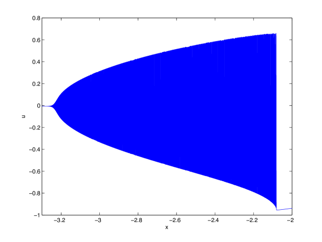
Figure 3. The oscillatory zone in the solution to the KdV equation for the initial data $u_{0}(x)=-\mbox{sech}^{2}x$ and $\epsilon=10^{-3.5}$ for $t=0.4$. The oscillations are so rapid, that they are graphically difficult to represent though they are numerically well resolved.

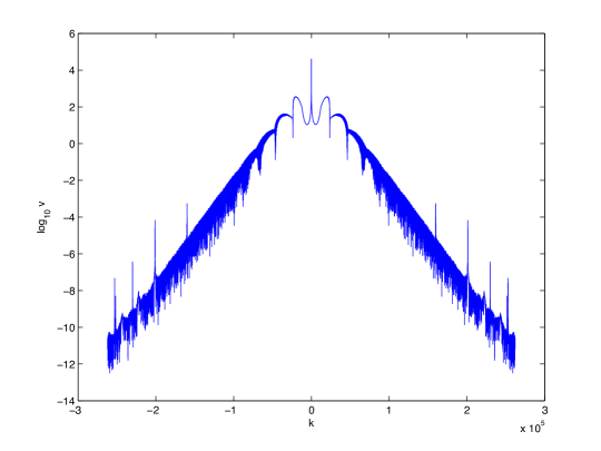
Figure 4. Fourier coefficients for the solution in Fig. 3.

3.2. Numerical solution of the Whitham equations and of the Hopf equation

The Whitham equations (2.7) are solved for given initial data by inverting the hodograph transform (2.8) to obtain $\beta_{1}>\beta_{2}>\beta_{3}$ as a function of $x$ and $t$, and similarly for the implicit solution of the Hopf equation (1.3). Since the hodograph transform becomes degenerate at the leading and trailing edge we solve the system (2.20)–(2.22) and (2.29)–(2.31) instead of (2.8) to avoid convergence problems.

These equations are of the form

(3.3) $$S_{i}(\{y_{i}\},x,t)=0,\quad i=1,\ldots,M,$$

where the $S_{i}$ denote some given real function of the $y_{i}$ and $x$, $t$. The task is to determine the $y_{i}$ in dependence of $x$ and $t$. To this end we determine the $y_{i}$ for given $x$ and $t$ as the zeros of the function $S:=\sum_{i=1}^{M}S_{i}^{2}$. This is done numerically by using the algorithm of [49] which is implemented as the function fminsearch in Matlab. The algorithm provides an iterative approach which converges in our case rapidly if the starting values are close enough to the solution (see below how the starting values are chosen). We calculate the zeros to the order of machine precision.

For a given $t>t_{c}$, we always first solve the system (2.20)–(2.22) to obtain the leading edge coordinate $x^{-}(t)$ and

$$\beta_{1}^{-}(t)>\beta^{-}_{2}(t)=\beta^{-}_{3}(t).$$

Similarly we solve the equations (2.33) for $x^{+}$ and $\beta_{1}^{+}=\beta_{2}^{+}$ and $\beta_{3}^{+}$ which fixes the interval $[x^{-},x^{+}]$. This interval is subdivided into a number of points $x_{n}$, $n=1,\ldots,N_{x}$. In contrast to [39], we choose the $x_{n}$ to be related to Chebyshev collocation points $l_{j}=\cos(j\pi/N_{c})$, $j=0,1\ldots,N_{c}$, to allow for better interpolation formulas. Since the polynomial interpolation we will use works best for smooth functions, we use the analytic knowledge that $\beta_{2}\sim\beta_{3}\sim\sqrt{x-x^{-}(t)}$ for $x\sim x^{-}(t)$, and similarly $\beta_{1}\sim\beta_{2}\sim\sqrt{x^{+}(t)-x}$ for $x\sim x^{+}(t)$. Thus we put for $j=0,\ldots,N_{c}$

$$x_{j}=x^{-}(t)+\frac{x^{+}(t)-x^{-}(t)}{2}\frac{(1+l_{j})^{2}}{4},\quad x\in[x^{-}(t),\frac{1}{2}(x^{-}(t)+x^{+}(t))]$$

and

$$x_{j}=x^{+}(t)-\frac{x^{+}(t)-x^{-}(t)}{2}\frac{(1-l_{j})^{2}}{4},\quad x\in[\frac{1}{2}(x^{-}(t)+x^{+}(t)),x^{+}(t)].$$

For given $x_{j}$ and $t$, the Whitham equations are solved as discussed in [39]. Thus the $\beta_{i}$ are sampled on Chebyshev collocation points which can be used to obtain an expansion of these functions in terms of Chebyshev polynomials, see for instance [36]. As for Fourier series, the order of magnitude of the modulus of the coefficient of the highest order polynomial gives for smooth functions an indication of the numerical resolution. For our example the Chebyshev coefficients decrease well below $10^{-6}$ with $N_{c}=64$ which is more than sufficient for our purposes. To obtain machine precision, the integrals in (2.8) would have to be computed as described in [39] with higher precision for $x$ close to the boundaries of the Whitham zone. The $\beta_{i}$ for the initial data $u_{0}=-\mbox{sech}^{2}x$ for $t=0.4$ can be seen in Fig. 5.

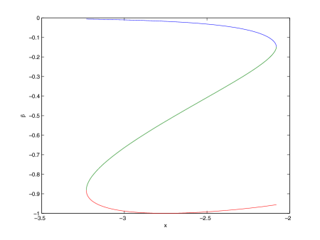
Figure 5. Solutions of the Whitham equations (2.8) for the initial data $u_{0}=-\mbox{sech}^{2}x$ for $t=0.4$.

At intermediate values of $x\in[x^{-}(t),x^{+}(t)]$, the $\beta_{i}$ are obtained from the values on the collocation points via numerically stable barycentric Lagrange interpolation, see [2], which is essentially an efficient implementation of the Lagrange polynomial for Chebyshev collocation points.

3.3. Painlevé transcendents

The asymptotic solutions near the breakup point and the leading edge are given by pole-free solutions with a given asymptotic behaviour for $x\to\pm\infty$ to the P${}^{2}_{I}$ equation and the Painlevé II equation respectively. A way to solve these equations is to give a series solution to the respective equation with the imposed asymptotics that is generally divergent. These divergent series are truncated at finite values of $x$, $x_{l}<x_{r}$ at the first term that is of the order of machine precision. The sum of this truncated series at these points is then used as boundary data, and similarly for derivatives at these points. Thus the problem is translated to a boundary value problem on the finite interval $[x_{l},x_{r}]$.

In [40] we used for the ${\rm P}_{I}^{2}$ solution a collocation method with cubic splines distributed as bvp4 with Matlab, in [41] for the Hastings-McLeod solution of ${\rm P}_{II}$ a Chebyshev collocation method with a fixed point iteration. Here we use again a Chebyshev collocation method for both equations. As for the Whitham equations above, the solution of the ODEs is sampled on Chebyshev collocation points $x_{j}$, $j=0,\ldots,N_{c}$ which can be related to an expansion of the solution in terms of Chebyshev polynomials. Since the derivative of a Chebyshev polynomial can be again expressed in terms of a linear combination of Chebyshev polynomials, the action of the derivative operator on the Hilbert space of Chebyshev polynomials is equivalent to the action of a matrix on this space. This leads to the well known Chebyshev differentiation matrices, see for instance [57]. Thus for the numerical solution, in an ODE of the form $F(u,\partial_{x}u,..)=0$, $u$ is replaced by the vector $u(x_{j})$, $j=0,\ldots,N_{c}$ and $\partial_{x}$ by the differentiation matrix. The ODE is in this setting replaced by $N_{c}+1$ algebraic equations. The boundary data are included via a so-called $\tau$-method: The equations for $j=0$ and for $j=N_{c}$ (for the fourth order equation $j=0,1,N_{c}-1,N_{c}$) are replaced by the boundary conditions. The resulting system of algebraic equations is solved with a standard Newton method. The convergence of the solutions is in general very fast. We always stop the Newton iteration when machine precision is reached. Again the highest Chebyshev coefficients are taken as an indication of sufficient resolution of the solutions (they have to reach machine precision). A similar approach had been used in [7] for the Hastings-McLeod solution. Solutions to the Painlevé II equation have been computed as the solution of a Riemann-Hilbert problem in [53]. Certain Painlevé transcendents can be expressed in terms of Fredholm determinants which can be computed with the methods of [8]. For the study of Painlevé solutions with poles in the complex plane, an approach based on Padé approximants has been presented in [37].

The Hastings-McLeod solution and the special solution to the ${\rm P}_{I}^{2}$ equation for various values of $t$ can be seen in Fig. 6.

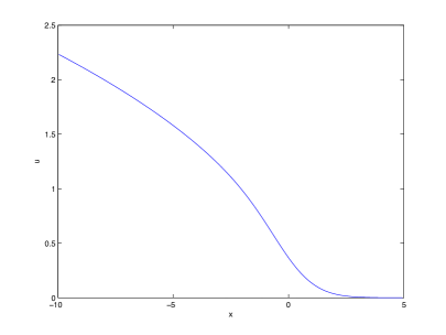
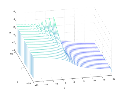
Figure 6. Hastings-McLeod solution of the Painlevé II equation on the left, and the special solution to the Painlevé I2 equation for several values of $t$ on the right.

4. Numerical solution of KdV, Whitham and Hopf equations

In this and the following sections, we will numerically solve the KdV equation (1.1) for the initial data $u_{0}(x)=-\mbox{sech}^{2}x$ for the values $\epsilon=10^{-1},10^{-1.25},\ldots,10^{-3.5}$, and compute the various asymptotic descriptions of the small dispersion limit from sect. 2. We will study the validity of these asymptotic descriptions in various regions of the $(x,t)$-plane. To obtain the $\epsilon$-dependence of a certain quantity $A$, we perform a linear regression analysis for the dependence of the logarithms, $\ln A=a\ln\epsilon+b$. This allows to obtain numerically the scaling of the difference between numerical and asymptotic solutions also for the cases where no analytic behavior is yet known. We first consider the asymptotic description based on the Hopf solution outside the Whitham zone and the one-phase KdV solution inside the zone with branch po of the elliptic surface given by the Whitham equations.

Outside the Whitham zone, the Hopf solution for the same initial data as the KdV solution gives an asymptotic description of the latter. Inside the Whitham zone, the one-phase KdV solution provides an asymptotic solution.

Before breakup:

For times much smaller than the critical time, we find that the $L_{\infty}$ norm of the difference between Hopf and KdV solutions decreases as $\epsilon^{2}$. More precisely we find by linear regression an exponent $a=1.9987$ with correlation coefficient $r=0.999995$ and standard deviation $a=0.0051$.

At breakup, $t=t_{c}$:

For times close to the breakup time, the Hopf solution develops a gradient catastrophe. The largest difference between Hopf and KdV solution can be found close to the breakup point. We determine the scaling of the $L_{\infty}$ norm of the difference between Hopf and KdV solutions on the whole interval of computation. We find that its scaling is compatible with $\epsilon^{2/7}$ as conjectured in [28] and proven in [15]. More precisely we find in a linear regression analysis $a=0.2929$ ($2/7=0.2857\ldots$) with a correlation coefficient $r=0.99996$ and standard deviation $a=0.0022$.

After breakup:

For times much greater than the critical time of the Hopf solution, we find that the asymptotic solution given by Hopf solution and the one-phase KdV solution via the Whitham equations gives a very good description of the KdV solution. Thus it is necessary to plot the difference between these solutions as done in Fig. 7

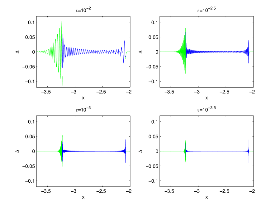
Figure 7. The blue line describes the difference between the numerical solution of the KdV equation and the asymptotic formula (2.1) for the initial data $u_{0}(x)=-1/\cosh^{2}x$ and for $t=0.4$. The green lines represent the difference between the numerical solution of the KdV equation and the Hopf solution (1.3).

It can be seen that this difference is not uniform in $x$, and that this applies also for the decrease with $\epsilon$. The approximation is very good close to the centre of the Whitham zone, but much worse at the edges. We define the interior part of the zone tentatively as the interval symmetric to the centre of half the length of the zone. The results do not depend on whether this zone is taken slightly smaller or bigger. We find that the $L_{\infty}$ norm of the difference of the numerical KdV solution and the one-phase KdV solution (2.1) decreases there roughly as $\epsilon$. More precisely we find in a linear regression analysis $a=0.98$ with a correlation coefficient $r=0.998$ and standard deviation $a=0.047$.

At the leading edge we find that the error is always biggest close to the boundary of the Whitham zone. In an interval symmetric to this boundary with the same length as the above interior zone, we find that the difference between KdV solution and asymptotic solutions via Hopf and the one-phase KdV solution (2.1) scale roughly as $\epsilon^{1/3}$. More precisely we find in a linear regression analysis $a=0.33$ with a correlation coefficient $r=0.999$ and standard deviation $a=0.012$.

The situation at the trailing edge is more complicated. It can be seen in Fig. 7 that the difference between the KdV solution and one-phase KdV solution (2.1) is almost constant (roughly 0.04) there. Notice that this error of order $\mathcal{O}(1)$ which is supposed to appear in a zone of width $\epsilon\ln\epsilon$ close to the trailing edge of the Whitham zone was not seen in [39] because of a lack of resolution. This is one of the reasons why we redid the computations with a considerably higher resolution. It can also be seen in Fig. 7 that the $\mathcal{O}(1)$ oscillation is moving closer and closer to the edge with smaller $\epsilon$ as expected. The difference between KdV and Hopf solutions close to the trailing edge decreases, however, roughly as $\sqrt{\epsilon}$. More precisely we find in a linear regression analysis $a=0.54$ with a correlation coefficient $r=0.997$ and standard deviation $a=0.03$.

5. Leading edge

In this section we study numerically the asymptotic formula (2.25) via the Hastings-McLeod solution which approximates the KdV solution at the leading edge as $\epsilon\rightarrow 0$. We will refer to this asymptotic solution as ${\rm P}_{II}$ asymptotics. We identify the zone, where the ${\rm P}_{II}$ asymptotics gives a better description of KdV than the Hopf (1.4) or the one-phase KdV solution (2.1) and study the $\epsilon$-dependence of the errors.

In Fig. 8 we show the KdV solution, the asymptotic solution via Whitham and Hopf and the ${\rm P}_{II}$- asymptotics near the leading edge of the Whitham zone. It can be seen that the one-phase KdV solution gives a very good description in the interior of the Whitham zone as discussed above, whereas the ${\rm P}_{II}$ asymptotics gives as expected a better description near the leading edge.

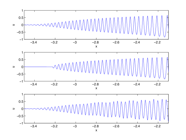
Figure 8. The figure shows in the upper part the numerical solution to the KdV equation for the initial datum $u_{0}=-\mbox{sech}^{2}x$ and $\epsilon=10^{-2}$ at $t=0.4$, in the middle the corresponding asymptotic solution in terms of Hopf and one-phase KdV solution, and in the lower part the ${\rm P}_{II}$ asymptotic solution (2.25).

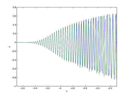
Figure 9. The numerical solution to the KdV equation for the initial datum $u_{0}=-\mbox{sech}^{2}x$ and $\epsilon=10^{-2}$ at $t=0.4$ in blue and the corresponding ${\rm P}_{II}$ asymptotic solution (2.25) in green.

In Fig. 9 the KdV solution and the ${\rm P}_{II}$ asymptotics are shown in one plot for $\epsilon=10^{-2}$. It can be seen that the agreement near the edge of the Whitham zone is so good that one has to study the difference of the solutions. The solution only gives locally an asymptotic description and is quickly out of phase for larger distances from the leading edge, whereas the amplitude is roughly of the right size.

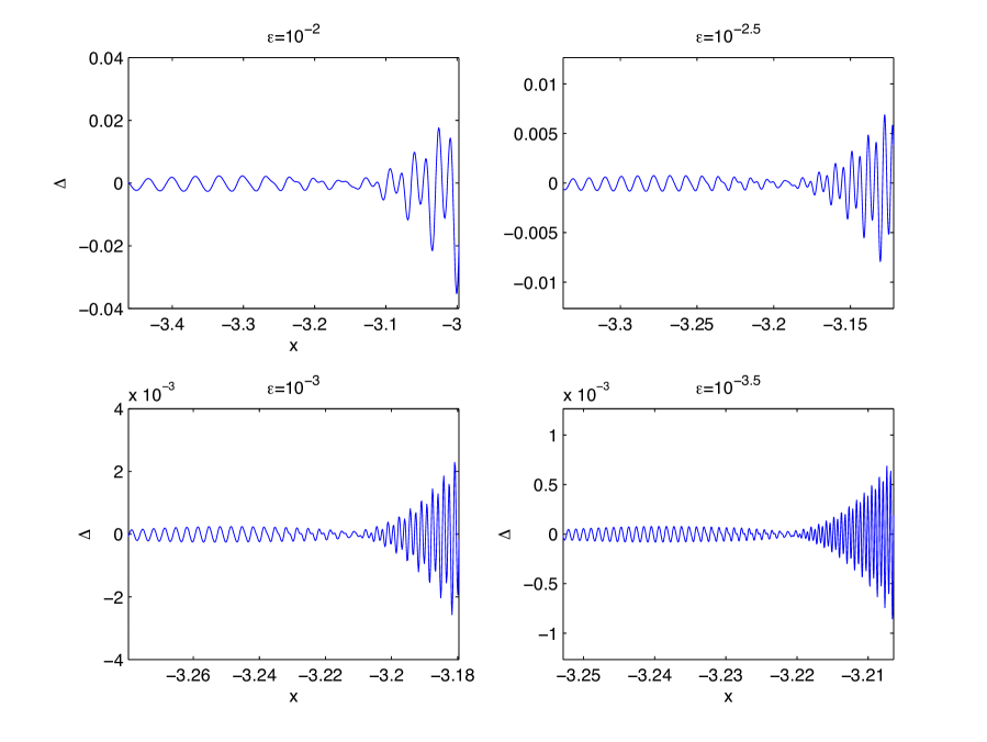
Figure 10. The difference between the numerical solution to the KdV equation for the initial datum $u_{0}=-\mbox{sech}^{2}x$ at $t=0.4$ and the corresponding multiscale solution (2.25) for four values of $\epsilon$. Notice the scaling of the $x$ and $\Delta$ axes with a factor $\epsilon^{2/3}$ and $\epsilon$ respectively to take care of the expected scalings in $x$ and of the shown error next to the leading edge of the Whitham zone.

The difference between KdV solution and the ${\rm P}_{II}$ asymptotics is shown for several values of $\epsilon$ in Fig. 10. It can be seen that the error close to the Whitham edge is almost constant. The scales in $x$ and $\Delta$ are rescaled by a factor $\epsilon^{2/3}$ and $\epsilon$ respectively which is the expected scaling behavior of the zone, where the multiscale solution should be applicable, and of the expected error. It can be seen that with these rescalings the error is of the same order for different values of $\epsilon$. A linear regression analysis for the logarithm of the difference $\Delta$ between KdV and multiscale solution in the interval $[x^{-}-\epsilon^{2/3},x^{-}+\epsilon^{2/3}]$ gives a scaling of the form $\Delta\propto\epsilon^{a}$ with $a=1.00$ with standard deviation $\sigma_{a}=0.004$ and correlation coefficient $r=0.99999$. The result is almost the same in a larger interval, e.g., $[x^{-}-2\epsilon^{2/3},x^{-}+2\epsilon^{2/3}]$ with just a slightly worse correlation. The found scaling is thus as expected of order $\epsilon$.

As can be already seen from Fig. 8, the multiscale solution gives a better asymptotic description of KdV near the leading edge of the Whitham zone than the Hopf and the one-phase KdV solution. This is even more obvious in Fig. 11a where the difference between KdV and the asymptotic solutions is shown.

This suggests to identify the regions where each of the asymptotic solutions gives a better description of KdV than the other. The results of this analysis can be seen in Fig. 12. This matching procedure clearly improves the KdV description near the leading edge. We also show the difference between this matched asymptotic solution and the KdV solution for two values of $\epsilon$. Visibly the zone, where the solutions are matched, decreases with $\epsilon$.

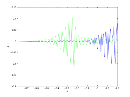
(a)

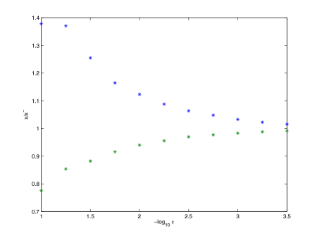
(b)

Figure 11. In Fig. (a) the difference between the numerical solution to the KdV equation for the initial datum $u_{0}=-\mbox{sech}^{2}x$ at $t=0.4$ for $\epsilon=10^{-2}$ and the corresponding ${\rm P}_{II}$ asymptotic solution (2.25) in blue, and the difference between KdV and Hopf and one-phase KdV solution in green. In Fig. (b) the edges of the zone where the ${\rm P}_{II}$ asymptotic solution (2.25) provides a better asymptotic description of KdV than the Hopf or the one-phase KdV solution in dependence of $\epsilon$.

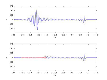
(a)

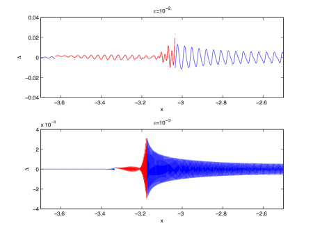
(b)

Figure 12. In the upper part of Fig. (a) one can see the difference between the numerical solution to the KdV equation for the initial datum $u_{0}=-\mbox{sech}^{2}x$ and $\epsilon=10^{-2}$ at $t=0.4$ and the corresponding asymptotic solution in terms of Hopf and one-phase KdV solutions. The lower part shows the same difference, which is replaced close to the leading edge of the Whitham zone by the difference between KdV solution and the ${\rm P}_{II}$ asymptotic solution (2.25) (shown in red where the error is smaller than the one shown above). The figures in (b) show the same situation as in the lower part of (a) for two values of $\epsilon$. Notice the rescaling of the $\Delta$ axis with a factor $\epsilon$, the expected scaling of the error.

There is a certain ambiguity in the precise definition of this matching zone due to the oscillatory character of the solutions. The limits of the matching zone for several values of $\epsilon$ can be seen in Fig. 11b. Due to the lower number of oscillations in the Hopf region, the matching zone extends much further into this region than in the Whitham region. There does not appear to be a clear scaling law for the width of this zone. It can be already seen in Fig. 12 that the error at the matching does not scale with $\epsilon$. In fact we find a scaling close to $\epsilon^{a}$ with $a\sim 2/3$ (in the Whitham zone we find $a=0.63$ and $\sigma_{a}=0.015$ with $r=0.9995$, and in the ${\rm P}_{II}$ zone $a=0.60$ and $\sigma_{a}=0.063$ with $r=0.99$). Thus it is not possible to obtain an error of order $\epsilon$ up to the trailing edge. It is clear that analytic connection formulae between the two asymptotic solutions must be established to obtain an error of order $\epsilon$ in the shown range.

6. Trailing edge

In this section we study numerically for times greater than the critical time the soliton asymptotic formula (2.33) that approximates as $\epsilon\rightarrow 0$ the solution of KdV near the trailing edge of the oscillatory zone. We identify the zone, where this asymptotic formula gives a better description of KdV than the one-phase KdV (2.1) and Hopf (1.4) solutions and study the $\epsilon$-dependence of the errors.

In Fig. 13 we show the KdV solution, the asymptotic solution via Whitham and Hopf and the soliton asymptotics near the trailing edge of the Whitham zone. As before the one-phase KdV solution gives a very good description in the interior of the Whitham zone, whereas the soliton asymptotic formula gives as expected a better description near the trailing edge.

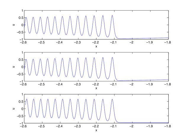
Figure 13. The figure shows in the upper part the numerical solution to the KdV equation for the initial datum $u_{0}=-\mbox{sech}^{2}x$ and $\epsilon=10^{-2}$ at $t=0.4$, in the middle the corresponding asymptotic solution in terms of Hopf and one-phase KdV solution, and in the lower part the multiscale solution (2.33).

In Fig. 14 the KdV and the multiscale solution are shown in one plot for $\epsilon=10^{-2}$. It can be seen that the agreement very close to the boundary of the Whitham zone is once more so good that the difference of the solutions has to be studied. The solution only gives locally an asymptotic description, and the quality of the approximation is not symmetric around the critical point.

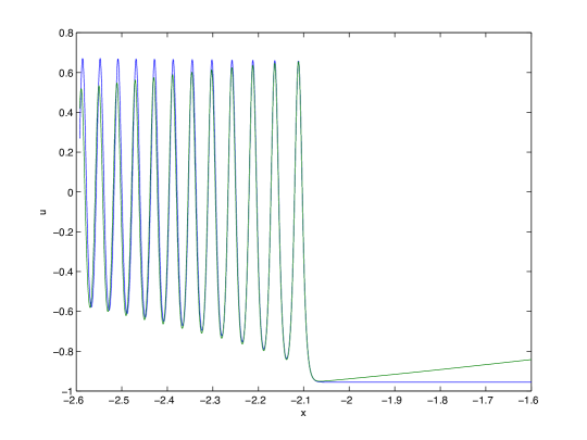
Figure 14. The numerical solution to the KdV equation for the initial datum $u_{0}=-\mbox{sech}^{2}x$ and $\epsilon=10^{-2}$ at $t=0.4$ in blue and the corresponding multiscale solution (2.33) in green.

The difference between KdV solution and the soliton asymptotic solution is shown for several values of $\epsilon$ in Fig. 15. The scales in $x$ and $\Delta$ are both rescaled by a factor $\epsilon$ which is the expected scaling behavior of the zone (numerically $\epsilon$ and $\epsilon\ln\epsilon$ are indistinguishable), where the soliton asymptotic solution should be applicable, and of the expected error. It can be seen that with these rescalings the error is of the same order for different values of $\epsilon$. A linear regression analysis for the logarithm of the difference $\Delta$ between KdV and multiscale solution in the interval $[x^{+}+\epsilon\ln\epsilon,x^{+}-\epsilon\ln\epsilon]$ gives a scaling of the form $\Delta\propto\epsilon^{a}$ with $a=1.07$ with standard deviation $\sigma_{a}=0.056$ and correlation coefficient $r=0.998$. The found scaling is thus compatible with $\epsilon\ln\epsilon$.

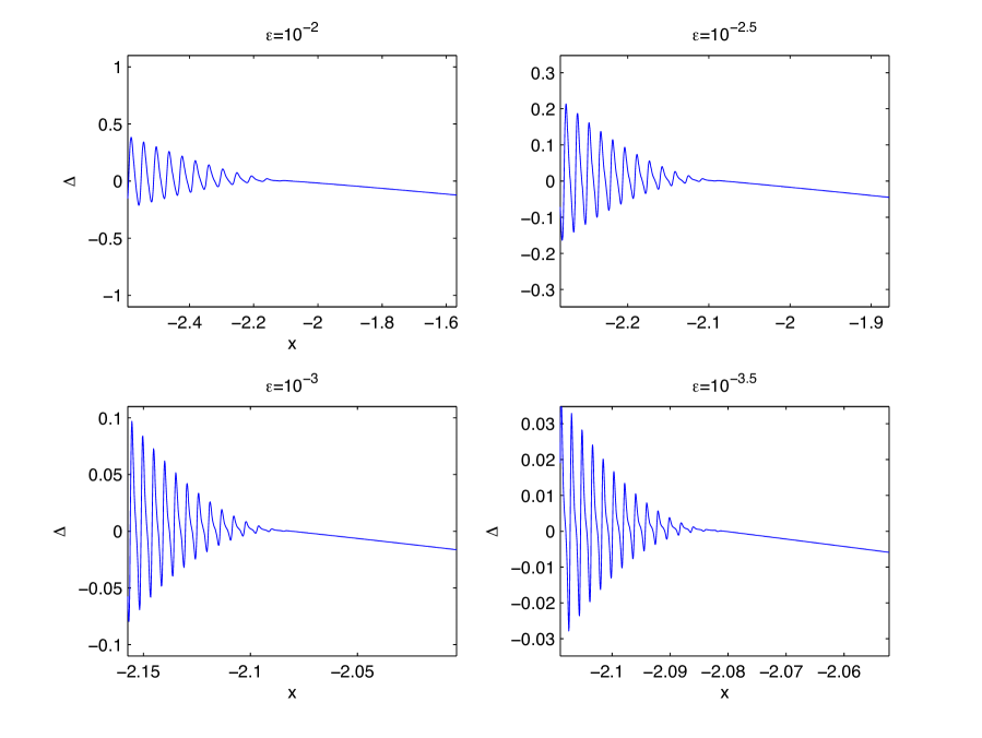
Figure 15. The difference between the numerical solution to the KdV equation for the initial datum $u_{0}=-\mbox{sech}^{2}x$ at $t=0.4$ and the corresponding soliton asymptotic solution (2.33) for four values of $\epsilon$. Note the scaling of the $x$ and $\Delta$ axes with a factor $\epsilon$ to take care of the expected scaling in $x$ and of the shown error next to the trailing edge of the Whitham zone.

It can be seen in Fig. 16a, where the difference between KdV and the asymptotic solutions is shown, that soliton asymptotic solution gives a much a better description of KdV near the trailing edge of the Whitham zone than the Hopf and the one-phase KdV solution.

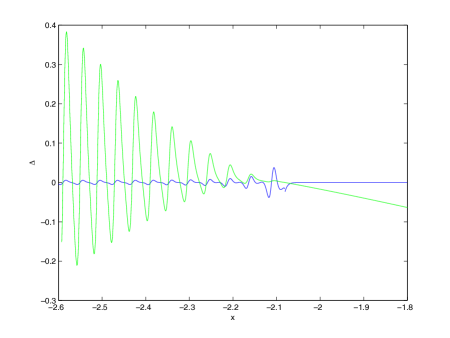
(a)

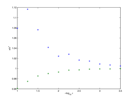
(b)

Figure 16. In Fig. (a), the difference between the numerical solution to the KdV equation for the initial datum $u_{0}=-\mbox{sech}^{2}x$ and $\epsilon=10^{-2}$ at $t=0.4$ and the corresponding soliton asymptotic (2.33) in green, and the difference between KdV and Hopf and one-phase KdV solution in blue. In Fig. (b) the edges of the zone where the soliton asymptotic (2.33) provides a better asymptotic description of KdV than the Hopf or the one-phase KdV solution in dependence of $\epsilon$.

Again we can identify the regions where each of the asymptotic solutions gives a better description of KdV than the other. The results of this analysis can be seen in Fig. 17a. This matching procedure clearly improves the KdV description near the trailing edge. In Fig. 17b we see the difference between this matched asymptotic solution and the KdV solution for two values of $\epsilon$. Visibly the zone, where the solutions are matched, decreases with $\epsilon$.

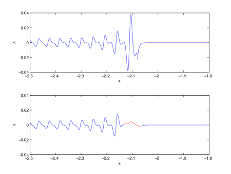
(a)

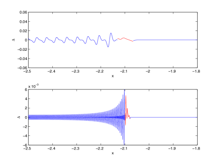
(b)

Figure 17. In the upper part of Fig. (a) one can see the difference between the numerical solution to the KdV equation for the initial datum $u_{0}=-\mbox{sech}^{2}x$ and $\epsilon=10^{-2}$ at $t=0.4$ and the corresponding asymptotic solution in terms of Hopf and one-phase KdV solution. The lower part shows the same difference, which is replaced close to the trailing edge of the Whitham zone by the difference between KdV solution and the soliton asymptotic (2.33) (shown in red where the error is smaller than the one shown above). In Fig. (b) the same situation as in the lower part of (a) is shown for two values of $\epsilon$: $10^{-2},\;10^{-3}$. The $\Delta$-axis is rescaled by a factor $\epsilon$.

Once more there is no precise definition of this matching zone due to the oscillatory character of the solutions. We determine it as the point where the curves of the differences intersect, or where they come closest, before one error dominates the other for all smaller respectively larger values of $x$. The limits of the matching zone for several values of $\epsilon$ can be seen in Fig. 16b. There does not appear to be a clear scaling law for the width of this zone. It can be already seen in Fig. 17b that the error in the matching zone does not scale with $\epsilon$ as close to the boundary of the Whitham zone. In fact we find a scaling close to $\epsilon^{1/2}$ in both cases, but the correlation is not very good. As for the leading edge, it is necessary to establish analytical connection formulae.

7. Point of gradient catastrophe

In this section we study numerically the approximation (2.16) to the solution $u(x,t,\epsilon)$ of KdV as $\epsilon\rightarrow 0$ near the point of gradient catastrophe $(x_{c},t_{c})$ for the solution of the Hopf equation. We identify the zone, where the ${\rm P}_{I}^{2}$ asymptotic formula (2.16) gives a better asymptotic description of KdV than the Hopf or the one-phase KdV solution and study the $\epsilon$-dependence of the errors. We qualitatively study for a time $t>t_{c}$ close to $t_{c}$ how the various multiscale approximations perform.

7.1. Critical time

For the initial datum $u_{0}(x)=-\mbox{sech}^{2}x$ the critical time is $t_{c}=\sqrt{3}/8\sim 0.2165$ and the critical point $x_{c}=-\sqrt{3}/2+\ln((\sqrt{3}-1)/\sqrt{2})\sim-1.5245$. In Fig. 18 we show the KdV solution, the Hopf solution and the multiscale solution near the critical point of the Hopf solution at the critical time. As before the Hopf solution gives a very good description for $|x-x_{c}|\gg 0$, whereas the ${\rm P}_{I}^{2}$ asymptotic solution gives as expected a better description near the critical point. The following figures are always symmetric with respect to $x_{c}$.

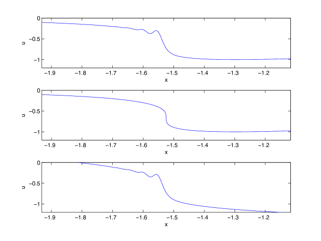
Figure 18. The figure shows in the upper part the numerical solution to the KdV equation for the initial datum $u_{0}=-\mbox{sech}^{2}x$ and $\epsilon=10^{-2}$ at $t=t_{c}$, in the middle the corresponding Hopf solution, and in the lower part the ${\rm P}_{I}^{2}$ asymptotics (2.16).

In Fig. 19 the KdV solution and the ${\rm P}_{I}^{2}$ asymptotic solution are shown in one plot for $\epsilon=10^{-2}$. It can be seen that the agreement very close to the critical point of the Hopf solution is again so good that the difference of the solutions has to be studied. The solution only gives locally an asymptotic description.

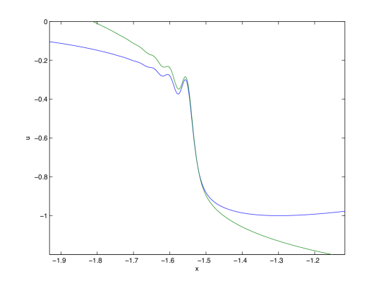
Figure 19. The numerical solution to the KdV equation for the initial datum $u_{0}=-\mbox{sech}^{2}x$ and $\epsilon=10^{-2}$ at $t=t_{c}$ in blue and the corresponding ${\rm P}_{I}^{2}$ asymptotic solution in green.

The difference between KdV solution and ${\rm P}_{I}^{2}$ asymptotic solution is shown for several values of $\epsilon$ in Fig. 20. The scales in $x$ are rescaled by a factor $\epsilon^{6/7}$, and the ones for $\Delta$ by a factor $\epsilon^{5/7}$ respectively which is the expected scaling behavior of the zone, where the ${\rm P}_{I}^{2}$ asymptotic solution should be applicable, and of the expected error. It can be seen that with these rescalings the error is of the same order for different values of $\epsilon$, at least close to the critical point. We also show in this figure the different behaviour of the terms in (2.16) in order $\epsilon^{2/7}$ and order $\epsilon^{4/7}$. The former is not symmetric with respect to the critical point. In fact the approximation is better on the side where the oscillations appear. However if one studies positive initial data as in [31], the oscillations are on the side of the critical point where the approximation in terms of the ${\rm P}_{I}^{2}$ solution is worse.

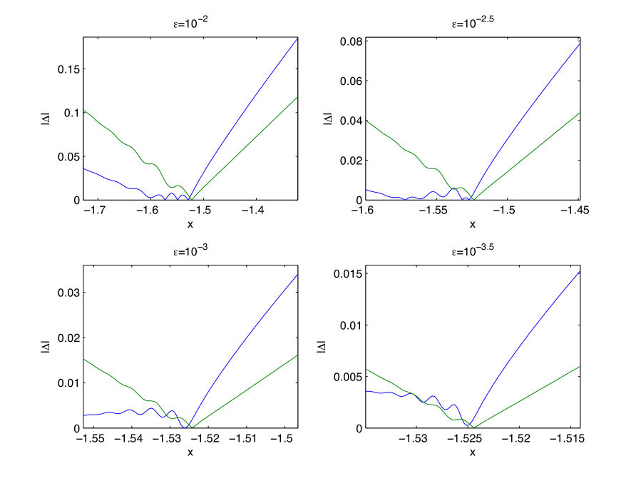
Figure 20. The difference between the numerical solution to the KdV equation for the initial datum $u_{0}=-\mbox{sech}^{2}x$ at $t=t_{c}$ and the corresponding multiscale solution for four values of $\epsilon$, in blue the terms in (2.16) up to order $\epsilon^{2/7}$, in green up to order $\epsilon^{4/7}$. Note the scaling of the $x$ and $\Delta$ axes with a factor $\epsilon^{6/7}$ and $\epsilon^{5/7}$ respectively to take care of the expected scaling in $x$ and of the shown error next to the critical point.

As is clear from Fig. 18, the multiscale solution gives a better asymptotic description of KdV near the critical point than the Hopf. This is even more obvious in Fig. 21a where the difference between KdV and the Hopf solution is shown.

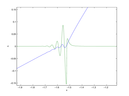
(a)

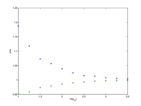
(b)

Figure 21. In Fig. (a) the difference between the numerical solution to the KdV equation for the initial datum $u_{0}=-\mbox{sech}^{2}x$ and $\epsilon=10^{-2}$ at $t=t_{c}$ and the corresponding ${\rm P}_{I}^{2}$ asymptotic solution in blue, and the difference between KdV and Hopf solution in green. In Fig. (b) the edges of the zone where the ${\rm P}_{I}^{2}$ asymptotic solution provides a better asymptotic description of KdV than the Hopf solution in dependence of $\epsilon$.

Again we can identify the regions where each of the asymptotic solutions gives a better description of KdV than the other. The results of this analysis can be seen in Fig. 22a. This matching procedure clearly improves the KdV description near the critical point. In Fig. 22b we see the difference between this matched asymptotic solution and the KdV solution for two values of $\epsilon$. Visibly the zone, where the solutions are matched, decreases with $\epsilon$ (notice the rescaling of the axes with $\epsilon$).

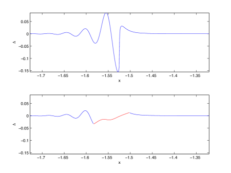
(a)

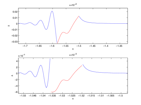
(b)

Figure 22. In the upper part of Fig. (a) one can see the difference between the numerical solution to the KdV equation for the initial datum $u_{0}=-\mbox{sech}^{2}x$ and $\epsilon=10^{-2}$ at $t=t_{c}$ and the corresponding Hopf solution. The lower part shows the same difference, which is replaced close to the critical point by the difference between KdV solution and the ${\rm P}_{I}^{2}$ asymptotic solution (shown in red where the error is smaller than the one shown above). Fig. (b) shows the same situation as the lower figure in (a) for two values of $\epsilon$. The $\Delta$-axis is rescaled by a factor $\epsilon^{5/7}$, the $x$-axis by a factor $\epsilon^{6/7}$.

Once more there is no precise definition of this matching zone due to the oscillatory character of the solutions. We choose it as in the previous sections as given where the curves of the differences intersect, or where they come closest before one error dominates the other. The limits of the matching zone for several values of $\epsilon$ can be seen in Fig. 21b. There does not appear to be a clear scaling law for the width of this zone. A linear regression analysis for the logarithm of the difference $\Delta$ between KdV and multiscale solution in the matching zone gives a scaling of the form $\Delta\propto\epsilon^{a}$ with $a=0.586$ ($4/7\sim 0.5714$) with standard deviation $\sigma_{a}=0.06$ and correlation coefficient $r=0.99$ for the terms up to order $\epsilon^{2/7}$ and with $a=0.62$ ($5/7\sim 0.7143$) with standard deviation $\sigma_{a}=0.09$ and correlation coefficient $r=0.98$ for the terms up to order $\epsilon^{4/7}$. The found scaling is thus compatible with the expected $\epsilon^{4/7}$ and $\epsilon^{5/7}$ respectively. The error in the Hopf zone at the limits of the matching zone are of the same order. As before it would be interesting to study the connection formulae between the Hopf and ${\rm P}_{I}^{2}$ zone.

7.2. Close to the critical time

It is an interesting question to study how the various multiscale approximations perform for a time $t$ greater than the critical time with $t\sim t_{c}$, where all previously studied asymptotic formulae should be applicable. We consider just one value of $\epsilon$ ($\epsilon=10^{-2}$) since the various multiscale expansions use different $\epsilon$-dependent rescalings of the time. We consider the time $t=0.23>t_{c}\sim 0.2165$.

First we study the situation in the vicinity of the leading edge ($x=-1.6051\ldots$). In Fig. 23, the KdV solution can be seen in this case as well as the asymptotic solution in terms of Hopf and one-phase KdV solution, the multiscale solution (2.25) near the leading edge and the multiscale solution (2.16) close to the critical point.

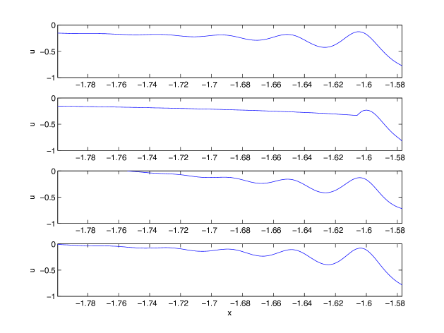
Figure 23. The figure shows from top to bottom the numerical solution to the KdV equation for the initial datum $u_{0}=-\mbox{sech}^{2}x$ and $\epsilon=10^{-2}$ at $t=0.23>t_{c}$, the asymptotic solution in terms of Hopf and one-phase KdV solution, the multiscale solution (2.25), and the multiscale solution (2.16).

In Fig. 24 the same solutions can be seen in one figure.

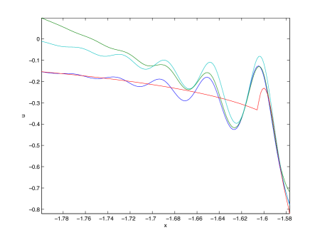
(a)

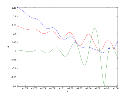
(b)

Figure 24. Fig. (a) shows the numerical solution to the KdV equation for the initial datum $u_{0}=-\mbox{sech}^{2}x$ and $\epsilon=10^{-2}$ at $t=0.23>t_{c}$ in blue, the asymptotic solution in terms of Hopf and one-phase KdV solution in red, the multiscale solution (2.25) in cyan, and the multiscale solution (2.16) in green. Fig. (b) shows the difference between the asymptotic solution in terms of Hopf and one-phase KdV solution and the numerical solution to the KdV equation in green, between the ${\rm P}_{II}$ asymptotic solution (2.25) and KdV in red, and the ${\rm P}_{I}^{2}$ asymptotic solution (2.16) and KdV in blue.

It can be seen already from these figures or from the plot of the differences between the asymptotic solutions and the KdV solution in Fig. 24b that the asymptotic solution in terms of Hopf and one-phase KdV solution performs worst close to the leading edge, and that the multiscale solution (2.16) in terms of the ${\rm P}_{I}^{2}$ transcendent is most satisfactory. The multiscale solution (2.25) is only very close to the leading better than the ${\rm P}_{I}^{2}$ asymptotics. It captures qualitatively the oscillations in the Hopf region, but is not oscillating around the Hopf solution as KdV. As can be seen from (2.25) the reason for this is that the amplitude of this solution is divided by $u-v$ which tends to 0 at the critical point. The ${\rm P}_{I}^{2}$ asymptotics also quickly becomes out of phase in the Hopf region. Thus to obtain a satisfactory description of the small dispersion limit of KdV close to the critical point, one has to study connection formulae between the various asymptotic solutions.

The situation near the trailing edge ($x=-1.5757\ldots$) is similar. In Fig. 25, the KdV solution can be seen in this case as well as the asymptotic solution in terms of Hopf and one-phase KdV solution, the multiscale solution (2.33) near the leading edge and the multiscale solution (2.16) close to the critical point.

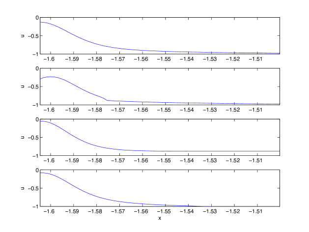
Figure 25. The figure shows from top to bottom the numerical solution to the KdV equation for the initial datum $u_{0}=-\mbox{sech}^{2}x$ and $\epsilon=10^{-2}$ at $t=0.23>t_{c}$, the asymptotic solution in terms of Hopf and one-phase KdV solution, the soliton asymptotic solution (2.33), and the ${\rm P}_{I}^{2}$ asymptotic solution (2.16).

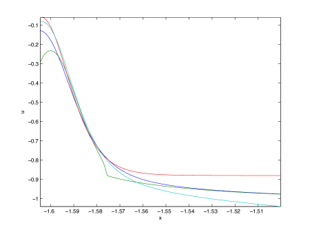
(a)

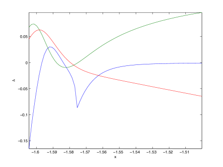
(b)

Figure 26. Fig. (a) shows the numerical solution to the KdV equation for the initial datum $u_{0}=-\mbox{sech}^{2}x$ and $\epsilon=10^{-2}$ at $t=0.23>t_{c}$ in blue, the asymptotic solution in terms of Hopf and one-phase KdV solution in green, the multiscale solution (2.33) in red, and the multiscale solution (2.16) in cyan. Fig. (b) shows the difference between the asymptotic solution in terms of Hopf and one-phase KdV solution and the numerical solution to the KdV in blue, between the soliton asymptotic solution (2.33) and KdV in green, and the ${\rm P}_{I}^{2}$ asymptotic solution (2.16) and KdV in red.

In Fig. 26 the same solutions can be seen in one figure. These figures as well as the plot of the differences between the asymptotic solutions and the KdV solution in Fig. 26b show that the asymptotic solution in terms of Hopf and one-phase KdV solution performs worst close to the trailing edge, and that the ${\rm P}_{I}^{2}$ asymptotic solution (2.16) performs best. The soliton asymptotic solution (2.25) is better than the ${\rm P}_{I}^{2}$ asymptotics only very close to the trailing edge. The ${\rm P}_{I}^{2}$ asymptotics also quickly becomes unsatisfactory in the Hopf region. Thus to obtain a better description of the small dispersion limit of KdV close to the critical point, one has to study connection formulae between the various asymptotic solutions.

8. Outlook

The numerical results of the previous sections have shown that the proposed asymptotic descriptions lead in fact to an error of order $\epsilon$ in various regions of the $x,t$-plane where the respective formulae are supposed to hold. However the asymptotic description at the trailing edge of the oscillatory zone and the point of gradient catastrophe are characterized by errors of higher order. In order to obtain a complete analytic asymptotic description in the $(x,t)$ plane, analytic connection formulae have to be established between the various asymptotic formulae. For example, despite the asymptotic formulas (2.1) and (2.25) having an error of order $\epsilon$, the numerical results show that there is still a region near the leading edge at the boundary of the Whitham zone where the error is bigger. This means that a connection formula between the elliptic expansion (2.1) and the expansion (2.25) (where the terms of order $\epsilon^{\frac{2}{3}}$ have been dropped), is needed.

In [13] Claeys has derived connection formula for the ${\rm P}_{I}^{2}$ solution $U(X,T)$ of (2.11) in different regions of the $(X,T)$ plane. Using these relations, one can derive in a non rigorous way the corresponding connection formulas for the asymptotic solution of the KdV equation near the point of gradient catastrophe. Indeed the ${\rm P}_{\rm I}^{2}$ solution $U(X,T)$ describes a singular transition between a region of simple algebraic asymptotics and a region of more complicated oscillatory asymptotics involving the Jacobi elliptic $\theta$-function. One may thus expect that $U(X,T)$ itself also exhibits different types of asymptotics. Indeed the following result holds [13]:

• $X\rightarrow\pm\infty$ and $T\rightarrow-\infty$ or $T\rightarrow+\infty$ in such a way $S=\dfrac{X}{T^{\frac{3}{2}}}$ remains bounded away from the interval $[-12\sqrt{3},\,\dfrac{4\sqrt{15}}{9}]$, then $U(X,T)$ has an algebraic asymptotics;

• if $-12\sqrt{3}<S<\dfrac{4\sqrt{15}}{9}$, then $U(X,T)$ has an elliptic asymptotics;

• for $S\rightarrow-12\sqrt{3}$, $U(X,T)$ has a ${\rm P}_{II}$ asymptotics;

• for $S\rightarrow\dfrac{4\sqrt{15}}{9}$, $U(X,T)$ has a soliton-like asymptotics.

Substituting the algebraic asymptotic [13] of the ${\rm P}_{\rm I}^{2}$ solution into the asymptotic expansion (2.16), one obtains in a non rigorous way the connection formula between the Hopf asymptotic solution (1.4) and (2.16). More precisely in the limit when

$$X=\dfrac{x-x_{c}-6u_{c}(t-t_{c})}{(k)^{1/7}\epsilon^{\frac{6}{7}}},\quad T=\dfrac{t-t_{c}}{(k)^{3/7}\epsilon^{\frac{4}{7}}}$$

goes to infinity in such a way that $s=\dfrac{X}{T^{\frac{3}{2}}}=\sqrt{k}\dfrac{x-x_{c}-6u_{c}(t-t_{c})}{(t-t_{c})^{\frac{3}{2}}}$ is outside the interval $(-12\sqrt{3},\dfrac{4\sqrt{15}}{9})$, or $T\rightarrow-\infty$ then the solution of the KdV equation is approximated by

$$u(x,t,\epsilon)=u_{c}+z(s)\left(\dfrac{t-t_{c}}{\sqrt{k}}\right)^{\frac{1}{2}}+O\left(\dfrac{\epsilon^{\frac{4}{7}}}{t-t_{c}}\right).$$

where $z(s)$ solves the equation $s=6z-z^{3}$. The second term on the right hand side of the above expression coincides with the solution of the Hopf equation with initial data $f_{L}(u)=-ku^{3}$.

8.1. ${\rm P}_{I}^{2}$ asymptotics and elliptic asymptotics

The asymptotic expansions (2.1) and (2.16) have a connection region that follows from substituting into (2.16) the elliptic asymptotics for the ${\rm P}_{I}^{2}$ solution obtained in [13]. In the limit when

$$X=\dfrac{x-x_{c}-6u_{c}(t-t_{c})}{(k)^{1/7}\epsilon^{\frac{6}{7}}},\quad T=\dfrac{t-t_{c}}{(k)^{3/7}\epsilon^{\frac{4}{7}}}$$

goes to infinity in such a way that $-12\sqrt{3}<s=\dfrac{X}{T^{\frac{3}{2}}}=\sqrt{k}\dfrac{x-x_{c}-6u_{c}(t-t_{c})}{(t-t_{c})^{\frac{3}{2}}}<\dfrac{4\sqrt{15}}{9}$, then the solution of the KdV equation is approximated by

(8.1) $$u(x,t,\epsilon)=u_{c}+\dfrac{\sqrt{t-t_{c}}}{\sqrt{k}}\left(b_{1}+b_{2}+b_{3}+2\alpha+\dfrac{b_{1}-b_{3}}{2K^{2}(s)}(\log\vartheta)^{\prime\prime}(\tilde{\Omega}(s,t);\mathcal{T})\right)+O\left(\dfrac{\epsilon^{\frac{4}{7}}}{\sqrt{t-t_{c}}}\right),$$

where $\alpha$, $s$ and $\mathcal{T}$ are defined in (2.3) (with the substitution $\beta_{i}\rightarrow b_{i}$) and the argument of the Jacobi elliptic function $\vartheta$ is given by

(8.2) $$\tilde{\Omega}=\dfrac{(t-t_{c})^{\frac{7}{4}}\sqrt{b_{1}-b_{3}}}{2\epsilon K(s)k^{\frac{3}{4}}}(s-2(b_{1}+b_{2}+b_{3})-q).$$

Here the quantities $b_{i}=b_{i}(s)$, with $b_{1}(s)>b_{2}(s)>b_{3}(s)$, describe the Gurevich-Pitaevski [43] self-similar solution of the Whitham equations (2.7) with cubic initial data, namely the function $q=q(b_{1},b_{2},b_{3})$ in (2.4) is such that $q(b,b,b)=b^{3}$ and the hodograph transform (2.8) takes the equivalent form [42]

(8.3) $$\begin{split}&6=-\sum_{i=1}^{3}\dfrac{\partial}{\partial b_{i}}q=\dfrac{1}{5}\left[(b_{1}+b_{2}+b_{3})^{2}+2(b_{1}^{2}+b_{2}^{2}+b_{3}^{2})\right]\\ &s=\sum_{i=1}^{3}(2b_{i}-b_{1}+b_{2}+b_{3})\dfrac{\partial}{\partial b_{i}}q+q=\dfrac{2}{15}\left[(b_{1}+b_{2}+b_{3})^{3}-4(b_{1}^{3}+b_{2}^{3}+b_{3}^{3})\right]\\ &\int_{b_{3}}^{b_{2}}\sqrt{(\xi-b_{1})(\xi-b_{2})(\xi-b_{3})}(\xi+\dfrac{1}{2}(b_{1}+b_{2}+b_{3}))d\xi=0.\end{split}$$

The asymptotic expansion (8.1) should give the connection formula near the point of gradient catastrophe $(x_{c},t_{c})$ between the one-phase KdV asymptotics (2.1) and ${\rm P}_{I}^{2}$ asymptotics (2.16). It is straightforward to check that formula (2.1) reduces to (8.1) by expanding the initial data for the Whitham equations at the point of gradient catastrophe and keeping the first order correction (cubic term). Namely, if $\beta_{i}$, $i=1,2,3$ is the solution of the Whitham equation with the initial data (1.1) and $b_{i}$ is the self-similar solution defined in (8.3), then

$$\beta_{i}(x,t)=u_{c}+\sqrt{\dfrac{t-t_{c}}{k}}b_{i}(s)+O(t-t_{c}).$$

With this formula (8.1) can be recovered from (2.1) by the above substitution.The error in this limit is of order $t-t_{c}$. The connection formula (8.1) has already appeared in [38].

8.2. Connection between ${\rm P}_{I}^{2}$ asymptotic and ${\rm P}_{II}$ asymptotic or soliton asymptotic

When $S=-12\sqrt{3}$ the ${\rm P}_{I}^{2}$ solution has an asymptotic expansion that is provided by oscillations whose envelope is given by the Hasting McLeod solution of the Painlevé II equation [13]. Plugging this expansion into (2.16), one obtains in a non rigorous way the connection formula between (2.16) and the ${\rm P}_{II}$ asymptotic solution (2.25), where the terms of order $\epsilon^{\frac{2}{3}}$ have been dropped. Introducing the variable

$$\xi=-\dfrac{X+12\sqrt{3}T^{\frac{3}{2}}}{c_{0}c_{1}T^{\frac{1}{3}}}=-\dfrac{x-x_{c}-6u_{c}(t-t_{c})+12\sqrt{3}k^{-\frac{1}{2}}(t-t_{c})^{\frac{3}{2}}}{\epsilon^{\frac{2}{3}}c_{0}(t-t_{c})^{\frac{1}{3}}},\quad c_{0}=\dfrac{2^{\frac{7}{6}}3^{\frac{1}{12}}}{5^{\frac{1}{6}}},\;\;c_{1}=\sqrt{\dfrac{5\sqrt{3}}{2}}$$

in the ${\rm P}_{I}^{2}$ asymptotic solution (2.16) and letting $T\rightarrow+\infty$ in such a way that $XT^{-\frac{3}{2}}=12\sqrt{3}$ one obtains from [13]

(8.4) $$u(x,t,\epsilon)=u_{c}+2\sqrt{3}\sqrt{\dfrac{t-t_{c}}{k}}-\dfrac{q(\xi)\left(\dfrac{\epsilon}{k}\right)^{\frac{1}{3}}}{c_{0}\left(\dfrac{t-t_{c}}{k}\right)^{\frac{1}{12}}}\cos\left(\dfrac{(t-t_{c})^{\frac{7}{4}}}{\epsilon k^{\frac{3}{4}}}\omega\right)+O\left(\left(\dfrac{\epsilon^{\frac{4}{7}}}{t-t_{c}}\right)^{\frac{2}{3}}\right)$$

where $q(\xi)$ is the Hasting-McLeod solution of Painlevé II, and the phase $\omega$ is given by

$$\omega=\dfrac{88}{7}c_{1}^{3}+2c_{1}^{2}c_{0}\xi\left(\dfrac{t-t_{c}}{k^{\frac{3}{7}}\epsilon^{\frac{4}{7}}}\right)^{-\frac{7}{6}}.$$

This expansion coincides with (2.25) when the initial data at time $t=t_{c}$ is approximated by the cubic initial data $f_{L}(u)=-k(u-u_{c})^{3}+O(u-u_{c})^{4}$ with $k$ defined in (2.15). Indeed in this case the solution of system (2.20)-(2.22) takes the form

$$\begin{split}&x^{-}(t)-x_{c}-6u_{c}(t-t_{c})=12\sqrt{3}\dfrac{(t-t_{c})^{\frac{3}{2}}}{\sqrt{k}}+O((t-t_{c})^{\frac{5}{2}}),\\ &u(t)-u_{c}=2\sqrt{3}\sqrt{\dfrac{t-t_{c}}{k}}+O(t-t_{c}),\quad v(t)-u_{c}=-\dfrac{\sqrt{3}}{2}\sqrt{\dfrac{t-t_{c}}{k}}+O(t-t_{c}).\end{split}$$

Then plugging the above expressions of $x^{-}(t)$, $u(t)$ and $v(t)$ into (2.25) one arrives at (8.4) (with a different error term though).

The ${\rm P}_{I}^{2}$ solution has a connection region with the soliton asymptotics (2.33) when $S=\dfrac{4}{9}\sqrt{15}$ [13]. Substituting the corresponding connection formula in [13] into (2.16) one obtains in a non rigorous way the connection formula for the asymptotic expansions (2.16) and (2.33). Indeed introducing the variable

$$\xi=-\dfrac{8}{7}c_{0}^{2}\dfrac{X-\dfrac{4}{9}\sqrt{15}T^{\frac{3}{2}}}{T^{-\frac{1}{4}}\log T}=-\dfrac{8}{7}c_{0}^{2}\dfrac{x-x_{c}-6u_{c}(t-t_{c})-\dfrac{4}{9}\sqrt{15k}(t-t_{c})^{\frac{3}{2}}}{\epsilon(t-t_{c})^{-\frac{1}{4}}\log\left(\dfrac{t-t_{c}}{\epsilon^{\frac{4}{7}}k^{\frac{3}{7}}}\right)},\quad c_{0}=\sqrt{\dfrac{7}{6}}(15)^{\frac{1}{4}},$$

where $X$ and $T$ are defined as in (2.14), and letting $T\rightarrow+\infty$ in such a way that $XT^{-\frac{3}{2}}=\dfrac{4}{9}\sqrt{15}$ then

(8.5) $$\begin{split}u(x,t,\epsilon)&=u_{c}-2\sqrt{\dfrac{5}{3}}\left(\dfrac{t-t_{c}}{k}\right)^{\frac{1}{2}}+2c_{0}^{2}\left(\dfrac{t-t_{c}}{k}\right)^{\frac{1}{2}}\sum_{j}{\rm sech}^{2}X_{j}+\\ &O\left(\left(\dfrac{t-t_{c}}{\epsilon^{\frac{4}{7}}}\right)^{-\frac{5}{4}}\log^{2}\left(\dfrac{t-t_{c}}{\epsilon^{\frac{4}{7}}}\right)\right)\end{split}$$

where

(8.6) $$\begin{split}&X_{j}=-\frac{7}{8}(\frac{1}{2}-\xi+j)\ln T-\ln(\sqrt{2\pi}h_{j})-(j+\frac{1}{2})\log\left(\dfrac{16c_{0}^{\frac{5}{2}}}{(15)^{\frac{1}{4}}}\right),\\ &h_{j}=\dfrac{2^{\frac{j}{2}}}{\pi^{\frac{1}{4}}\sqrt{j!}}.\end{split}$$

This connection formula coincides with (2.33) when the initial data at $t=t_{c}$ is approximated by the cubic initial data $f_{L}(u)=-k(u-u_{c})^{3}+O(u-u_{c})^{4}$ where $k$ is defined in (2.15). In this case the solution of the system of equation (2.29)- (2.31) takes the form $x^{+}(t)-x_{c}-6u_{c}(t-t_{c})=\dfrac{4\sqrt{15}}{9\sqrt{k}}(t-t_{c})^{\frac{3}{2}}+O((t-t_{c})^{\frac{5}{2}})$, $u(t)-u_{c}=-\dfrac{2}{3}\sqrt{15}\sqrt{\dfrac{t-t_{c}}{k}}+O(t-t_{c})$ and $v(t)-u_{c}=\dfrac{1}{2}\sqrt{15}\sqrt{\dfrac{t-t_{c}}{k}}+O(t-t_{c})$. Plugging the above expressions of $x^{+}(t)$, $u(t)$ and $v(t)$ into (2.33) one obtains the connection formula (8.5).

The rigorous derivation of the above connection formulas and their numerical implementation will be investigated in a subsequent publication.

References

- [1] S. Abenda, T. Grava, C. Klein, Numerical Solution of the Small Dispersion Limit of the Camassa-Holm and Whitham Equations and Multiscale Expansions, SIAM J. Appl. Math. 70, Issue 8, . 2797-2821 (2010).
- [2] J.-P. Berrut, L.N. Trefethen, Barycentric Lagrange Interpolation, SIAM REVIEW 46, No. 3, pp. 501 517 (2004).
- [3] M. Bertola, A. Tovbis, Universality for the focusing nonlinear Schroedinger equation at the gradient catastrophe point: Rational breathers and poles of the tritronquée solution to Painlevé I. Preprint http://xxx.lanl.gov/pdf/1004.1828
- [4] M. Bertola, A. Tovbis, Universality in the profile of the semiclassical limit solutions to the focusing nonlinear Schrödinger equation at the first breaking curve. Int. Math. Res. Not. IMRN 11 (2010), 2119 2167.
- [5] Bertola, M.; Lee, S.Y. First Colonization of a Spectral Outpost in Random Matrix Theory, Constr. Approx. 31 (2010), no. 2, 231 257.
- [6] P. Bleher and A. Its, Double scaling limit in the random matrix model: the Riemann-Hilbert approach, Comm. Pure Appl. Math. 56 (2003), 433-516.
- [7] F. Bornemann, T.A. Driscoll and L.N. Trefethen, ‘The Chebop System for Automatic Solution of Differential Equations’. BIT 48, pp. 701-723 (2008)
- [8] F. Bornemann, ‘On the Numerical Evaluation of Fredholm Determinants’, Math. Comp. 79: 871-915 (2010)
- [9] M.J. Bowick and E. Brézin, Universal scaling of the tail of the density of eigenvalues in random matrix models, Phys. Lett. B 268 (1991), no. 1, 21-28.
- [10] E. Brézin, E. Marinari, and G. Parisi, A nonperturbative ambiguity free solution of a string model. Phys. Lett. B 242 (1990), no. 1, 35–38.
- [11] R.J. Buckingham, P.D. Miller, The sine-Gordon equation in the semiclassical limit: critical behavior near a separatrix. Preprint http://xxx.lanl.gov/pdf/1106.5716.
- [12] J. Certaine, Mathematical Methods for digital Computers (Wiley, 1960)
- [13] T. Claeys, Asymptotics for a special solution to the second member of the Painlev I hierarchy. J. Phys. A 43 (2010), no. 43, 434012, 18 pp.
- [14] T. Claeys, Birth of a cut in unitary random matrix ensembles. Int. Math. Res. Not. 2008 (2008), no. 6, Art. ID rnm166.
- [15] T. Claeys and T. Grava, Universality of the break-up profile for the KdV equation in the small dispersion limit using the Riemann-Hilbert approach, Comm. Math. Phys., 286 (2009), 979–1009.
- [16] T. Claeys, T. Grava, Painlevé II asymptotics near the leading edge of the oscillatory zone for the Korteweg-de Vries equation in the small-dispersion limit. Comm. Pure Appl. Math. 63 (2010), no. 2, 203 232.
- [17] T. Claeys, T. Grava, Solitonic asymptotics for the Korteweg-de Vries equation in the small dispersion limit. SIAM J. Math. Anal. 42 (2010), no. 5, 2132 2154.
- [18] T. Claeys, T. Grava, The KdV hierarchy: universality and a Painleve transcendent. Preprint http://xxx.lanl.gov/pdf/1101.2602.
- [19] T. Claeys and A.B.J. Kuijlaars, Universality of the double scaling limit in random matrix models, Comm. Pure Appl. Math. 59 (2006), no. 11, 1573-1603.
- [20] T. Claeys, A.B.J. Kuijlaars, and M. Vanlessen, Multi-critical unitary random matrix ensembles and the general Painlevé II equation, Ann. Math. 167 (2008), 601-642.
- [21] T. Claeys and M. Vanlessen, The existence of a real pole-free solution of the fourth order analogue of the Painleve I equation, Nonlinearity 20 (2007), 1163–1184.
- [22] T. Claeys and M. Vanlessen, Universality of a double scaling limit near singular edge points in random matrix models, Comm. Math. Phys. 273 (2007), 499–532.
- [23] J. Colliander, M. Keel, G. Staffilani, H. Takaoka, T. Tao, Global well-posedness for KdV in Sobolev Spaces of negative index Electronic Journal of Differential Equations, Vol 2001 No. 26, (2001), 1 7. ISSN: 1072-6691. URL: http://ejde.math.swt.edu or http://ejde.math.unt.edu
- [24] S.M. Cox and P.C. Matthews, Exponential Time Differencing for stiff Systems, J. Comp. Phys., 176, 430–455 (2002)
- [25] P. Deift, Orthogonal Polynomials and Random Matrices: A Riemann-Hilbert Approach, Courant Lecture Notes 3, New York University 1999.
- [26] P. Deift, S. Venakides, and X. Zhou, New result in small dispersion KdV by an extension of the steepest descent method for Riemann-Hilbert problems. Internat. Math. Res. Notices 6 (1997), 285–299.
- [27] P. Deift, T. Kriecherbauer, K.T-R McLaughlin, S. Venakides, X. Zhou, Strong asymptotics of orthogonal polynomials with respect to exponential weights, Comm. Pure Appl. Math. 52 (1999), 1491-1552.
- [28] B. Dubrovin, On Hamiltonian perturbations of hyperbolic systems of conservation laws, II: universality of critical behaviour, Comm. Math. Phys. 267 (2006), no. 1, 117-139.
- [29] B. Dubrovin, On universality of critical behaviour in Hamiltonian PDEs, arXiv:0804.3790, Amer. Math. Soc. Transl., vol. 224 (2008) 59-109.
- [30] B. Dubrovin, T. Grava, C. Klein, On universality of critical behaviour in the focusing nonlinear Schrödinger equation, elliptic umbilic catastrophe and the tritronquée solution to the Painlevé-I equation, J. Nonl. Sci. Vol. 19(1), 57-94 (2009).
- [31] B. Dubrovin, T. Grava, C. Klein, Numerical Study of breakup in generalized Korteweg-de Vries and Kawahara equations, SIAM J. Appl. Math., Vol 71, 983-1008 (2011).
- [32] M. Duits and A.B.J. Kuijlaars, Painlevé I asymptotics for orthogonal polynomials with respect to a varying quartic weight, Nonlinearity 19 (2006), no. 10, 2211-2245.
- [33] B. Eynard, Universal distribution of random matrix eigenvalues near the ”birth of a cut” transition, J. Stat. Mech. 7 (2006), P07005.
- [34] A.S. Fokas, A.R. Its, and A.V. Kitaev. The isomonodromy approach to matrix models in 2D quantum gravity, Comm. Math. Phys. 147 (1992), 395-430.
- [35] A.S. Fokas, A.R. Its, A.A. Kapaev, and V.Yu. Novokshenov, “ Painlevé transcendents: the Riemann-Hilbert approach”, AMS Mathematical Surveys and Monographs 128 (2006).
- [36] B. Fornberg, A practical guide to pseudospectral methods, (Cambridge University Press, Cambridge 1996)
- [37] B. Fornberg and J.A.C. Weideman, ‘A numerical methodology for the Painlevé equations’, J. Comp. Phys. 230 (2011) 5957 5973.
- [38] R. Garifullin, B. Suleimanov, N. Tarkhanov, Phase shift in the Whitham zone for the Gurevich-Pitaevskii special solution of the Korteweg-de Vries equation. Phys. Lett. A 374 (2010), no. 13-14, 1420 1424,
- [39] T. Grava and C. Klein, Numerical solution of the small dispersion limit of Korteweg de Vries and Whitham equations, Comm. Pure Appl. Math. 60 (2007), no. 11, 1623-1664.
- [40] T. Grava and C. Klein, Numerical study of a multiscale expansion of the Korteweg-de Vries equation and Painlevé II equation, Proc. R. Soc. Lond. Ser. A Math. Phys. Eng. Sci. 464 (2008), no. 2091, 733-757. .
- [41] T. Grava, C. Klein, Numerical study of a multiscale expansion of KdV and Camassa-Holm equation, in Integrable Systems and Random Matrices, ed. by J. Baik, T. Kriecherbauer, L.-C. Li, K.D.T-R. McLaughlin and C. Tomei, Contemp. Math. Vol. 458, 81-99 (2008).
- [42] T. Grava, F.-R. Tian, The generation, propagation, and extinction of multiphases in the KdV zero-dispersion limit. Comm. Pure Appl. Math. 55 (2002), no. 12, 1569–1639.
- [43] A. G. Gurevich, L. P. Pitaevskii, Non stationary structure of a collisionless shock waves, JEPT Letters 17 (1973), 193–195.
- [44] S.P. Hastings and J.B. McLeod, A boundary value problem associated with the second Painlevé transcendent and the Korteweg-de Vries equation, Arch. Rational Mech. Anal. 73 (1980), 31-51.
- [45] M. Hochbruck, A. Ostermann, Exponential Runge-Kutta Methods for semilinear parabolic Problems, SIAM J. Numer. Anal., 43 (2005), 1069 1090.
- [46] M. Hochbruck, A. Ostermann, Exponential Integrators, Acta Numerica, 19 (2010), 209 286.
- [47] S. Kamvissis, K.D.T-R. McLaughlin, P.D. Miller, Semiclassical soliton ensembles for the focusing nonlinear Schrödinger equation, Ann. Math. Studies 154, Princeton Univ. Press, Princeton (2003).
- [48] C. Klein, Fourth-Order Time-Stepping for low Dispersion Korteweg-de Vries and nonlinear Schrödinger Equation, Electronic Transactions on Numerical Analysis, 39 (2008), 116 13
- [49] J. C. Lagarias, J. A. Reeds, M. H. Wright, P. E. Wright, Convergence Properties of the Nelder-Mead Simplex Method in Low Dimensions, SIAM Journal of Optimization 9 (1998), no. 1, 112-147.
- [50] P.D. Lax and C.D. Levermore, The small dispersion limit of the Korteweg de Vries equation, I,II,III, Comm. Pure Appl. Math. 36 (1983), 253-290, 571-593, 809-830.
- [51] D. Masoero, A. Raimondo, Semiclassical limit for generalized KdV equations before the gradient catastrophe. Preprint http://xxx.lanl.gov/pdf/1107.0461
- [52] M.Y. Mo, The Riemann-Hilbert approach to double scaling limit of random matrix eigenvalues near the “birth of a cut” transition. Int. Math. Res. Not. 2008 (2008), no. 13, Art. ID rnn042.
- [53] S. Olver, Numerical solution of Riemann Hilbert problems: Painlev II, Found. Comput. Maths, 11: 153 179 (2011).
- [54] B. I. Suleimanov, Solution of the Korteweg-de Vries equation which arises near the breaking point in problems with a slight dispersion. JETP Lett. 58 (1993), no. 11, 849 854;
- [55] F.-R. Tian, Oscillations of the zero dispersion limit of the Korteweg-de Vries equation, Comm. Pure Appl. Math. 46 (1993), 1093-1129.
- [56] Fei-Ran Tian, The initial value problem for the Whitham averaged system. Comm. Math. Phys. 166 (1994), no. 1, 79–115.
- [57] L. N. Trefethen, Spectral Methods in MATLAB, SIAM, Philadelphia, PA, 2000.
- [58] S. P. Tsarev, Poisson brackets and one–dimensional Hamiltonian systems of hydrodynamic type., Dokl. Akad. Nauk. SSSR 282 (1985), 534–537.
- [59] S. Venakides, The Korteweg de Vries equations with small dispersion: higher order Lax-Levermore theory. Comm. Pure Appl. Math. 43 (1990), 335-361.
- [60] G.B. Whitham, “ Linear and nonlinear waves”, J.Wiley, New York, 1974.